Consequences of the local spin self-energy approximation on the heavy Fermion quantum phase transition

Abstract

We show, using the periodic Anderson model, that the local spin self-energy approximation, as implemented in the extended dynamical mean field theory (EDMFT), results in a first order phase transition which persists to $T=0$. Around the transition, there is a finite coexistence region of the paramagnetic and antiferromagnetic (AFM) phases. The region is bounded by two critical transition lines which differ by an electron-hole bubble at the AFM ordering wave vector.

I Introduction.

Competing Kondo and RKKY interactions in Heavy Fermion materials induce a quantum phase transition doniach (1, 2) near which various deviations from the Landau-Fermi liquid behavior are observed experimentally stewart (3). Among the well-studied heavy Fermion compounds is $CeCu_{6-x}Au_{x}$ lohneysen (4) on which neutron scattering and magnetometry experiments showed schroder (5) that, in the quantum critical region, the spin susceptibilities, both the homogeneous one and that at the antiferromagnetic (AFM) ordering wave vector, followed,

$$\chi^{-1}(\vec{q},T)=\left[T^{\alpha}+\theta^{\alpha}(\vec{q})\right]/C$$ (1)

with $T$ the temperature, $\theta(\vec{q})$ a momentum dependent function which is a measure of the distance from the critical wave-vector, and $C$ the Curie constant. In the experiments it was found the exponent $\alpha\sim 0.75$, unlike $\alpha=1$ in the standard Curie-Weiss law. This same behavior was found, within experimental error, to be followed by the neutron scattering data taken at the other wave vectors. The disentanglement of the temperature and momentum dependences in the inverse spin susceptibilities led to the suggestion si0 (6) that the self-energy of the spin-spin interaction be local in space and correspond to the frequency-dependent part of the observed $\chi^{-1}$. The theoretical formulation of this observation turned out to be the extended dynamical mean field theory (EDMFT).

The EDMFT is a method developed to study, within the local self-energy approximation, correlated electron systems in the existence of non-local interactions edmft (7, 8), which, in the context of heavy Fermions, is the RKKY interaction. It allows the dynamical screening of the bare interactions. As a result, EDMFT is able to describe the competing RKKY and Kondo interactions in a more balanced way than the original DMFT.

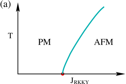
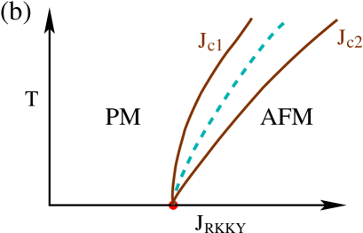
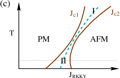
Figure 1: (a) Hypothetical phase diagram of the periodic Anderson model [see Eq.(2) below]. There is a continuous phase transition between the PM and AFM phases and it ends up with a QCP. (b) and (c) Two scenarios of the EDMFT phase transition, which was found to be first order at $T>0$ si3 (11, 12, 13). In the figures, the $J_{c1}$ line is where the AFM solution disappears. At the locus there is a finite jump in the magnetization which decreases with decreasing temperature ping (12, 11). The $J_{c2}$ line is where the spin susceptibility at the AFM ordering wave vector diverges. In the region in between the two phases coexist and the first order transition is represented by a dashed curve. Panel (c) is a sketch of the results presented in Ref.ping (12). According to the calculation, the Kondo temperature $T_{K}$ is near the location where the $J_{c1}$ and $J_{c2}$ lines become closest. The lowest temperature reached in Ref.ping (12) is $T=0.25T_{K}$, which is represented by a horizontal dotted line in (c).

EDMFT has been applied to study the heavy Fermions via the Kondo si0 (6, 9, 10, 11) and Anderson lattice ping (12) models. Early EDMFT studies si0 (6, 9, 10) approached the heavy Fermion quantum phase transition (QPT) by following the paramagnetic (PM) solution until where it ceased to exist and the spin susceptibility diverged. However, the absence of the AFM phase in this scenario makes it difficult to judge if the critical behavior is associated with a continuous transition or the spinodal point of a first order transition. To clarify this important issue, numerical studies of the phase transition from both the PM and AFM sides were carried out at finite temperatures si3 (11, 12). In the solution of the periodic Anderson model (PAM) ping (12), two different transitions were found ($J_{c1}$ and $J_{c2}$ lines defined in Fig.1) which bounded a region where the PM and AFM phases coexisted. Similar behavior was also found in the solution based on the Kondo lattice model si3 (11, 13). This strongly indicates a first order phase transition, at least for $T>0$.

There are important questions, though, remain unanswered. First, given the totally different behaviors along the mean field transition lines, it is interesting to compare and contrast the physical meanings of the two. Unlike at the $J_{c2}$ line where the spin susceptibility at the AFM ordering wave vector becomes critical, it is unclear from the EDMFT calculation itself si3 (11, 12) which response function is driven critical, even though critical slowing down was experienced. Second, there are concerns with regard to a possible quantum critical point (QCP) where the $J_{c1}$ and $J_{c2}$ lines merge [see Fig.1(b)]. As a result, a novel quantum critical behavior may occur. Existing analysis pankov (14) can not rule out such a possibility. Besides, although our numerical results with $T\geq 0.25T_{K}$ does not seem to support this scenario [see Fig.1(c)], the temperatures reached in Ref.ping (12) may not be low enough to be conclusive. The current paper is contributed to clarify these issues, which are all related to the local spin self-energy approximation.

In Sec.II we introduce the EDMFT approximation on two sublattices via Baym-Kadanoff functional which is then used in Sec.III to formulate the instability criteria. Technical details of these two parts are presented in Appendices A and B, respectively. Sec.IV contains conclusions and further discussions.

II EDMFT Formulation of the Periodic Anderson Model

II.1 The Periodic Anderson Model

We study the periodic Anderson model (PAM) with the local f-moments forming a hypercubic lattice in $d$-dimensions:

$$H=\sum_{\vec{k}\sigma}(\epsilon_{\vec{k}}-\mu)c^{\dagger}_{\vec{k}\sigma}c_{\vec{k}\sigma}+V\sum_{i\sigma}(c_{i\sigma}^{\dagger}f_{i\sigma}+f_{i\sigma}^{\dagger}c_{i\sigma})+(E_{f}-\mu)\sum_{i\sigma}n^{f}_{i\sigma}$$

$$+U\sum_{i}\left(n^{f}_{i\uparrow}-1/2\right)\left(n^{f}_{i\downarrow}-1/2\right)+\frac{J_{RKKY}}{d}\sum_{\langle ij\rangle}S^{f}_{i,z}S^{f}_{j,z}.$$ (2)

An RKKY interaction is introduced explicitly between the z-components of the nearest-neighboring f-electron spins, $S^{f}_{i,z}=n^{f}_{i,\uparrow}-n^{f}_{i,\downarrow}$. After intergrating out the c-electrons and introducing a Hubbard-Stratonovic field $\phi$ to decouple the interactions, we obtain:

$${\cal A}=-\int_{0}^{\beta}d\tau\int_{0}^{\beta}d\tau^{\prime}\sum_{ii^{\prime},\sigma}f^{\dagger}_{\sigma}(i,\tau)\left[G_{0\sigma}\right]^{-1}(i\tau|i^{\prime}\tau^{\prime})f_{\sigma}(i^{\prime},\tau^{\prime})$$

$$-\frac{1}{2}\int_{0}^{\beta}d\tau\int_{0}^{\beta}d\tau^{\prime}\sum_{ii^{\prime}}\phi(i,\tau)[D_{0}]^{-1}(i\tau|i^{\prime}\tau^{\prime})\phi(i^{\prime},\tau^{\prime})-\int_{0}^{\beta}d\tau\sum_{i}\phi(i,\tau)S^{f}_{z}(i,\tau).$$ (3)

In this action the hybridization broadened f-band is described by the free Green’s function:

$$G_{0}(\vec{k},ip_{n})=\left(ip_{n}+\mu-E_{f}-\frac{V^{2}}{ip_{n}+\mu-\epsilon_{\vec{k}}}\right)^{-1}$$ (4)

with $p_{n}=(2n+1)\pi/\beta$. The free Boson Green’s function is given by:

$$D_{0}(\vec{k},i\omega_{n})=D_{0}(\vec{k})=-U+\frac{J_{RKKY}}{d}\sum_{i=1}^{d}\cos k_{i}$$ (5)

with $\omega_{n}=2n\pi/\beta$. Since the bare interaction is instantaneous, the r.h.s. of Eq.(5) is frequency independent.

II.2 EDMFT via Baym-Kadanoff Formulation

We formulate the EDMFT via Baym-Kadanoff functional chitra (8):

$$\Gamma_{BK}[G,D,m]={\rm Tr\;}\ln G-{\rm Tr\;}G_{0}^{-1}G-\frac{1}{2}{\rm Tr\;}\ln D+\frac{1}{2}{\rm Tr\;}D_{0}^{-1}D$$

$$+\frac{1}{2}mD_{0}^{-1}m+\Phi_{EDMFT}[G_{loc},D_{loc},m],$$ (6)

$G$ ($D$) is the full electron (Boson) Green’s function. $m=\langle\phi\rangle$. The EDMFT approximated potential $\Phi_{EDMFT}$ is a two particle irreducible (2PI) functional of the local Green’s functions only. Since the action (3) contains just a spatially local interaction vertex, $\Phi_{EDMFT}$ can be written as a summation over the local contributions. On a bipartite lattice with sublattices $A$ and $B$, this potential is given by:

$$\Phi_{EDMFT}[G_{loc},D_{loc},m]=-\int_{0}^{\beta}d\tau\sum_{j,\sigma}m(j,\tau)\sigma G_{\sigma}(j\tau^{-}|j\tau)+\sum_{j\in A}\Psi_{A}[G_{jj,\sigma},D_{jj}]+\sum_{l\in B}\Psi_{B}[G_{ll,\sigma},D_{ll}]$$ (7)

where the functionals $\Psi$ contain second and higher order diagrams in terms of the interaction vertex. To solve the AFM phase with the single impurity EDMFT, we need to further assume (see Ref.ping (12)),

$$\Psi_{A}[G_{jj,\sigma},D_{jj}]_{j\in A}=\Psi_{B}[G_{ll,-\sigma},D_{ll}]_{l\in B}$$ (8)

Here the translational invariance within each sublattice is utilized. In the PM phase the electron Green’s functions are spin independent and the assumption is still valid.

The Baym-Kadanoff functional gives physical solution at its stationary point. As a result, we have,

$$\left[G_{\sigma}^{-1}(\vec{k},ip_{n})\right]_{AB}=\left(\begin{array}[]{cc}ip_{n}+\mu-E_{f}&0\\ 0&ip_{n}+\mu-E_{f}\end{array}\right)$$

$$-\frac{V^{2}}{(ip_{n}+\mu)^{2}-\epsilon^{2}_{\vec{k}}}\left(\begin{array}[]{cc}ip_{n}+\mu&-\epsilon_{\vec{k}}\exp(+ik_{x})\\ -\epsilon_{\vec{k}}\exp(-ik_{x})&ip_{n}+\mu\\ \end{array}\right)-\left(\begin{array}[]{cc}\Sigma_{\sigma}(ip_{n})&0\\ 0&\Sigma_{-\sigma}(ip_{n})\end{array}\right).$$ (9)

$$D^{-1}(\vec{k},i\omega_{n})=D_{0}^{-1}(\vec{k})-\Pi(i\omega_{n})$$ (10)

$$m(i,\tau)=\sum_{j,\sigma}D_{0,ij}\sigma\langle f_{\sigma}^{\dagger}(j,\tau)f_{\sigma}(j,\tau)\rangle$$ (11)

Several remarks are in place. First, due to the sublattice structure, the electron Dyson equation (9) is in a $2\times 2$ matrix form. The electron self energy,

$$\Sigma_{X,\sigma}(ip_{n})\stackrel{{\scriptstyle\rm def}}{{=}}\frac{\delta\Phi_{EDMFT}}{\delta G_{jj,\sigma}(ip_{n})}|_{j\in X},$$ (12)

with $X=A,B$, is local in space. Due to translational invariance, we can neglect its spatial coordinates. From Eq.(8),

$$\Sigma_{A,\sigma}(ip_{n})=\Sigma_{B,-\sigma}(ip_{n}).$$ (13)

As a result note-spin (15), we are allowed to suppress the sublattice index of the self-energy in Eq.(9). In the PM phase, the self-energies are spin independent and the equation reduces to:

$$G^{-1}(\vec{k},ip_{n})=G_{0}^{-1}(\vec{k},ip_{n})-\Sigma(ip_{n}).$$ (14)

Second, in the Boson Dyson equation (10), the self-energy is defined as:

$$\Pi_{X}(i\omega_{n})\stackrel{{\scriptstyle\rm def}}{{=}}-2\frac{\delta\Phi_{EDMFT}}{\delta D_{jj}(i\omega_{n})}|_{j\in X}.$$ (15)

Eq.(10) carries a scalar form because the local Boson self-energy is the same on both sublattices due to symmetry. Finally, from Eq.(11), the physical order parameter $m$ is time independent and its momentum dependence, according to Eq.(8), is restricted to $\vec{Q}\stackrel{{\scriptstyle\rm def}}{{=}}(\pi,\cdots,\pi)$ for both the AFM ($m\neq 0$) and the PM ($m=0$) phases. In EDMFT, we solve the self-energies using an effective impurity model under certain self-consistent conditions.. [See Appendix A]

III Instability Criteria

III.1 Instability Criterion of the AFM phase ($J_{c1}$ line)

The general instability criterion against the formation or disappearance of a static spin density wave of wave vector $\vec{Q}$ is given by:

$$\chi^{-1}\stackrel{{\scriptstyle\rm def}}{{=}}\frac{d^{2}\Gamma_{BK}[G,D,m]}{dm^{*}dm}=0.$$ (16)

where $m=m(\vec{Q},i0)$. Here the total derivatives are taken on the physical manifold of the Baym-Kadanoff functional defined through Eqs.(9)-(11). As a result, the criterion becomes, (see Appendix B for details)

$$\chi^{-1}_{J_{c1}}\stackrel{{\scriptstyle\rm def}}{{=}}D_{0}^{-1}(\vec{Q})-\int_{0}^{\beta}d\tau\sum_{a,b=1}^{2}(-1)^{a+b}\Pi_{J_{c1},\vec{Q}}[(\tau|\tau),(0|0)]=0$$ (17)

where

$$\bigglb[\Pi_{J_{c1},\vec{Q}}\biggrb]^{-1}[(\tau_{1}|\tau_{1}^{\prime}),(\tau_{2}|\tau_{2}^{\prime})]=\bigglb[\chi_{0,\vec{Q}}^{-1}-\chi_{0,imp}^{-1}+\chi_{imp}^{-1}+\tilde{\cal D}_{0}\biggrb][(\tau_{1}|\tau_{1}^{\prime}),(\tau_{2}|\tau_{2}^{\prime})]$$ (18)

In the above equation $\chi_{0,\vec{Q}}$ is an electron-hole bubble evaluated with the full Green’s functions at the wave vector $\vec{Q}$. $\chi_{0,imp}$ is a smiliar bubble obtained via the full impurity Green’s function. $\chi_{imp}$ is a four point response function of the impurity model. $\tilde{\cal D}_{0}$, which depends on ${\cal D}_{0}$, is the bare interaction in the impurity model. Eq.(17) gives the general EDMFT instability criterion without further approximation and applies to the $J_{c1}$ line where the AFM solution at $\vec{Q}=(\pi,\cdots,\pi)$ disappears. The existence of the electron-hole bubble at the ordering wave vector in Eq.(18) reveals the fact that even in the infinite coordination limit where the mean field method becomes exact, there is still a non-vanishing momentum-dependent contribution in the effective spin susceptibility. The matrix inversions in Eq.(18) involve matrices labeled by four time coordinates, two for the row and two for the column, respectively. As a result, this expression is generally very complicated and can not be further simplified.

III.2 Instability Criterion of the PM phase ($J_{c2}$ line)

In the EDMFT of the PM phase, the effective susceptibility given in Eq.(18) contributes directly to the spin self-energy pankov (14) and, as a result, should be local in space. This means we need further to restrict $\chi_{0}$ to be local. However, from the EDMFT self-consistency that the local Green’s functions on the lattice equal to the impurity ones, $\chi_{0,loc}$=$\chi_{0,imp}$. Hence the instability criterion becomes

$$\chi^{-1}_{J_{c2}}\stackrel{{\scriptstyle\rm def}}{{=}}D_{0}^{-1}(\vec{Q})-\int_{0}^{\beta}d\tau\sum_{a,b=1}^{2}(-1)^{a+b}\Pi_{J_{c2}}[(\tau|\tau),(0|0)]=0$$ (19)

where

$$\bigglb[\Pi_{J_{c2}}\biggrb]^{-1}[(\tau_{1}|\tau_{1}^{\prime}),(\tau_{2}|\tau_{2}^{\prime})]=\bigglb[\chi_{imp}^{-1}+\tilde{\cal D}_{0}\biggrb][(\tau_{1}|\tau_{1}^{\prime}),(\tau_{2}|\tau_{2}^{\prime})]$$ (20)

The special form of the matrix ${\cal D}_{0}$ [see Eq.(39)] allows us to carry out the matrix operations explicitly and obtain,

$$D_{0}(\vec{Q})={\cal D}_{0}(i0)+\chi_{zz}^{-1}(i0)=\Pi^{-1}(i0)$$ (21)

with

$$\chi_{zz}(\tau)\stackrel{{\scriptstyle\rm def}}{{=}}\langle S_{z}^{f}(\tau)S_{z}^{f}(0)\rangle\equiv[\chi_{imp,G_{\uparrow}G_{\uparrow}}-\chi_{imp,G_{\uparrow}G_{\downarrow}}-\chi_{imp,G_{\downarrow}G_{\uparrow}}+\chi_{imp,G_{\downarrow}G_{\downarrow}}][(\tau|\tau),(0|0)]$$ (22)

The last equality in Eq.(21) is derived by an identity identity (16). Comparing with the Boson Dyson equation (10), we see that the above instability criterion is identical to the Stoner criterion in which the divergence of the magnetic susceptibility at $\vec{Q}=(\pi,\cdots,\pi)$ signals phase transition note (17).

IV Conclusions and Discussions

We have derived in this paper the phase instability criterion of the EDMFT solution to the periodic Anderson model for both the AFM and PM phases. The generic instability criterion (which applies to $J_{c1}$ line in Fig.1) involves an effective spin susceptibility, Eq.(17), and is different from that used to determine the transition line ($J_{c2}$) bounding the PM phase, Eq.(19). The difference is in an extra electron-hole bubble at the AFM ordering wave-vector in the former. This bubble is momentum dependent and survives in the infinite coordination limit. As a result, at the locus where one of the phases reaches the instability condition, the other one remains stable. This explains the phase coexistence. It persists to $T=0$ since the electron-hole bubble remains non-zero. This is consistent with what we obtained numerically ping (12) in Region II of Fig.1(c). We should point out, though, at dimensions $d>4$ and temperatures $T\gtrsim T_{Kondo}$ [Region I in Fig.1(c)], the difference between the $J_{c1}$ and $J_{c2}$ lines becomes negligibly small ping1 (18). This is due to the spatial correlation becoming weaker at higher dimensions pankov (14) and temperatures. We note in passing that no matter which criterion is satisfied, the divergence of the corresponding effective spin susceptibility at the AFM ordering wave vector naturally results in the divergence of the local spin susceptibility as long as the spin fluctuations are two dimensional si0 (6, 12). This is a result of the dimensionality and has nothing to do with the spin self-energy being local in space.

The true mean field transition is thus first order and lies between the $J_{c1}$ and $J_{c2}$ lines where the free energies of the two phases cross. Physically, the two sublattice EDMFT (as applied in the AFM phase) contains in its instability criterion an electron-hole bubble, which serves as a rough description of the feedback from the electron-hole excitations to the spin response. However, this feedback does not appear explicitly in the EDMFT self-consistency, which is evident from what we described in Appendix A. As a result, the EDMFT spin susceptibility, which is different from the physical one in the instability criterion, Eq.(17), does not experience any singularity as the $J_{c1}$ line is crossed. On the other hand, the homogeneous EDMFT (as applied in the PM phase), contains the same singular behavior in the spin response as that in the instability criterion, Eq.(19). As a result, when the phase boundary is approached, EDMFT is able to adjust self-consistently to reflect the singular behavior in the spin channel. However, as we have already noted, the problem on this side is that the feedback from the non-local electron-hole excitations is totally missing. So both the transition lines contain unphysical features, and neither of them, as far as the critical properties are concerned, is close to the true transition. A related issue, which concerns the critical exponent $\alpha$ in Eq.(1) along the $J_{c2}$ line, further supports our conclusion. It was shown that at $T=0$ on the $J_{c2}$ line, the critical frequency dependence could not develop a sublinear form pankov1 (19).

After all, it is not a surprise that, although it works well qualitatively in describing many other physical properties ping (12), the EDMFT fails to capture the right phase transition. This is certainly one of the issues one needs to improve over the mean field approach. Given what we have concluded in this paper, it seems important that one needs to find a way allowing proper feedback from the electron-hole excitations, which is spatially non-local, to the f-electron spin response. A natural way to proceed is to combine the EDMFT scheme with the random phase approximation (RPA) ping2 (20). In this combination, the spin self-energy contains the local EDMFT part together with the non-local RPA part. This is a desirable feature as one can see from the EDMFT instability criterion Eq.(18). Besides, the scheme is derivable from the Baym-Kadanoff functional ping2 (20). Of course, with the new scheme, the instability criterion itself is modified and its implication to the heavy Fermion phase transition has not yet been explored. A different route is to utilize the cellular DMFT cdmft (21). To this end, a two impurity Anderson model subject to the DMFT self-consistent electron bath results in a qualitative improvement ping3 (22). In this formalism, the RKKY interaction is generated dynamically, instead of being added in by hand as in Eq.(2). The spin susceptibility across the two impurity sites, which contains the corresponding electron-hole bubble as the lead order contribution, renders a limited momentum dependence and turns out to be essential to the improvement.

Appendix A Effective Impurity Model and EDMFT Self-Consistency

To obtain the local self-energies, we need to solve an effective impurity model:

$${\cal A}_{0}^{eff}=-\int_{0}^{\beta}d\tau\int_{0}^{\beta}d\tau^{\prime}\sum_{\sigma}f^{\dagger}_{\sigma}(0,\tau)\left[{\cal G}_{0\sigma}\right]^{-1}(\tau-\tau^{\prime})f_{\sigma}(0,\tau^{\prime})$$

$$-\frac{1}{2}\int_{0}^{\beta}d\tau\int_{0}^{\beta}d\tau^{\prime}\phi(0,\tau){\cal D}_{0}^{-1}(\tau-\tau^{\prime})\phi(0,\tau^{\prime})-\int_{0}^{\beta}d\tau\phi(0,\tau)S^{f}_{z}(0,\tau).$$ (23)

The mean field Weiss functions ${\cal G}_{0\sigma}$ and ${\cal D}_{0}$ are decided by the following self-consistent conditions:

$${\cal G}^{-1}_{0\sigma}(ip_{n})=[\sum_{\vec{k}}G_{\sigma}(k,ip_{n})]^{-1}+\Sigma^{imp}_{\sigma}(ip_{n})$$ (24)

$${\cal D}^{-1}_{0}(i\omega_{n})=[\sum_{\vec{k}}D_{\sigma}(\vec{k},i\omega_{n})]^{-1}+\Pi^{imp}(i\omega_{n})$$ (25)

with $G_{\sigma}(\vec{k},ip_{n})$ and $D_{\sigma}(\vec{k},i\omega_{n})$ given by Eqs.(9) and (10), respectively. The self-energies are,

$$\Sigma^{imp}_{\sigma}(ip_{n})=[{\cal G}_{0\sigma}]^{-1}(ip_{n})-[G^{imp}_{\sigma}]^{-1}(ip_{n})$$ (26)

$$\Pi^{imp}(i\omega_{n})=[{\cal D}_{0}]^{-1}(i\omega_{n})-[D^{imp}]^{-1}(i\omega_{n})$$ (27)

where the impurity Green’s functions $G^{imp}_{\sigma}$ and $D^{imp}$ are obtained by solving the effective action (23). In Eqs.(9) and (10), we need to use the lattice self-energies which are usually assumed to be the same as the impurity ones in the disordered phase. In the ordered phase, the electron self-energy on the lattice is different from that of the impurity model by a Hartree term, while the Boson self-energy is still the same,

$$\Sigma_{\sigma}(ip_{n})=\Sigma^{imp}_{\sigma}(ip_{n})-\sigma[{\cal D}_{0}(i0)-(U-J_{RKKY})]\langle S_{z}^{f}\rangle$$ (28)

$$\Pi(i\omega_{n})=\Pi^{imp}(i\omega_{n})$$ (29)

The meaning of Eq.(28) is that we need to replace the Hartree self-energy of the impurity model by that on the lattice, using the electron magnetization. This procedure is related to Eq.(11), which would otherwise introduce a third self-consistent equation. With this, we have presented a complete self-consistent loop.

Appendix B Derivation of the Instability Criterion for the AFM phase

We derive here the instability criterion specific to the periodic Anderson model. From the general condition, Eq.(16), together with Eqs.(9)-(11), we obtain,

$$\frac{\partial^{2}\Gamma_{BK}}{\partial m^{*}\partial m}+\int dx\frac{\partial G_{\sigma_{x}}(x)}{\partial m^{*}}\frac{\partial^{2}\Gamma_{BK}}{\partial G_{\sigma_{x}}(x)\partial m}+\int dx\frac{\partial D(x)}{\partial m^{*}}\frac{\partial^{2}\Gamma_{BK}}{\partial D(x)\partial m}=0$$ (30)

$$\int dx\frac{\partial G_{\sigma_{x}}(x)}{\partial m^{*}}\frac{\partial^{2}\Gamma_{BK}}{\partial G_{\sigma_{x}}(x)\partial G_{\sigma_{y}}(y)}+\int dx\frac{\partial D(x)}{\partial m^{*}}\frac{\partial^{2}\Gamma_{BK}}{\partial D(x)\partial G_{\sigma_{y}}(y)}+\frac{\partial^{2}\Gamma_{BK}}{\partial m^{*}\partial G_{\sigma_{y}}(y)}=0$$ (31)

$$\int dx\frac{\partial G_{\sigma_{x}}(x)}{\partial m^{*}}\frac{\partial^{2}\Gamma_{BK}}{\partial G_{\sigma_{x}}(x)\partial D(y)}+\int dx\frac{\partial D(x)}{\partial m^{*}}\frac{\partial^{2}\Gamma_{BK}}{\partial D(x)\partial D(y)}+\frac{\partial^{2}\Gamma_{BK}}{\partial m^{*}\partial D(y)}=0.$$ (32)

We used $x=(\vec{R}_{j},\tau|\vec{R}_{j^{\prime}},\tau^{\prime})$, (similar for $y$) and $\int dx=\sum_{j,j^{\prime}}\int_{0}^{\beta}d\tau\int_{0}^{\beta}d\tau^{\prime}$. Summation over the repeated spin indices is implied. Solving $\partial G/\partial m^{*}$ and $\partial D/\partial m^{*}$ from Eqs.(31) and (32), and substituting them in Eq.(30), we obtain:

$$\frac{\partial^{2}\Gamma_{BK}[G,D,m]}{\partial m^{*}\partial m}-\int dx\int dy\left[\partial^{2}\Gamma_{BK}/\partial m^{*}\partial G_{\sigma_{x}}(x),\partial^{2}\Gamma_{BK}/\partial m^{*}\partial D(x)\right]$$

$$\times\left[\begin{array}[]{cc}\partial^{2}\Gamma_{BK}/\partial G_{\sigma_{x}}\partial G_{\sigma_{y}}&\partial^{2}\Gamma_{BK}/\partial G_{\sigma_{x}}\partial D\\ \partial^{2}\Gamma_{BK}/\partial D\partial G_{\sigma_{y}}&\partial^{2}\Gamma_{BK}/\partial D\partial D\end{array}\right]^{-1}(x,y)\left[\begin{array}[]{c}\partial^{2}\Gamma_{BK}/\partial G_{\sigma_{y}}(y)\partial m\\ \partial^{2}\Gamma_{BK}/\partial D(y)\partial m\end{array}\right]=0.$$ (33)

Using Eqs.(6) and (7), we find $\partial^{2}\Gamma_{BK}/\partial G_{\sigma}(j\tau_{1}|j^{\prime}\tau_{1}^{{}^{\prime}})\partial m(i,\tau)=-\sigma\delta_{ij}\delta_{ij^{\prime}}\delta(\tau-\tau_{1})\delta(\tau-\tau_{1}^{{}^{\prime}})$ and $\partial^{2}\Gamma_{BK}/\partial D(j\tau_{1}|j^{\prime}\tau_{1}^{{}^{\prime}})\partial m(i,\tau)=0$. Besides, $\partial^{2}\Gamma_{BK}[G,D,m]/\partial m^{*}\partial m=D_{0}^{-1}(\vec{Q})$. So we have:

$$\beta D_{0}^{-1}(\vec{Q})=\frac{1}{N}\sum_{j_{1}}\int_{0}^{\beta}d\tau_{1}\sum_{j_{2}}\int_{0}^{\beta}d\tau_{2}\exp(-i\vec{Q}\cdot\vec{R}_{j_{1}})\exp(i\vec{Q}\cdot\vec{R}_{j_{2}})$$ (34)

$$\times(1,-1,0)\left[\begin{array}[]{ccc}\Gamma^{(2)}_{G_{\uparrow}G_{\uparrow}}&\Gamma^{(2)}_{G_{\uparrow}G_{\downarrow}}&\Gamma^{(2)}_{G_{\uparrow}D}\\ \Gamma^{(2)}_{G_{\downarrow}G_{\uparrow}}&\Gamma^{(2)}_{G_{\downarrow}G_{\downarrow}}&\Gamma^{(2)}_{G_{\downarrow}D}\\ \Gamma^{(2)}_{DG_{\uparrow}}&\Gamma^{(2)}_{DG_{\downarrow}}&\Gamma^{(2)}_{DD}\end{array}\right]^{-1}[(j_{1}\tau_{1}|j_{1}\tau_{1}),(j_{2}\tau_{2}|j_{2}\tau_{2})]\left(\begin{array}[]{r}1\\ -1\\ 0\end{array}\right),$$

with $\Gamma^{(2)}_{XY}[(j_{1}\tau_{1}|j_{1}^{\prime}\tau_{1}^{\prime}),(j_{2}\tau_{2}|j_{2}^{\prime}\tau_{2}^{\prime})]=\partial^{2}\Gamma_{BK}/\partial X(j_{1}\tau_{1}|j_{1}^{\prime}\tau_{1}^{\prime})\partial Y(j_{2}\tau_{2}|j_{2}^{\prime}\tau_{2}^{\prime})$ for $X,Y=G_{\sigma},D$. To solve the matrix $\Gamma^{(2)}$, we use again the Baym-Kadanoff functional (6) and obtain:

$$\Gamma^{(2)}_{XY}[(j_{1}\tau_{1}|j_{1}^{\prime}\tau_{1}^{\prime}),(j_{2}\tau_{2}|j_{2}^{\prime}\tau_{2}^{\prime})]=\chi_{0,XY}^{-1}[(j_{1}\tau_{1}|j_{1}^{\prime}\tau_{1}^{\prime}),(j_{2}\tau_{2}|j_{2}^{\prime}\tau_{2}^{\prime})]+\Phi^{(2)}_{XY}[(j_{1}\tau_{1}|j_{1}^{\prime}\tau_{1}^{\prime}),(j_{2}\tau_{2}|j_{2}^{\prime}\tau_{2}^{\prime})]$$ (35)

where

$$\chi_{0,XY}[(j_{1}\tau_{1}|j_{1}^{\prime}\tau_{1}^{\prime}),(j_{2}\tau_{2}|j_{2}^{\prime}\tau_{2}^{\prime})]\stackrel{{\scriptstyle\rm def}}{{=}}\left\{\begin{array}[]{cc}-G_{\sigma_{X^{\prime}},\sigma_{Y}}(j_{1}^{\prime}\tau_{1}^{\prime}|j_{2}\tau_{2})G_{\sigma_{Y^{\prime}},\sigma_{X}}(j_{2}^{\prime}\tau_{2}^{\prime}|j_{1}\tau_{1}),&X,Y=G_{\sigma}\\ D(j_{1}\tau_{1}|j_{2}\tau_{2})D(j_{1}^{\prime}\tau_{1}^{\prime}|j_{2}^{\prime}\tau_{2}^{\prime})+D(j_{1}\tau_{1}|j_{2}^{\prime}\tau_{2}^{\prime})D(j_{1}^{\prime}\tau_{1}^{\prime}|j_{2}\tau_{2}),&X,Y=D\\ 0,&{\rm else}\end{array}\right.$$ (36)

$$\Phi^{(2)}_{XY}[(j_{1}\tau_{1}|j_{1}^{\prime}\tau_{1}^{\prime}),(j_{2}\tau_{2}|j_{2}^{\prime}\tau_{2}^{\prime})]\stackrel{{\scriptstyle\rm def}}{{=}}\frac{\partial^{2}\Phi_{EDMFT}}{\partial X(j_{1}\tau_{1}|j_{1}^{\prime}\tau_{1}^{\prime})\partial Y(j_{2}\tau_{2}|j_{2}^{\prime}\tau_{2}^{\prime})}$$ (37)

$\Phi^{(2)}_{XY}$, same as $\Phi_{EDMFT}$, contains only propagators local in space and is 2PI in separating the external legs labeled by 1 and 1’ from those 2 and 2’. It follows then pankov (14),

$$\bigglb[\Phi^{(2)}\biggrb]_{XY}[(j_{1}\tau_{1}|j_{1}^{\prime}\tau_{1}^{\prime}),(j_{2}\tau_{2}|j_{2}^{\prime}\tau_{2}^{\prime})]=\delta_{j_{1},j_{1}^{\prime}}\delta_{j_{1},j_{2}}\delta_{j_{1},j_{2}^{\prime}}\bigglb[-\chi_{0,imp}^{-1}+\chi_{imp}^{-1}+\tilde{\cal D}_{0}\biggrb]_{XY}[(\tau_{1}|\tau_{1}^{\prime}),(\tau_{2}|\tau_{2}^{\prime})].$$ (38)

Here $\chi_{0,imp}$ is similar to that defined in Eq.(36) except being local in space. We also defined:

$$\tilde{\cal D}_{0}[(\tau_{1}|\tau_{1}^{\prime}),(\tau_{2}|\tau_{2}^{\prime})]\stackrel{{\scriptstyle\rm def}}{{=}}\delta(\tau_{1}-\tau_{1}^{\prime})\delta(\tau_{2}-\tau_{2}^{\prime})\left[\begin{array}[]{ccc}\;\;{\cal D}_{0}(\tau_{1}-\tau_{2})&-{\cal D}_{0}(\tau_{1}-\tau_{2})&0\\ -{\cal D}_{0}(\tau_{1}-\tau_{2})&\;\;{\cal D}_{0}(\tau_{1}-\tau_{2})&0\\ 0&0&0\end{array}\right]$$ (39)

$$\chi_{imp,XY}[(0\tau_{1}|0\tau_{1}^{\prime}),(0\tau_{2}|0\tau_{2}^{\prime})]\stackrel{{\scriptstyle\rm def}}{{=}}\langle T_{\tau}\;:\hat{\cal O}_{X}^{\dagger}(0,\tau_{1})\hat{\cal O}_{X}(0,\tau_{1}^{\prime})::\hat{\cal O}_{Y}^{\dagger}(0,\tau_{2})\hat{\cal O}_{Y}^{\dagger}(0,\tau_{2}^{\prime}):\rangle$$ (40)

where $\hat{\cal O}_{X}=c_{\sigma}$ ($\phi$) if $X=G_{\sigma}$ ($D$). The instability criterion becomes:

$$D_{0}^{-1}(\vec{Q})=\frac{1}{N}\sum_{j_{1},j_{2}}\int_{0}^{\beta}d\tau\exp(-i\vec{Q}\cdot\vec{R}_{j_{1}})\exp(i\vec{Q}\cdot\vec{R}_{j_{2}})$$

$$\sum_{a,b=1}^{2}(-1)^{a+b}\left[\chi_{0}^{-1}-\chi_{0,imp}^{-1}+\chi_{imp}^{-1}+\tilde{\cal D}_{0}\right]_{a,b}^{-1}[(j_{1}\tau|j_{1}\tau),(j_{2}0|j_{2}0)].$$ (41)

where all the four terms in the square parenthesis are $3\times 3$ matrices and after matrix inversion, only the first $2\times 2$ block contributes. It should be noted that the matrices are also labeled by the two pairs of the space-time coordinates and any matrix operation should take these into account. As a result, e.g., in Eq.(41) the full matrix, labeled by $[(j_{1}\tau_{1}|j_{1}^{\prime}\tau_{1}^{\prime}),(j_{2}\tau_{2}|j_{2}^{\prime}\tau_{2}^{\prime})]$, should be inverted first and only after that, we set the labels to be $[(j_{1}\tau|j_{1}\tau),(j_{2}0|j_{2}0)]$.

Finally, since in Eq.(41), $\chi_{0}$ is the only term contains spatially non-local contributions, the Fourier transform over the lattice coordinate can be taken into the matrix inversion, which gives:

$$D_{0}^{-1}(\vec{Q})=\int_{0}^{\beta}d\tau\sum_{a,b=1}^{2}(-1)^{a+b}\chi_{J_{c1},\vec{Q}}[(\tau|\tau),(0|0)]$$ (42)

where

$$\bigglb[\chi_{J_{c1},\vec{Q}}\biggrb]^{-1}[(\tau_{1}|\tau_{1}^{\prime}),(\tau_{2}|\tau_{2}^{\prime})]=\bigglb[\chi_{0,\vec{Q}}^{-1}-\chi_{0,imp}^{-1}+\chi_{imp}^{-1}+\tilde{\cal D}_{0}\biggrb][(\tau_{1}|\tau_{1}^{\prime}),(\tau_{2}|\tau_{2}^{\prime})]$$ (43)

This gives an instability criterion consistent with the EDMFT Baym-Kadanoff functional, Eqs.(6) and (7), without any further approximation.

As it turns out, we need further to assume $\chi_{0}$ be spatially local in Eq.(41), in order to describe the PM phase. In such a case, $\chi_{0}\rightarrow\chi_{0,loc}$, we have (1) the momentum dependent phase factors in Eq.(41) cancel out and (2) $\chi_{0,imp}$ cancels $\chi_{0,loc}$ due to the EDMFT self-consistency that the local lattice Green’s functions equal to the impurity ones.

References

• (1) S. Doniach, Physica B 91, 231 (1977).
• (2) C. M. Varma, Rev. Mod. Phys. 48, 219 (1976).
• (3) G. R. Stewart, Rev. Mod. Phys. 73, 797 (2001).
• (4) H. von Lohneysen, J. Phys.: Cond. Matt 8, 9689 (1996).
• (5) A. Schroder, et. al., Nature, 407, 351 (2000).
• (6) Q. Si, S. Rabello, K. Ingersent, and J. L. Smith, Nature, 413, 804 (2001).
• (7) S. Sachdev and J. Ye, Phys. Rev. Lett. 70, 3339 (1993); H. Kajueter, Ph.D. thesis, Rutgers University (1996); Q. Si and J. L. Smith, Phys. Rev. Lett. 77, 3391 (1996); J. L. Smith and Q. Si, Phys. Rev. B 61, 5184 (2000).
• (8) R. Chitra and G. Kotliar, Phys. Rev. B 63, 115110 (2001).
• (9) L. Zhu and Q. Si, Phys. Rev. B 66, 024426 (2002); G. Zarand and E. Demler, Phys. Rev. B 66, 024427 (2002).
• (10) D. R. Grempel and Q. Si, Phys. Rev. Lett. 91, 026401 (2003).
• (11) J.-X. Zhu, D. R. Grempel, and Q. Si, Phys. Rev. Lett. 91, 156404 (2003).
• (12) P. Sun and G. Kotliar, Phys. Rev. Lett. 91, 037209 (2003).
• (13) Q. Si, private communication.
• (14) S. Pankov, G. Kotliar, Y. Motome, Phys. Rev. B 66, 045117 (2002).
• (15) Given its form, Eq.(8) can also be interpreted, technically, as a Dyson equation for a system with spin-flip hoppings. In this picture, the instability criterion of the AFM phase, Eqs.(17) and (18), contains an extra, cross spin electron-hole bubble.
• (16) P. Sun and G. Kotliar Phys. Rev. B 66, 085120 (2002).
• (17) To see this point, one needs to remove β€œβˆ’Uπ‘ˆ-U” from both $D_{0}$ and Ξ βˆ’1superscriptΞ 1\Pi^{-1} identity (16). Since $\Pi(i0)<0$, it follows that the instability is first seen when $\vec{Q}=(\pi,\cdots,\pi)$.
• (18) P. Sun and G. Kotliar, unpublished.
• (19) S. Pankov, S. Florens, A. Georges, G. Kotliar, and S. Sachdev Phys. Rev. B 69, 054426 (2004).
• (20) P. Sun and G. Kotliar, Phys. Rev. Lett. 92, 196402 (2004).
• (21) G. Kotliar, S. Y. Savrasov, G. Palsson, and G. Biroli, Phys. Rev. Lett. 87, 186401 (2001).
• (22) P. Sun and G. Kotliar, cond-mat/0501176.