Nonequilibrium Kondo Effect in a Quantum Dot Coupled to Ferromagnetic Leads

Abstract

We study the Kondo effect in the electron transport through a quantum dot coupled to ferromagnetic leads, using a real-time diagrammatic technique which provides a systematic description of the nonequilibrium dynamics of a system with strong local electron correlations. We evaluate the theory in an extension of the ‘resonant tunneling approximation’, introduced earlier, by introducing the self-energy of the off-diagonal component of the reduced propagator in spin space. In this way we develop a charge and spin conserving approximation that accounts not only for Kondo correlations but also for the spin splitting and spin accumulation out of equilibrium. We show that the Kondo resonances, split by the applied bias voltage, may be spin polarized. A left-right asymmetry in the coupling strength and/or spin polarization of the electrodes significantly affects both the spin accumulation and the weight of the split Kondo resonances out of equilibrium. The effects are observable in the nonlinear differential conductance. We also discuss the influence of decoherence on the Kondo resonance in the frame of the real-time formulation.

I introduction

The continuing experimental progress with mesoscopic electronic devices has stimulated anew the interest in fundamental quantum mechanical questions ImryBook . A good example is the Kondo effect Hewson in electron transport through quantum dots (QD). The effect, which nowadays is well established experimentally GoldhaberGordon , has remained a challenging problem for nonequilibrium quantum transport theory  Hershfield0 ; Meir1 ; Meir2 ; Konig1 . After early experiments, which concentrated on semiconductor QDs, the Kondo effect was observed in single-atom Park and single-molecule transistors Liang , as well as in carbon nanotube QDs Nygard , all of which were coupled to metallic leads. More recently, the Kondo effect was demonstrated in QDs coupled to ferromagnetic leads Pasupathy ; Nygard1 . In this article, we will discuss the nonequilibrium Kondo effect in such systems as an example of the nontrivial collective many-body physics in magnetic nanostructures.

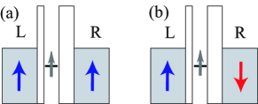
Figure 1: A single level quantum dot coupled to two ferromagnetic leads for (a) parallel and (b) antiparallel alignments of lead magnetizations. We allow for a left-right asymmetry in tunnel barriers and/or spin polarization factors.

Research on electronic properties in magnetic systems has evolved into an active field, “spintronics” Maekawabook . In spintronics devices magnetic properties control transport properties via the electron spin degree of freedom. One example is the tunnel magnetoresistance (TMR) in ferromagnetic tunnel junctions Miyazaki , which relies on switching the magnetization of the electrodes between parallel (P) and antiparallel (AP) orientations by an applied magnetic field. In magnetic multilayers, the intrinsic exchange coupling between layers Bruno1 influences the magnetic structure and consequently the transport properties Shinjo . The Kondo effect in transport through a QD coupled to ferromagnetic leads (Fig. 1) provides a prime example of many-body effects in spintronics devices. The theoretical model, a local spin coupled to two ferromagnetic leads, was originally introduced to explain the decrease of the TMR with increasing temperature Inoue . The model was revived recently, and led to a series of publications  Sergueev ; Martinek1 ; Dong ; PZhang ; Lopez ; Martinek2 ; MSChoi . In the early stage, due to different approximations used, the question remained controversial whether the Kondo resonance splits in the presence of spin-polarized leads Martinek1 ; Dong or not PZhang ; Lopez . The splitting was confirmed eventually by numerical-renormalization-group (NRG) techniques Martinek2 ; MSChoi .

The origin of the splitting of the Kondo resonances lies an exchange coupling induced by spin-dependent quantum charge fluctuations. Let us consider a single-level, originally spin-degenerate QD with energy $\epsilon_{0}\!<\!0$ (measured relative to the Fermi level of the lead electrons) and strong Coulomb interaction, $U\rightarrow\infty$. Then, double occupancy is suppressed and the QD behaves as a magnetic impurity. But there still exist quantum charge fluctuations due to the tunneling between the QD and the leads. An electron with majority-spin in the QD can tunnel between the QD and the leads easier than an electron with minority-spin, thus gaining a larger kinetic energy. As a result, a ferromagnetic exchange interaction between the QD spin and the lead magnetization is induced. It lifts the spin degeneracy of the QD level by $\Delta\epsilon$. Such a spin splitting quenches spin-flip scattering processes for low energies, below $|\Delta\epsilon|$, and suppresses the Kondo correlations. It also leads to a splitting of the Kondo resonance. The qualitative two-stage scaling theory presented in Ref. Martinek1 indicates that the high-energy part of quantum charge fluctuations, between $|\epsilon_{0}|$ and a cutoff energy $D$ (of the order of the itinerant electron band width) is responsible for a spin splitting given by

$$\Delta\epsilon\sim-P\frac{\Gamma}{\pi}\ln\frac{D}{|\epsilon_{0}|},\;\;\;\;\Gamma\!\equiv\!(\Gamma_{\uparrow}+\Gamma_{\downarrow})/2\,.$$ (1)

Here we assumed the coupling strength $\Gamma_{\sigma}$ between the QD level and the leads to be spin dependent. The splitting of the level results in a corresponding spin splitting of the Kondo peak in the spectral density. Remarkably, it is possible to compensate the spin splitting $\Delta\epsilon$ by applying an external magnetic field, and thus to recover the full Kondo effect Martinek1 .

In spite of the interest in the problem, a systematic approximation which can account for the spin splitting of the Kondo effect in nonequilibrium transport problems has not yet been presented.
- The NRG is a powerful tool for the investigation of the Kondo problem, but is limited to the equilibrium state. The validity of extensions to the nonequilibrium state Lopez ; Dong ; Martinek1 remains to be proven.
- The slave-boson mean-field approximation is correct in the limit of large degeneracy and able to capture the physics of the Kondo singlet at zero temperature Coleman . However, it does not account for the spin splitting since the description of quantum charge fluctuations is beyond mean-field theory.
- The non-crossing approximation (NCA), a systematic conserving approximation Kuramoto ; Bickers , has been successfully adopted to the nonequilibrium state Meir1 ; Meir2 . NCA accounts for spin-dependent quantum charge fluctuations and thus for the spin splitting due to ferromagnetic leads. But, it also generates an additional spurious peak at the Fermi level even in equilibrium Dong as well as a spurious peak in the presence of magnetic field Meir1 . Such a shortcoming is dangerous in the context of transport, which is sensitive to the electron states near the Fermi energy. The spurious peak can be made to disappear, if vertex corrections are properly accounted for Kroha . However, the generalization of NCA described in Ref. Kroha does not appear tractable in nonequilibrium situations.
- The equation-of-motion (EOM) approach, which was adopted in Ref. Martinek1 , is able to capture Kondo correlations as well as – in principle – the spin splitting. However, within the standard decoupling scheme, the spin splitting is lost Sergueev ; PZhang , and it requires introducing an additional self-consistent equation to determine the renormalized QD-level energy Martinek1 .

In this situation, a systematic approximation, free of the mentioned drawbacks in nonequilibrium, is needed for further progress in the exploration of the Kondo effect in spintronics devices. In this paper, we formulate the problem using a real-time diagrammatic technique, which is a systematic method suitable to describe the nonequilibrium time evolution of a system with strong local electron correlations Schoeller_Schon ; Konig1 . We evaluate the theory, accounting for Kondo correlations and spin-dependent quantum charge fluctuations, in a conserving approximation making use of an extension of the resonant tunneling approximation (RTA) Konig1 . The RTA was shown to produce qualitatively reasonable results in the presence of a magnetic field at not too low temperatures, sufficient to allow for a comparison with experiment Ralph . This property motivated us to apply the RTA for the present problem.

The outline of this paper is as follows. In Sec. II, we introduce the model Hamiltonian and shortly review the real-time diagrammatic technique as well as the resonant tunneling approximation. We introduce an extension of the RTA, which is needed to account for the spin splitting. In Sec. III we present numerical results. We will show the splitting of the zero-bias anomaly for various temperatures (Sec. III.1). We provide a comprehensive discussion of the restoration of the Kondo resonance by an applied magnetic field (Sec. III.2) and the nonequilibrium Kondo effect (Sec. III.3). In Sec. III.4, we will discuss the effect of asymmetries in system parameters and their consequences for nonequilibrium states. In Sec. IV, we will discuss decoherence effects on the Kondo resonance out of equilibrium within the framework of the real-time diagrammatic technique. Sec. V is devoted to a discussion of the relation between our results and recent experiments Pasupathy ; Nygard . We summarize in Sec. VI.

II formulation

II.1 Model Hamiltonian

Our model Hamiltonian consists of several parts describing a single-level QD, $H_{\rm D}$, the left (and right) reservoir, $H_{L(R)}$, and tunneling, $H_{T}$,

$$H=H_{\rm D}+\sum_{r=L,R}H_{r}+H_{\rm T}.$$ (2)

The Hamiltonians for the isolated QD and the leads are

$$H_{\rm D}\!\! = \!\!\sum_{\sigma}\epsilon_{\sigma}d_{\sigma}^{\dagger}d_{\sigma}+Ud_{\uparrow}^{\dagger}d_{\uparrow}d_{\downarrow}^{\dagger}d_{\downarrow}\,,$$ (3)

$$H_{r}\!\! = \!\!\sum_{rk\sigma}\varepsilon_{rk\sigma}\,a^{\dagger}_{rk\sigma}a_{rk\sigma}\,,$$ (4)

respectively (we use unit where $\hbar\!=\!k_{\rm B}\!=\!1$). Here, $d_{\sigma}$ is the annihilation operator of electrons with spin-$\sigma$ ($\sigma\!=\uparrow,\downarrow$) in the QD, and $U$ denotes the onsite Coulomb interaction. The energy of the single QD level with spin $\uparrow$/$\downarrow$ is $\epsilon_{\uparrow/\downarrow}\!=\!\epsilon_{0}\pm E_{\rm Z}/2+a_{c}eV/2$. The first term, $\epsilon_{0}$, may be tuned by a gate voltage. The Zeeman energy is given by $E_{\rm Z}=2g\mu_{\rm B}B$, where the external magnetic field, $B$, is assumed to act (only) on the spin in the QD. The applied bias voltage between the left and right leads, $V$, may shift the QD level by $a_{c}eV/2$ Konig1 . Here $a_{c}$ is an asymmetry factor due to different capacitive couplings of the QD to the left and right leads. The operator $a_{rk\sigma}$ annihilates an electron in the lead $r\!=\!L,R$ with wave number $k$ and spin $\sigma$. We assumed that the ferromagnetism in the leads can be treated within mean-field approximation, i.e., it is accounted for by a spin-dependent dispersion $\varepsilon_{rk\sigma}$ and, hence, spin-dependent density of states (DOS) $\nu_{r\sigma}(\omega)\!=\!\sum_{k}\delta(\omega-\varepsilon_{rk\sigma})$.

The tunneling Hamiltonian, finally, is given by

$$H_{\rm T}=\sum_{rk\sigma}V_{rk}\,d_{\sigma}^{\dagger}a_{rk\sigma}+{\rm H.c.}$$ (5)

We assumed that the tunneling amplitude $V_{rk}$ is independent of spin. Furthermore, for simplicity, we will ignore a $k$ dependence of the tunneling amplitude $V_{rk}\!=\!V_{r}$.

The important parameter of this model is the spin-dependent coupling strength to the ferromagnetic lead $r$,

$$\Gamma_{r\sigma}(\omega)\!\equiv\!2\pi|V_{r}|^{2}\nu_{r\sigma}(\omega)\;.$$ (6)

The spin dependence is the main generalization required for the present problem as compared to that of a QD coupled to normal metal leads Konig1 . The parameter $\Gamma_{\sigma}$, which appeared in Eq. (1), is given by $\Gamma_{\sigma}\equiv\sum_{r}\Gamma_{r\sigma}$, where $\Gamma_{r\sigma}\!\equiv\!\Gamma_{r\sigma}(0)$ is the value at the Fermi energy. The spin-dependent coupling strengths are related to the spin polarization of the leads by

$$P_{r}=(\Gamma_{r\uparrow}-\Gamma_{r\downarrow})/(\Gamma_{r\uparrow}+\Gamma_{r\downarrow})\;.$$ (7)

In this paper, we will analyze two configurations of the lead magnetizations, the parallel (P) and antiparallel (AP) alignments. We always take a positive value for $P_{L}$. The P (AP) alignment then corresponds to positive (negative) values of $P_{R}$.

II.2 Real-time diagrammatic technique

For infinitely strong Coulomb interaction, $U\!=\!\infty$, double occupancy of the QD level is suppressed, and the Hilbert space is restricted to the empty state $|0\rangle$ and two singly occupied states $|\sigma\rangle$. In the presence of strong interaction effect, the application of Wick’s theorem is prohibited, and the standard approach for the calculation of nonequilibrium currents through a tunnel junction  Caroli_1 is not suitable. We, therefore, proceed using the ‘real-time diagrammatic technique’ developed by Schoeller et al. Schoeller_Schon ; Konig1 . Apart from providing a transparent classification of various processes it allows constructing a conserving approximation out of equilibrium. In the following, we will briefly outline the technique. It is closely related the Keldysh formalism and the Feynmann-Vernon approach (see for example Ref. Weiss ). The technique enables one to perform a systematic diagrammatic expansion of the reduced density matrix in terms of $H_{\rm T}$ in the real-time domain.

The central quantity is the reduced density matrix, which is derived from the total density matrix by tracing out the lead electron degrees of freedom,

$$P^{\chi}_{\chi^{\prime}}(t)={\rm Tr}_{L}{\rm Tr}_{R}{\rm Tr}_{D}\left[\rho^{L}_{0}\rho^{R}_{0}\rho^{\rm D}_{0}\,T_{C}S_{C}X_{\chi^{\prime}\,\chi}(t)_{I}\right],$$ (8)

$$X_{\chi^{\prime}\,\chi}(t)_{I}\equiv{\rm e}^{iH_{0}t}|\chi^{\prime}\rangle\langle\chi|{\rm e}^{-iH_{0}t}\,,\;(\chi,\chi^{\prime}\!=\!0,\uparrow,\downarrow).$$ (9)

The combination of a trace over dot states, ${\rm Tr}_{D}$, and a projection operator, $X_{\chi^{\prime}\,\chi}$, selects the $(\chi,\chi^{\prime})$-component of the reduced density matrix $P^{\chi}_{\chi^{\prime}}$. The subscript $I$ denotes the interaction picture with respect to the unperturbed Hamiltonian $H_{0}\!\equiv\!H_{L}\!+\!H_{R}\!+\!H_{\rm D}$. The contour ordering operator $T_{C}$ is defined on the closed time-path $C$ starting from the initial time, $t_{i}$, to time $t$ on the upper branch of the Keldysh contour and returning to $t_{i}$ on the lower branch. The Keldysh $S$-matrix is defined along this contour by

$$S_{C}\equiv\exp\left(-i\!\int_{C}\!dtH_{\rm T}(t)_{I}\right).$$ (10)

Initially, at time $t_{i}$, the density matrix is assumed to be factorized into a product of equilibrium density matrices of the leads, $\rho^{r}_{0}$, and the density matrix of the QD, $\rho^{\rm D}_{0}$. The former are characterized by the temperature $T$ and chemical potential $\mu_{r}$ ($\mu_{L}\!=\!-\mu_{R}\!=\!eV/2$) as,

$$\rho^{r}_{0}\equiv{\rm e}^{-\beta(H_{r}-\sum_{k\sigma}\mu_{r}a^{\dagger}_{rk\sigma}a_{rk\sigma})}/Z^{r}_{0}\;,$$ (11)

where $\beta\!\equiv\!T^{-1}$. The normalization factor $Z^{r}_{0}$ ensures that ${\rm Tr}_{r}\rho^{r}_{0}\!=\!1$.

Equation (8) can be evaluated in a perturbative expansion in terms of $H_{\rm T}$. Under the conditions that the initial density matrix of the QD is diagonal, $\langle\chi^{\prime}|\rho^{\rm D}_{0}|\chi\rangle\!=\!P^{0}_{\chi}\,\delta_{\chi^{\prime},\chi}$, and that the Hamiltonian conserves the spin, the time evolution reduces in the limit of $t_{i}\rightarrow-\infty$ to a master equation:

$$\sum_{\chi=0,\uparrow,\downarrow}P^{\rm st}_{\chi}\,\Sigma_{\chi,\chi^{\prime}}\!=\!0\;,$$ (12)

for the (stationary) probability $P^{\rm st}_{\chi}$ which is the diagonal ($\chi,\chi$)-component of the stationary density matrix. The self-energy of the master equation $\Sigma_{\chi,\chi^{\prime}}$ is related to transition probabilities from a state $|\chi\rangle$ to a state $|\chi^{\prime}\rangle$. The main task is to determine an appropriate self-energy of the master equation in the frame of the diagrammatic expansion.

Figure 2 shows examples of diagrams. Basic building blocks are the free evolution (horizontal lines on the Keldysh contour) and the tunneling processes (remaining directed lines) of electrons with spin $\sigma$ into or out of the QD to the leads $r$  Konig1 . In Fourier space the latter carry a factor obtained by Fermi’s golden rule,

$$\gamma^{\pm}_{r\sigma}(\omega)=\Gamma_{r\sigma}(\omega)f^{\pm}(\omega-\mu_{r})/(2\pi),$$ (13)

where $f^{\pm}(\omega)\!=\!1/({\rm e}^{\pm\beta\omega}\!+\!1)$ is the electron (hole) distribution function. In oder to regularize the expressions we impose a Lorentzian cutoff replacing the coupling strengths of Eq. (6) by $\Gamma_{r\sigma}\rho_{\rm c}(\omega)$ where $\rho_{\rm c}(\omega)\!=\!D^{2}/(\omega^{2}\!+\!D^{2}).$ The effective bandwidth $D$ was already introduced in Eq. (1).

In Fig. 2, each sector of the diagram corresponds to a physical tunneling process. The ‘bubbles’ in sector (i) represent quantum charge fluctuations, where an electron with spin $\sigma$ virtually fluctuates between the QD and the leads. A single line connecting the upper and lower horizontal lines (not shown) describes a sequential tunneling process. Two overlapping parallel lines shown in sector (ii) represent a co-tunneling process, where in one coherent transition an electron with spin $\sigma$ leaves the QD and an electron with spin $\sigma^{\prime}$ fills the empty level. A ‘train’ of overlapping lines [sector (iii)] represents a process with electrons going back and forth many times between the QD and the leads.

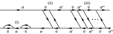
Figure 2: Diagrams for various tunneling processes: (i) quantum charge fluctuations, (ii) the co-tunneling process and (iii) the resonant tunneling process. The horizontal lines on the Keldysh contour represent the free propagators of the quantum dot. Remaining directed lines are tunneling lines.

II.3 Extension of resonant tunneling approximation

In order to account for the logarithmic behavior of Kondo correlations, we have to sum up a suitable class of diagrams of the expansion up to infinite order. The starting point of our approximation is the class of diagrams denoted as ‘resonant tunneling approximation’ (RTA) Konig1 . In the diagrammatic language, RTA includes all diagrams where any auxiliary vertical line cuts at most two tunneling lines [An example is presented in Fig. 2(iii)]. At not too low temperatures RTA was shown to provide a qualitatively reasonable approximation for the Kondo correlations with analytical expressions for the nonlinear differential conductance for arbitrary level degeneracy. It predicts also qualitatively reasonable behavior in the presence of Zeeman splitting. However, the original RTA developed in Ref. Konig1 does not describe the spin splitting since, as we will discuss below, it does not take into account the subclass of diagrams which accounts for spin-dependent quantum charge fluctuations.

To find the origin of the shortcoming, let us examine the QD spin dynamics. In general, in order to describe the superposition of spin states $|\!\uparrow\rangle$ and $|\!\downarrow\rangle$, it is necessary to consider also off-diagonal components of the density matrix in spin space, e.g., $P^{\sigma}_{\bar{\sigma}}$, where $\bar{\sigma}$ is the opposite spin of $\sigma$. The time evolution of $P^{\sigma}_{\bar{\sigma}}$ between time $t_{i}$ and $t$ ($t>t_{i}$) is described by the reduced propagator

$$\pi^{\sigma,\sigma}_{\bar{\sigma},\bar{\sigma}}(t,t_{i})\!=\!-i\langle\bar{\sigma}|{\rm Tr}_{L}{\rm Tr}_{R}\left[\rho^{L}_{0}\rho^{R}_{0}\,T_{C}\,S_{C}X_{\bar{\sigma}\,\sigma}(t)_{I}\right]|\sigma\rangle.$$ (14)

Since the tunneling Hamiltonian Eq. (5) conserves the spin, spin is conserved at each vertex. E.g., the spin indices of an incoming/outgoing tunneling line and an outgoing/incoming free propagator for each vertex are the same. Therefore, after Fourier transformation, Eq. (14) can be expressed as a Dyson equation,

$$\pi^{\sigma,\sigma}_{\bar{\sigma},\bar{\sigma}}(\omega)=1/(\omega+i0^{+}-\epsilon_{\sigma}+\epsilon_{\bar{\sigma}}-\sigma^{\sigma,\sigma}_{\bar{\sigma},\bar{\sigma}}(\omega)),$$ (15)

where $\sigma^{\sigma,\sigma}_{\bar{\sigma},\bar{\sigma}}$ denotes an irreducible self-energy and $0^{+}$ is a positive infinitesimal number. The diagrammatic representation of Eq. (15) is given in Fig. 3(a). Directed dotted lines carrying the energy $\omega$ correspond to the factor $\exp(i\omega t)$ of the Fourier transformation. The diagrams for $\sigma^{\sigma,\sigma}_{\bar{\sigma},\bar{\sigma}}$ are shown in Fig. 3(b), in which any auxiliary vertical line cuts at least one tunneling line.

Now, we observe that within RTA in any diagram for the self-energy of the master equation Eq. (12) a sector, where the reduced propagator $\pi^{\sigma,\sigma}_{\bar{\sigma},\bar{\sigma}}$ appears, is always accompanied by two tunneling lines, a left-going tunneling line with spin $\sigma$ and a right-going tunneling line with spin $\bar{\sigma}$, which are disconnected from $\pi^{\sigma,\sigma}_{\bar{\sigma},\bar{\sigma}}$ itself. It is a consequence of the requirement that any auxiliary vertical line must cut the same number of left- and right-going tunneling lines or free propagators with the same spin indices. This in turn follows from the fact that the spin is conserved at each vertex, and that the initial QD density matrix is assumed to be diagonal. As a result, the irreducible self-energy $\sigma^{\sigma,\sigma}_{\bar{\sigma},\bar{\sigma}}$ does not appear in RTA Konig1 , because in its presence, any auxiliary vertical line laying on a sector of $\sigma^{\sigma,\sigma}_{\bar{\sigma},\bar{\sigma}}$ would cut at least three tunneling lines. RTA can account for the Zeeman splitting of the Kondo resonance, which is already included in a denominator of the bare reduced propagator $\pi^{\sigma,\sigma}_{\bar{\sigma},\bar{\sigma}}$. However, RTA omits further information on the spin dynamics. As we will discuss in the following, the further information, such as the spin splitting $\Delta\epsilon$ caused by spin-dependent quantum charge fluctuations, is included in $\sigma^{\sigma,\sigma}_{\bar{\sigma},\bar{\sigma}}$ beyond the original RTA.

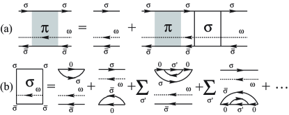
Figure 3: (a) Dyson equation for $\pi^{\sigma,\sigma}_{\bar{\sigma},\bar{\sigma}}$ and (b) the diagrammatic expansion of the irreducible self-energy $\sigma^{\sigma,\sigma}_{\bar{\sigma},\bar{\sigma}}$. Directed dotted lines carry the energy $\omega$.

In order to obtain an expression for $\sigma^{\sigma,\sigma}_{\bar{\sigma},\bar{\sigma}}$ we proceed in a perturbative expansion in terms of the coupling $\Gamma$,

$$\sigma^{\sigma,\sigma}_{\bar{\sigma},\bar{\sigma}}={\sigma^{\sigma,\sigma}_{\bar{\sigma},\bar{\sigma}}}^{(1)}+{\sigma^{\sigma,\sigma}_{\bar{\sigma},\bar{\sigma}}}^{(2)}+\cdots\;.$$ (16)

In lowest order we find the first two diagrams in the right-hand side of Fig. 3(b) describing spin-dependent quantum charge fluctuations. From them we obtain the first-order term

$${\sigma^{\sigma,\sigma}_{\bar{\sigma},\bar{\sigma}}}^{(1)}(\omega)\!\! = \!\!\int\!d\omega^{\prime}\frac{\gamma^{-}_{\sigma}(\omega^{\prime})}{\omega+i0^{+}-\omega^{\prime}+\epsilon_{\bar{\sigma}}}$$ (17)

$$+ \!\!\int\!d\omega^{\prime}\frac{\gamma^{-}_{\bar{\sigma}}(\omega^{\prime})}{\omega+i0^{+}+\omega^{\prime}-\epsilon_{\sigma}}$$

$$= \!\tilde{\gamma}^{-}_{\sigma}(\omega+\epsilon_{\bar{\sigma}})-\tilde{\gamma}^{-}_{\bar{\sigma}}(\epsilon_{\sigma}-\omega)^{*},$$

where $\gamma^{\pm}_{\sigma}\!=\!\sum_{r}\gamma^{\pm}_{r\sigma}$ and $\tilde{\gamma}^{\pm}_{\sigma}\!=\!\sum_{r}\tilde{\gamma}^{\pm}_{r\sigma}$. Here we introduced $\tilde{\gamma}^{\pm}_{r\sigma}$, which is the Hilbert transform of $\gamma^{\pm}_{r\sigma}$,

$$\!\!\!\!\!\!\!\!\!\tilde{\gamma}^{\pm}_{r\sigma}(\omega)=\int\!d\omega^{\prime}\frac{\gamma^{\pm}_{r\sigma}(\omega^{\prime})}{\omega+i0^{+}-\omega^{\prime}}$$ (18)

$$= \frac{\Gamma_{r\sigma}}{2\pi}\,\rho(\omega-\mu_{r})\biggl{\{}\pm\psi\!\left(\frac{1}{2}+\frac{D}{2\pi T}\right)$$

$$\mp \!{\rm Re}\,\psi\!\left(\frac{1}{2}+i\frac{\omega-\mu_{r}}{2\pi T}\right)+\pi\frac{\omega-\mu_{r}}{2D}\biggl{\}}-i\pi\gamma^{\pm}_{r\sigma}(\omega)\;,\;\;\;\;\;$$

and $\psi(x)$ denotes the digamma function. One can expect that the lowest order is sufficient for the description of the spin splitting. Indeed, for $E_{\rm Z}\!=\!T\!=\!eV\!=\!0$ and ferromagnetic leads ($P_{L}\!=\!P_{R}\!=\!P\!>\!0$), the spin splitting $\Delta\epsilon$ obtained by the scaling theory [Eq. (1)] is reproduced, ${\sigma^{\uparrow,\uparrow}_{\downarrow,\downarrow}}^{(1)}(\omega)\!\approx\!\Delta\epsilon$ for $|\omega/\epsilon_{0}|\!\ll\!1$. We further note that the self-energy given by Eq. (17) also describes the reduction of the Kondo resonance splitting below the value of the Zeeman energy $E_{\rm Z}$ for normal (nonmagnetic) leads. For $P_{L}\!=\!P_{R}\!=\!0$ and $T\!=\!eV\!=\!0$, the self-energy then reads,

$${\sigma^{\uparrow,\uparrow}_{\downarrow,\downarrow}}^{(1)}(\omega)\approx-\frac{\Gamma}{\pi}\tanh^{-1}\left(\frac{E_{\rm Z}}{-2\epsilon_{0}}\right),\;\Gamma\!=\!\sum_{\sigma,r}\frac{\Gamma_{r\sigma}}{2},$$ (19)

for $\epsilon_{\sigma}\!<\!0$ and $|\omega/\epsilon_{\sigma}|\ll 1$, which renormalizes and reduces $E_{Z}$. Such a reduction was derived before for the Anderson Moore and Kondo Rosch models.

Next, we discuss the nature and details of the extended RTA. The extension amounts to inserting into all possible positions in the diagrams of the original RTA expansion the lowest-order irreducible self-energy ${\sigma^{\sigma,\sigma}_{\bar{\sigma},\bar{\sigma}}}^{(1)}$ given by Eq. (17). The reduced propagator describing the time evolution of $P^{\sigma}_{0}$ is given by Eq. (14) with the replacement of $\bar{\sigma}$ by $0$:

$$\pi^{\sigma,\sigma}_{0,0}(\omega)=1/(\omega+i0^{+}-\epsilon_{\sigma}-\sigma^{\sigma,\sigma}_{0,0}(\omega))\;.$$ (20)

The resulting self-energy of the reduced propagator is represented by the diagrams from Fig. 4(a). It yields

$$\sigma^{\sigma,\sigma}_{0,0}(\omega)=\sum_{s=\pm}\int\!d\omega^{\prime}\frac{\gamma^{s}_{\sigma}(\omega^{\prime})}{\omega+i0^{+}-\omega^{\prime}}$$

$$+\int\!\!d\omega^{\prime}\gamma^{+}_{\bar{\sigma}}(\omega^{\prime})\,{\pi^{\sigma,\sigma}_{\bar{\sigma},\bar{\sigma}}}^{(1)}(\omega-\omega^{\prime})\;.$$ (21)

Here ${\pi^{\sigma,\sigma}_{\bar{\sigma},\bar{\sigma}}}^{(1)}$ is defined by Eq. (15) with the self-energy given by Eq. (17). The result is similar to the self-energy of the Green function obtained previously using EOM (Eq. (8) in Ref. Martinek1 ). The first term of Eq. (21) is related with spin $\sigma$ [the first and the second diagrams in the right-hand side of Fig. 4(a)]. The real part of this term causes a slight shift of the QD-level and the imaginary part gives a level broadening. The second term [the third diagram in the right-hand side of Fig. 4(a)] is associated with the Fermi distribution function of the opposite spin $\bar{\sigma}$ through $\gamma^{+}_{\bar{\sigma}}$ and is roughly proportional to $\int d\omega f^{+}(\omega)/(\omega\!+\!i0^{+}\mp E_{Z}\mp\Delta\epsilon)$ for $\sigma\!=\uparrow\!\!/\!\!\downarrow$ at $eV\!=\!0$. Consequently, the second term leads to the logarithmic behavior of Kondo correlations. Our result for $\sigma^{\sigma,\sigma}_{\bar{\sigma},\bar{\sigma}}$ provides a microscopic justification to lowest-order expansion in terms of $\Gamma$ for the spin splitting $\sigma\Delta\tilde{\epsilon}$ postulated in the EOM scheme (Eq. (9) of Ref. Martinek1 ).

The self-energy of the master equation (12) is given by

$$\Sigma_{\chi,\sigma}\! = \!-2i\,{\rm Im}\!\int d\omega\,\sum_{s=\pm}{\Lambda^{s}}^{\chi,\sigma}_{\chi,0}(\omega)\gamma^{s}_{\sigma}(\omega)\;,$$ (22)

and $\Sigma_{\chi,0}\!=\!-\!\sum_{\sigma=\uparrow,\downarrow}\Sigma_{\chi,\sigma}$ ($\chi\!=\!0,\uparrow,\downarrow$). The vertex functions $\Lambda^{+}$ and $\Lambda^{-}$ are determined by solving the diagrammatic equations depicted in Fig. 4(b). In the diagram for $\Lambda^{+/-}$, an open line carrying energy $\omega$ (dotted line) connects to the upper/lower horizontal line note2 . The diagrammatic equations can generate diagrams for the resonant tunneling processes in a recursive manner. The explicit forms are

$${\Lambda^{+}}^{\chi,\sigma}_{\chi,0}(\omega)\!\! = \!\!\pi^{\sigma,\sigma}_{0,0}(\omega)\,\biggl{\{}\delta_{\chi,0}-\int d\omega^{\prime}\sum_{s=\pm}\frac{{\Lambda^{s}}^{\chi,\sigma}_{\chi,0}(\omega^{\prime})^{*}\gamma^{s}_{\sigma}(\omega^{\prime})}{\omega+i0^{+}-\omega^{\prime}}$$

$$- \!\!\int d\omega^{\prime}\sum_{s=\pm}{\Lambda^{s}}^{\chi,\bar{\sigma}}_{\chi,0}(\omega^{\prime})^{*}\gamma^{s}_{\bar{\sigma}}(\omega^{\prime}){\pi^{\sigma,\sigma}_{\bar{\sigma},\bar{\sigma}}}^{(1)}(\omega-\omega^{\prime})\biggl{\}},$$

$${\Lambda^{-}}^{\chi,\sigma}_{\chi,0}(\omega)\!\! = \!\!\pi^{\sigma,\sigma}_{0,0}(\omega)$$ (24)

$$\times \!\!\biggl{\{}-\delta_{\chi,\sigma}-\int\!d\omega^{\prime}\sum_{s=\pm}\frac{{\Lambda^{s}}^{\chi,\sigma}_{\chi,0}(\omega^{\prime})^{*}\gamma^{s}_{\sigma}(\omega^{\prime})}{\omega+i0^{+}-\omega^{\prime}}\biggl{\}}.$$

Again in the right-hand side of Eq. (LABEL:eqn:vertex+), we inserted the self-energy ${\sigma^{\sigma,\sigma}_{\bar{\sigma},\bar{\sigma}}}^{(1)}$ via ${\pi^{\sigma,\sigma}_{\bar{\sigma},\bar{\sigma}}}^{(1)}$.

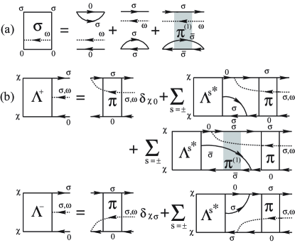
Figure 4: (a) The irreducible self-energy of the reduced propagator $\pi^{\sigma,\sigma}_{0,0}$. (b) Diagrammatic equations for the vertex functions ${\Lambda^{+}}^{\chi,\sigma}_{\chi,0}$ and ${\Lambda^{-}}^{\chi,\sigma}_{\chi,0}$. An open dotted line connects to the upper/lower horizontal line for $\Lambda^{\pm}$. Shaded boxes represent the off-diagonal component of the reduced propagator in the spin space ${\pi^{\sigma,\sigma}_{\bar{\sigma},\bar{\sigma}}}^{(1)}$.

From $P^{\rm st}_{\sigma}$, which is obtained by solving the master equation Eq. (12), we find the average occupation $N$ and the local magnetization $M$ of the QD,

$$N=P^{\rm st}_{\uparrow}+P^{\rm st}_{\downarrow}\;,\;\;M=(1/2)(P^{\rm st}_{\uparrow}-P^{\rm st}_{\downarrow})\;.$$ (25)

The spin-dependent nonequilibrium DOS of the QD is defined as

$$\rho_{\sigma}(\omega)\!=\!-\frac{1}{2i\pi}\{G^{>}_{\sigma}(\omega)-G^{<}_{\sigma}(\omega)\},$$ (26)

where the lesser/greater Green functions are expressed, using Eqs. (LABEL:eqn:vertex+) and (24), as

$$G^{\gtrless}_{\sigma}(\omega)=2i\,{\rm Im}\!\!\!\sum_{\chi=0,\uparrow,\downarrow}P^{\rm st}_{\chi}{\Lambda^{\pm}}^{\chi,\sigma}_{\chi,0}(\omega).$$ (27)

Also the transport current flowing into the QD through the junction $r$, $I_{r}$, can be expressed in terms of the Green functions. The spin-resolved components read

$$I_{r\sigma}=-ie\int\!d\omega\,\{\gamma_{r\sigma}^{+}(\omega)\,G^{>}_{\sigma}(\omega)+\gamma_{r\sigma}^{-}(\omega)\,G^{<}_{\sigma}(\omega)\}.$$ (28)

One can prove that the approximation satisfies spin and charge conservation note4 . Equations (22), (27) and (28) combine to $\sum_{r}I_{r\sigma}\!=\!ie\sum_{\chi}P^{st}_{\chi}\,\Sigma_{\chi,\sigma}$, which by virtue of the master equation, Eq. (12) leads to the spin-resolved current conservation, $\sum_{r}I_{r\sigma}\!=\!0$. The conservation laws for charge and spin,

$$I_{L}\!=\!-I_{R}\!=\!I,\;\;\;\sum_{r}(I_{r\uparrow}-I_{r\downarrow})\!=\!0,$$ (29)

follows the spin-resolved current conservation. Equation (29) is valid only for collinear magnetizations, where the spin is conserved at each vertex in the diagrams of the self-energy for the master equation, regardless of the sign of $P_{L(R)}$. This fact ensures that the self-energy of master equation does not mix diagonal and off-diagonal states and allows one to formulate a closed equation for the diagonal components of the reduced density matrix.

The linear conductance, $G_{\sigma}^{\rm lin}\!\equiv\!\lim_{V\rightarrow 0}dI_{\sigma}(V)/dV$ [$I_{\sigma}\!=\!I_{r\sigma}$], probes the equilibrium spin-dependent DOS, $\rho_{\sigma}^{eq}(\omega)$, around the Fermi energy:

$$\frac{G_{\sigma}^{\rm lin}}{G_{\rm K}}=2\pi\frac{\Gamma_{L\sigma}\Gamma_{R\sigma}}{\Gamma_{L\sigma}\!+\!\Gamma_{R\sigma}}\int\!d\omega\,\biggl{\{}-\frac{\partial f^{+}(\omega)}{\partial\omega}\biggl{\}}\,\rho_{\sigma}^{eq}(\omega),$$ (30)

where $G_{\rm K}\equiv e^{2}/(2\pi\hbar)$ is the conductance quantum. We symmetrized the expression Eq. (30) using the spin and charge conservation, Eq. (29).

III Results and discussions

In this section, we will present results obtained by solving the integral equations numerically. In all results we tested the numerical accuracy by checking the spin and charge conservation ( the relative error is smaller than $5\!\times\!10^{-6}$). We also checked the spectral sum rule, $\int d\omega\,\rho_{\sigma}(\omega)\!=\!P^{\rm st}_{0}+P^{\rm st}_{\sigma}$, which follows from the fact that ${\Lambda^{\pm}}^{\chi,\sigma}_{\chi,0}(\omega)$ is analytic in the upper half plane and decays at infinity as $1/\omega$. The sum rule is always satisfied with accuracy better than $5\!\times\!10^{-4}$.

In Sec. III.1, we will discuss the splitting of the zero-bias anomaly. Subsections III.2 and III.3 provide a discussion of the restoration of the Kondo resonance as well as of properties of the nonequilibrium Kondo effect. In theses subsections, we will assume a left-right symmetry in the coupling strengths $\Gamma_{L}\!=\!\Gamma_{R}$ [$\Gamma_{r}\!\equiv\!(\Gamma_{r\uparrow}+\Gamma_{r\downarrow})/2$] and spin polarization factors $P_{L}\!=\!|P_{R}|$, and $a_{c}\!=\!0$. In equilibrium these symmetries are not important because, as one can see from a unitary transformation Martinek2 , an asymmetry gives just a constant prefactor to the linear conductance. However, this is not the case for a nonequilibrium state, as will be shown in Sec. III.4.

III.1 Splitting of the zero bias anomaly

Figure 5(a) shows the nonlinear differential conductance $G_{\rm P}(V)\!\equiv\!dI(V)/dV$ for P alignment and symmetric coupling, $\Gamma_{L}\!=\!\Gamma_{R}$, and spin polarization, $P_{L}\!=\!P_{R}$. The splitting of the zero-bias anomaly is well observable for low temperatures. The enhancement of the peak at low temperatures is a clear sign of Kondo correlations. The value of the splitting is independent of temperature and almost coincides with the prediction of the scaling theory Eq. (1), $2\Delta\epsilon\!\approx\!0.204\Gamma$. At high temperature, the two peaks are smeared out. However, the magnitude of the splitting is not affected by the temperature.

Figure 5(b) shows the corresponding plot for the local magnetization $M$. For small bias voltage $|eV|\lesssim|\Delta\epsilon|$, it increases with decreasing temperature. At the same time, the differential conductance decreases [Fig. 5(a)]. This indicates that the suppression of the zero-bias anomaly can be attributed to the quenching of the spin-flip scattering at low temperatures. When the applied bias voltage exceeds the spin-splitting energy, $|eV|\gtrsim|\Delta\epsilon|$, a spin-flip channel opens. As a result, the local magnetization starts to decrease and peaks appear in the nonlinear differential conductance.

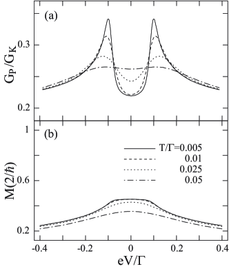
Figure 5: (a) The nonlinear differential conductance and (b) the local magnetization $M$ for the P alignment ($P_{L}\!=P_{R}\!=\!0.1$) and for symmetric coupling $\Gamma_{L}\!=\!\Gamma_{R}$. Solid, dashed, dotted and dot-dashed lines are results for various temperatures $T/\Gamma=0.005,0.01,0.025$, and $0.05$, respectively. Parameters are: $\epsilon_{0}/\Gamma\!=\!-2$, $D/\Gamma\!=\!50$.

III.2 Restoration of Kondo resonance

A remarkable feature of the spin splitting induced by ferromagnetism is that it can be compensated by an applied magnetic field Martinek1 ; Martinek2 . At the point of full compensation, the strong coupling limit can be retrieved. The Kondo temperature in the leading logarithmic approximation is given by Martinek1

$$T_{\rm K}(P)\approx\tilde{\epsilon}\,\exp\biggl{\{}\frac{-\pi\tilde{\epsilon}}{\Gamma}\,\frac{\arctan(P)}{P}\biggl{\}}\;.$$ (31)

Here we considered the case $P_{L}\!=\!P_{R}\!=\!P$. The ratio $\Gamma/(\pi\tilde{\epsilon})$ corresponds the value $J_{0}(\nu_{\uparrow}+\nu_{\downarrow})$ of Ref. Martinek1 . The cutoff energy $\tilde{\epsilon}$ follows from $\tilde{\epsilon}\!=\!-\epsilon_{0}\!+\!\Gamma/(2\pi)\ln(\tilde{\epsilon}/D)$.

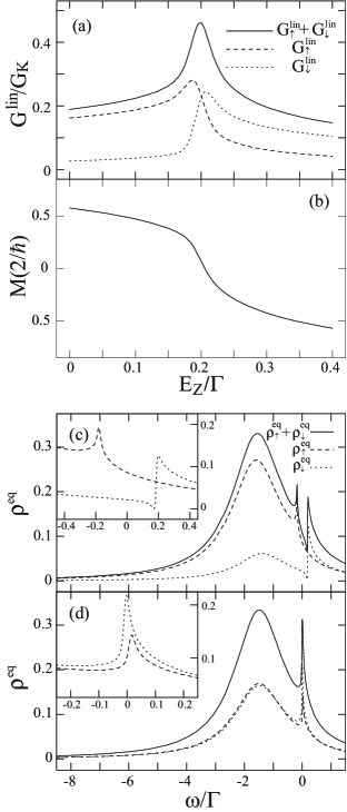
Figure 6: (a) The linear conductance $G^{\rm lin}$ and the local magnetization $M$ as a function of the Zeeman energy $E_{\rm Z}$ for the P alignment ($P_{L}\!=\!P_{R}\!=\!0.2$). In panel (a), the spin-resolved conductance is plotted by dashed (dotted) line for up (down) spin. The equilibrium DOS for (c) $E_{\rm Z}/\Gamma\!=\!0$ and (d) $E_{\rm Z}/\Gamma\!=0.205$. Solid and dashed (dotted) lines show the total DOS and the spin resolved DOS for up (down) spin. Insets in these panels are blow-ups of the Kondo resonance. Parameters are: $T/\Gamma\!=\!0.005$, $\epsilon_{0}/\Gamma\!=\!-2$, $D/\Gamma\!=\!50$.

Figure 6(a) and (b) show the linear conductance $G^{\rm lin}$ and the local magnetization $M$ as a function of Zeeman energy $E_{\rm Z}$ in equilibrium for the parallel alignment. The average occupation $N$ depends slightly on $E_{\rm Z}$ and varies between $N\!\approx\!0.88$ and $N\!\approx\!0.91$. At $E_{\rm Z}\!=\!0$, the direction of the local magnetization $M$ and lead magnetizations are aligned. With increasing Zeeman energy the local magnetization $M$ changes the direction. At a peak in the linear conductance $G^{\rm lin}$, where spin-flip processes are expected to be enhanced [solid line in Fig. 6(a)], we observe the local magnetization $M\!=\!0$ in agreement with results from Ref. Martinek2 . The spin state of the QD is responsible for the slight asymmetry in the conductance around the $M\!=\!0$ point. In the left (right) side of the peak, because the QD level is occupied by an up-spin (down-spin) electron, the co-tunneling current for up-spin (down-spin) component is dominant [dashed (dotted) line in Fig. 6(a)]. As the up-spins are majority spins, a larger conductance is obtained on the left side of the peak.

We analyzed the DOS at $E_{\rm Z}\!=\!0$ [Fig. 6(c)] and at $E_{\rm Z}\!=\!0.205\,\Gamma$, where $M\!\approx\!0$ [Fig. 6(d)]. The solid and dashed (dotted) lines show the total DOS $\rho(\omega)\equiv\sum_{\sigma}\rho_{\sigma}(\omega)$ and the up-spin (down-spin) component of the DOS $\rho_{\sigma}(\omega)$, respectively. Figure 6(c) and its inset demonstrate that the Kondo resonance splits at $E_{\rm Z}\!=\!0$. The two resonances, which appear rather well resolved, should be smeared by decoherence effects. These effects are beyond the present approximation, as we will discuss in Sec. IV. The enhancement/suppression of the up/down spin (dashed/dotted line) component of the QD-level DOS (broad peak around $\omega/\Gamma\!=\!-2$) indicates the positive local magnetization, $M\!>\!0$.

At $E_{\rm Z}\!=\!0.205\,\Gamma$, the Kondo resonance is restored at the Fermi energy [solid line in Fig. 6(d)]. We can observe that the resonance for the minority-spin component (dotted line) is higher than that of the the majority-spin component (dashed line) [inset in Fig. 6(d)]. Loosely speaking, it is because the minority (majority) spin in the QD is well (poorly) screened by majority (minority) spin in leads. This tendency is consistent with the zero-temperature result of NRG Martinek2 and the Friedel sum rule, which predicts $\rho_{\sigma}(0)\sim 1/\Gamma_{\sigma}$ Martinek2 .

As for the QD-level DOS, up-spin and down-spin components are almost the same (at $E_{\rm Z}\!=\!0.205\,\Gamma$), which indicates $M\!=\!0$ [dotted and dashed lines in Figs. 6(d)]. However, though the QD level can be spin polarized depending on $E_{Z}$, the total QD-level DOS is not affected by $E_{Z}$, i.e. the solid lines in Figs. 6(c) and (d) can almost overlap around the broad peak. Such a feature is also obtained from the NRG work MSChoi .

III.3 Kondo resonance out of equilibrium

In this subsection, we will discuss the nonequilibrium Kondo effect. Fig. 7 shows the nonlinear differential conductance, $G$ [(a) and (c)], and the local magnetization, $M$ [(b) and (d)], for symmetric coupling. As discussed in Sec. III.1, we can observe the splitting of the zero-bias anomaly for parallel alignment [solid line in (a)]. However, for antiparallel alignment [solid line in (c)], the splitting vanishes. Moreover, for positive (negative) bias voltage spin accumulates in the QD with positive (negative) local magnetization [solid line in (d)].

As discussed in Sec. III.2, the zero-bias anomaly is expected to be restored when the spin splitting is compensated by an applied magnetic field. The dashed line in (c) shows the case for the P alignment with $E_{\rm Z}\!=\!0.205\,\Gamma$. Figures 7 (e) and (f) show the nonequilibrium DOS $\rho_{\sigma}(\omega)$ for the AP alignment and that for the P alignment with the Zeeman energy $E_{\rm Z}\!=\!0.205\,\Gamma$. The total DOS has two peaks (solid lines) at two chemical potentials, similar in shape to that of a nonequilibrium Kondo DOS split by an applied voltage. However, now the two peaks are spin polarized, i.e. there is clear difference in the weights for the spin-up component $\rho_{\uparrow}(\omega)$ (dashed lines) and the spin-down component $\rho_{\downarrow}(\omega)$ (dot-dashed lines).

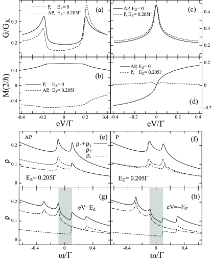
Figure 7: The nonlinear differential conductance $G$, (a) and (c), and the local magnetization $M$, (b) and (d), for a symmetric coupling $\Gamma_{L}\!=\!\Gamma_{R}$. Solid lines and dashed lines in (a) and (c) are plots for $E_{\rm Z}\!=\!0$ and $E_{\rm Z}\!=\!0.205\,\Gamma$, respectively. The solid lines in (a) and (c) are for the P alignment ($P_{L}\!=\!P_{R}\!=\!0.2$) and the AP alignment ($P_{L}\!=\!-P_{R}\!=\!0.2$)], respectively. The dashed lines in (a) and (c) are for the AP alignment and the P alignment, respectively. The average occupation is $N\!\approx\!0.89$ for all parameter regimes. The panels (e) and (f) show the corresponding DOS $\rho(\omega)$ of the solid and the dashed lines in panel (c) at $eV/\Gamma\!=\!0.205$. The dashed and dot-dashed lines are for $\rho_{\uparrow}(\omega)$ and $\rho_{\downarrow}(\omega)$, respectively. Panels (g) and (h) show plots of the DOS $\rho(\omega)$ of the dashed line in panel (a) at $eV\!=\!E_{\rm Z}$ (g), and at $eV\!=\!-E_{\rm Z}$ (h). The other parameters are the same as for Fig. 6.

For the AP alignment with the Zeeman energy $E_{\rm Z}\!=\!0.205\,\Gamma$, the splitting persists [dashed line in (a)], but in this case the splitting is caused by the Zeeman energy Meir1 , and a strong asymmetry between two peaks is obtained. Intuitively, the result can be understood by the following argument: In the regime $|eV|\!\lesssim\!E_{\rm Z}$, a spin-down occupies the QD level. Above a positive bias voltage $eV\!\geq\!E_{\rm Z}$, spin-flip tunneling events from a left lead spin-up state to a right lead spin-down state contribute to the current. In this case, because both initial and final states are majority-spin states, a large peak is expected. On the other hand, at negative bias voltages $eV\!\leq\!-E_{\rm Z}$, the spin-flip tunneling processes are between minority spin states. Hence the peak in the differential conductance is weak.

A more precise explanation taking into account Kondo correlations can be given based on the spin-polarized nonequilibrium Kondo resonance. Figure 7(g) shows $\rho(\omega)$ for $eV\!=\!E_{\rm Z}\!=\!0.205\,\Gamma$. The two spin polarized Kondo resonances out of equilibrium split further into four peaks (solid line) by the energy $eV$ Meir1 . The lower two peaks at $-E_{\rm Z}+eV/2$ and $-E_{\rm Z}-eV/2$ are for spin-down (dot-dashed line), related to the left and right lead chemical potential at $\pm eV/2$, respectively. The peak at $-E_{\rm Z}+eV/2$ is larger than the peak at $-E_{\rm Z}-eV/2$, because the spin-down electron in the QD can be screened by majority spins of the left lead with spin-up. The peaks at $E_{\rm Z}\pm eV/2$ are for spin-up electrons (dashed line), and a larger amplitude of the peak at $E_{\rm Z}-eV/2$ can be explained in the same way as above. Under the condition $eV\!=\!E_{\rm Z}$, the positions of the two large peaks at $E_{\rm Z}-eV/2$ and $-E_{\rm Z}+eV/2$ coincide with the two chemical potentials. Thus, tunneling electrons with energy between the left and right chemical potentials [shaded region in (g)] can profit from the larger DOS inside the QD. Consequently, the differential conductance $G_{\rm AP}(V)$ at positive bias voltage $eV=E_{\rm Z}$ is enhanced more strongly. Finally, Fig. 7(h) shows the DOS $\rho(\omega)$ for $eV\!=\!-E_{\rm Z}\!=\!-0.205\,\Gamma$. By repeating the same arguments as presented above, we can explain the fact that at negative bias voltage $eV=-E_{\rm Z}$ the DOS $\rho(\omega)$ of the QD at energies between the left and right Fermi levels [shaded region in (h)] is lower, and consequently the peak of the differential conductance $G_{\rm AP}(V)$ is smaller as well.

The anomalous behavior of the nonlinear conductance determines the shape of the TMR. Figure 8 presents the TMR defined as

$${\rm TMR}\equiv(G_{\rm P}(V)-G_{\rm AP}(V))/G_{\rm AP}(V).$$ (32)

We find a large negative TMR at zero bias. This is in contrast to the TMR of ferromagnetic tunnel junctions, where one finds usually a maximum of the TMR at zero bias and then a decrease with increasing bias voltage $V$ Maekawabook ; Utsumi1 .

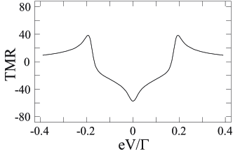
Figure 8: The tunnel magnetoresistance TMR as function of the bias voltage $V$. Spin polarization factors are $P_{L}\!=\!|P_{R}|\!=\!0.2$. The further parameters are the same as for Fig. 6.

III.4 Left-right asymmetry in system parameters

In the previous subsection we showed that the spin-polarization of the Kondo resonance and the spin-accumulation for a nonequilibrium situation depend on the orientation of the lead magnetizations. We can expect that a left-right asymmetry in coupling strengths, $\Gamma_{R}\!\neq\!\Gamma_{L}$, and spin polarization, $P_{R}\!\neq\!P_{L}$, or an asymmetry in the applied voltage could affect these properties as well and leave footprints on the nonlinear differential conductance. In the following we discuss several examples.

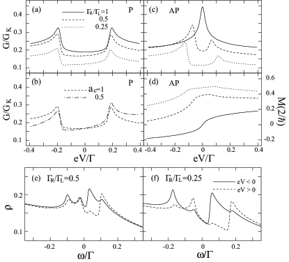
Figure 9: (a) The differential conductance for the P alignment $G_{\rm P}(V)$ ($P_{L}\!=P_{R}\!=\!0.2$). Solid lines, dashed lines and dotted lines are results for $\Gamma_{R}/\Gamma_{L}\!=\!1,0.5$, and $0.25$. (b) The differential conductance $G_{\rm P}(V)$ for $\Gamma_{R}/\Gamma_{L}\!=\!0.5$ with the asymmetry factor $a_{c}\!=\!0$ (dashed line) and $0.5$ (dot-dashed line). (c) The differential conductance with the AP alignment $G_{\rm AP}(V)$ ($P_{L}\!=-P_{R}\!=\!0.2$) and (d) the nonequilibrium local magnetization $M$. (e), (f) The total DOS $\rho(\omega)$ in the AP alignment: (e) The solid (dashed) line is for $\Gamma_{R}/\Gamma_{L}\!=\!0.5$ at $eV/\Gamma\!=\!-0.08$ ($0.07$). (f) The solid (dashed) line is for $\Gamma_{R}/\Gamma_{L}\!=\!0.25$ at $eV/\Gamma\!=\!-0.13$ ($0.11$). The other parameters are the same as for Fig. 6.

Figure 9(a) shows the nonlinear differential conductance $G_{\rm P}(V)$ for the P alignment ($P_{L}\!=\!P_{R}\!=\!0.2$) for varying values of the ratio of coupling strengths $\Gamma_{R}/\Gamma_{L}$, while keeping the total coupling $\Gamma=\Gamma_{L}+\Gamma_{R}$ unchanged. The values of the splittings are almost the same for all cases. The reason is the following: The spin splitting Eq. (1) is expressed as the sum of the left and right contributions $\Delta\epsilon\equiv\Delta\epsilon_{L}+\Delta\epsilon_{R}$ (one can obtain the relation for $\Delta\epsilon_{r}$ using Eq. (1) and adding a lead index $r$ to the $\Gamma$ and $P$). For $P_{L}\!=\!P_{R}\!=\!P$, the value of the splitting $\Delta\epsilon$ is proportional to $P(\Gamma_{L}+\Gamma_{R})$, which is independent of the ratio of coupling strength. The asymmetric capacitive coupling does not alter the conductance $G(V)$ by much. Figure 9(b) shows curves for the asymmetry factor $a_{c}\!=\!0$ (dashed line) and $0.5$ (dot-dashed line) for $\Gamma_{R}/\Gamma_{L}\!=\!0.5$ [the dashed line is the same as that in (a)]. The asymmetry factor just tilts the curve slightly.

Figure 9(c) presents the nonlinear conductance $G_{\rm AP}(V)$ for the AP alignment for different values of $\Gamma_{R}/\Gamma_{L}$, and $a_{c}\!=\!0$. For an asymmetric coupling, we find again a splitting of the zero bias anomaly. Such a splitting was observed experimentally Pasupathy (details are given in Sec. V). It can be understood because the spin splitting due to the exchange interaction with the left $\Delta\epsilon_{L}$ and right lead $\Delta\epsilon_{R}$ cannot compensate each other $\Delta\epsilon_{L}\neq-\Delta\epsilon_{R}$ for $\Gamma_{L}\!\neq\!\Gamma_{R}$. Actually, with decreasing $\Gamma_{R}/\Gamma_{L}$, $\Delta\epsilon$ increases and thus the splitting is enhanced.

We observe the asymmetry in the two peaks’ amplitude similar to the case of the AP alignment with the Zeeman splitting [dashed line in Fig. 7(a)]. Actually, this asymmetry can be explained almost in the same way. The only difference is that the large peak is at negative bias voltage [dashed and dotted lines in Fig. 9(c)] as opposed to the dashed line in Fig. 7(a), because, $\Delta\epsilon$ is negative whereas the Zeeman energy is positive. The solid (dashed) lines in panels (e) and (f) show the total DOS $\rho(\omega)$ for the AP alignment at negative (positive) bias voltage. We can check that the larger DOS at negative bias voltage (solid lines) is responsible for higher conductance peak.

Next, we will look at consequences of an asymmetry in left and right spin polarization factors $P_{L}\!\neq\!P_{R}$. The dashed and dotted lines in Fig. 10 show the differential conductance $G(V)$ (a) and local magnetization $M$ (b) for various spin polarization factors but for symmetric coupling strength $\Gamma_{R}=\Gamma_{L}$. For each curve, the average value of polarization factors in the left and right leads was kept constant $(P_{L}+P_{R})/2\!=\!0.1$. The solid lines show the result for the equal polarizations ($P_{L}\!=\!P_{R}\!=\!0.1$). As the spin polarization of the left lead increases ($P_{L}\!=\!0.4$ for dashed lines, $P_{L}\!=\!0.6$ for dotted lines) the local magnetization increases (decreases) for positive (negative) bias voltage [Fig. 10(b)] and accordingly, the difference between the two peaks grows [Fig. 10(a)]. The solid (dashed) lines in panels (c) and (d) are the total DOS at negative (positive) bias voltage [(c) for $P_{L}\!=\!0.4$ and (d) for $0.6$]. It confirms that with increasing $P_{L}$, the difference in the intensity increases, causing the large difference in peak heights.

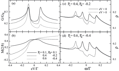
Figure 10: (a) The nonlinear conductance $G(V)$ and (b) the local magnetization $M$ for various spin polarizations ($P_{L}$, $P_{R}$) and for symmetric coupling $\Gamma_{R}\!=\!\Gamma_{L}$. The average value of the polarization factors in the left and right leads are fixed as $(P_{L}+P_{R})/2\!=\!0.1$. The solid, dashed, and dotted lines are for $P_{L}\!=\!0.1$, $0.4$, and $0.6$, respectively. The total DOS $\rho(\omega)$ at $eV/\Gamma\!=\!-0.1$ (solid line) and $eV/\Gamma\!=\!0.1$ (dashed line) for $P_{L}\!=\!0.4$ (c) and $P_{L}\!=\!0.6$ (d). The other parameters are the same as for Fig. 6.

IV Decoherence effect

In this section, we will turn our attention to the effects of decoherence. Since the transverse spin relaxation time, $T_{2}$, is defined as the decay time of the off-diagonal components of the reduced density matrix $P^{\sigma}_{\bar{\sigma}}$, one might identify it within the Markov approximation with the imaginary part of the corresponding off-diagonal component of the self-energy in Fourier space,

$$1/T_{2}=-{\rm Im}\,\sigma^{\sigma,\sigma}_{\bar{\sigma},\bar{\sigma}}(\epsilon_{\sigma}\!-\!\epsilon_{\bar{\sigma}}).$$ (33)

The relevant frequency in the argument $\epsilon_{\sigma}\!-\!\epsilon_{\bar{\sigma}}$ is the energy difference between the states with spin $\sigma$ and the opposite spin $\bar{\sigma}$. From Eq. (15), one can conclude, that $1/T_{2}$ is closely related to the broadening of Kondo resonance. When evaluating the self-energy we note that the lowest-order contribution to $\sigma^{\sigma,\sigma}_{\bar{\sigma},\bar{\sigma}}$ does not contain an imaginary part. In the following, we therefore, perform the second order perturbation expansion in terms of $\Gamma$ at zero temperature $T\!=\!0$ and $\epsilon_{r\sigma}\!\equiv\!\epsilon_{\sigma}-\mu_{r}<0$.

The first diagram of the second-order expansion, depicted in Fig. 3(b), is evaluated as

$${\sigma^{\sigma,\sigma}_{\bar{\sigma},\bar{\sigma}}}^{\text{(2-1)}}(\epsilon_{\sigma}\!-\!\epsilon_{\bar{\sigma}})=\sum_{\sigma^{\prime}}\int\!d\omega^{\prime}d\omega^{\prime\prime}\frac{1}{\epsilon_{\sigma}-\omega^{\prime}+i0^{+}}$$

$$\times\frac{\gamma^{+}_{\sigma^{\prime}}(\omega^{\prime\prime})\,\gamma^{-}_{\sigma}(\omega^{\prime})}{(\epsilon_{\sigma}-\epsilon_{\sigma^{\prime}}-\omega^{\prime}+\omega^{\prime\prime}+i0^{+})(\epsilon_{\sigma}-\omega^{\prime}+i0^{+})}.$$ (34)

For simplicity, we assume here a flat DOS with cutoff energy $D$, i.e., we replace the Lorentzian cutoff function by $\rho_{\rm c}(\omega)\rightarrow\theta(\omega+D)\theta(D-\omega)$ with $|\epsilon_{r\sigma}|\!\ll\!D$. Then, the imaginary part of Eq. (34) reads,

$$- \!{\rm Im}\,{\sigma^{\sigma,\sigma}_{\bar{\sigma},\bar{\sigma}}}^{\text{(2-1)}}(\epsilon_{\sigma}\!-\!\epsilon_{\bar{\sigma}})$$ (35)

$$\approx \!\!\!\!\!\sum_{\sigma^{\prime}rr^{\prime}}\pi\frac{\Gamma_{r\sigma}\Gamma_{r^{\prime}\sigma^{\prime}}}{(2\pi)^{2}}\frac{\epsilon_{r\sigma}-\epsilon_{r^{\prime}\sigma^{\prime}}}{\epsilon_{r\sigma}\,\epsilon_{r^{\prime}\sigma^{\prime}}}\,\theta(\epsilon_{r\sigma}-\epsilon_{r^{\prime}\sigma^{\prime}})\;.$$

The second diagram of the second-order expansion is obtained from Eq. (34) as ${\sigma^{\sigma,\sigma}_{\bar{\sigma},\bar{\sigma}}}^{\text{(2-2)}}(\omega)\!=\!-{\sigma^{\bar{\sigma},\bar{\sigma}}_{\sigma,\sigma}}^{\text{(2-1)}}(-\omega)^{*}$. In addition to the above two diagrams there are four other diagrams (Fig. 11); however their imaginary part vanishes for $\epsilon_{r\sigma}\!<\!0$:

$${\rm Im}\,{\sigma^{\sigma,\sigma}_{\bar{\sigma},\bar{\sigma}}}^{\text{(2-3)}}(\epsilon_{\sigma}\!-\!\epsilon_{\bar{\sigma}})=$$ (36)

$${\rm Im}\int\!d\omega^{\prime}d\omega^{\prime\prime}\frac{\gamma^{-}_{\bar{\sigma}}(\omega^{\prime})\,\gamma^{-}_{\sigma}(\omega^{\prime\prime})}{\omega^{\prime}-\omega^{\prime\prime}+\epsilon_{\sigma}-\epsilon_{\bar{\sigma}}+i0^{+}}$$

$$\times \biggl{(}\frac{1}{\omega^{\prime}-\epsilon_{\bar{\sigma}}+i0^{+}}+\frac{1}{\epsilon_{\sigma}-\omega^{\prime\prime}+i0^{+}}\biggl{)}^{2}$$

$$\approx \sum_{rr^{\prime}}\frac{\Gamma_{r\sigma}\,\Gamma_{r^{\prime}\bar{\sigma}}}{4\pi}\biggl{(}\frac{\theta(\epsilon_{r^{\prime}\bar{\sigma}})}{\epsilon_{r\sigma}}+\frac{\theta(\epsilon_{r\sigma})}{\epsilon_{r^{\prime}\bar{\sigma}}}\biggl{)}=0\;.$$

By adding the contributions from ${\sigma^{\sigma,\sigma}_{\bar{\sigma},\bar{\sigma}}}^{\text{(2-1)}}$ and ${\sigma^{\sigma,\sigma}_{\bar{\sigma},\bar{\sigma}}}^{\text{(2-2)}}$, one obtains the transverse spin relaxation rate in 2nd order,

$$\frac{1}{T_{2}^{(2)}}\approx\sum_{\sigma\sigma^{\prime}}\frac{\Gamma_{L\sigma}\Gamma_{R\sigma^{\prime}}\,|\epsilon_{L\sigma}-\epsilon_{R\sigma^{\prime}}|}{4\pi\,\epsilon_{L\sigma}\,\epsilon_{R\sigma^{\prime}}}\;.$$ (37)

The rate is proportional to the sum of spin flip and spin preserving co-tunneling currents. This result is consistent with $\sum_{\sigma}1/\tau_{\sigma}$ derived in Refs. Meir1 ; Meir2 ($\tau_{\sigma}$ is defined in Eq. (5) of Ref. Meir1 or Eq. (43) of Ref. Meir2 ), where the decoherence effect due to the dissipative current flow for finite bias and/or magnetic field even at zero temperature was first pointed out.

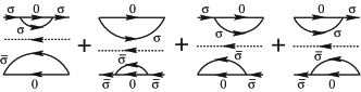
Figure 11: The four additional diagrams of second order expansion for the irreducible self-energy $\sigma^{\sigma,\sigma}_{\bar{\sigma},\bar{\sigma}}$. One bubble dresses each horizontal line. The other two diagrams, where one bubble is inside the other bubble are depicted in Fig. 3(b). Here, dashed lines carry the energy $\epsilon_{\sigma}-\epsilon_{\bar{\sigma}}$.

Because the RTA ignores $\sigma^{\sigma,\sigma}_{\bar{\sigma},\bar{\sigma}}$, it predicts sharp conductance peaks split by the magnetic field Konig1 . As stressed in Refs. Meir1 ; Rosch , we cannot neglect the decoherence effect, since it could provide the cutoff energy for Kondo correlations and thus suppresses the Kondo effect. In second order perturbation theory, discussed above, the decoherence effect appears to be weak, causing only slight changes of the DOS. However, a more thorough analysis reveals that second order perturbation theory is not enough: it does not account for Kondo correlations which also enhance the decoherence Rosch ; Paaske2 . In order to describe this enhancement, we have to sum up infinite order diagrams again.

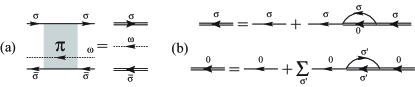
Figure 12: (a) The off-diagonal component of the reduced propagator in spin space within NCA. Double lines on the Keldysh contour are determined by Dyson equations in (b).

A convenient way to include diagrams up to the infinite order is provided by the NCA Kuramoto ; Bickers ; Hewson . The naive application of NCA causes a spurious peak at the Fermi energy (see Sec. I), but the NCA for the off-diagonal component of the reduced propagator in spin space $\pi^{\sigma,\sigma}_{\bar{\sigma},\bar{\sigma}}$ is free from this flaw as shown below. The diagram of $\pi^{\sigma,\sigma}_{\bar{\sigma},\bar{\sigma}}$ within NCA is depicted in Fig. 12(a). Double lines are ‘full’ propagators of the QD state and determined by Dyson equations generating the infinite numbers of ‘non-crossing’ diagrams [Fig. 12(b)]. We observe that diagrams in first and second order expansion of $\sigma^{\sigma,\sigma}_{\bar{\sigma},\bar{\sigma}}$ [Figs. 3(b) and  11] are contained in the NCA diagrams. The expression is given by

$$\pi^{\sigma,\sigma}_{\bar{\sigma},\bar{\sigma}}(\omega)=\int d\omega_{1}d\omega_{2}\frac{\rho_{\sigma}(\omega_{1})\,\rho_{\bar{\sigma}}(\omega_{2})}{\omega+i0^{+}-\omega_{1}+\omega_{2}},$$ (38)

where $\rho_{\chi}(\omega)$ is the spectral density of the full propagator of the QD state $|\chi\rangle$, obtained by the following self-consistent equations:

$$\rho_{\sigma}(\omega) = -\frac{1}{\pi}{\rm Im}\frac{1}{\omega+i0^{+}-\epsilon_{\sigma}-\Sigma_{\sigma}(\omega)},$$ (39)

$$\Sigma_{\sigma}(\omega) = \int d\omega^{\prime}\tilde{\gamma}^{-}_{\sigma}(\omega-\omega^{\prime})\rho_{0}(\omega^{\prime}),$$ (40)

$$\rho_{0}(\omega) = -\frac{1}{\pi}{\rm Im}\frac{1}{\omega+i0^{+}-\Sigma_{0}(\omega)},$$ (41)

$$\Sigma_{0}(\omega) = -\sum_{\sigma^{\prime}}\int d\omega^{\prime}\tilde{\gamma}^{+}_{\sigma^{\prime}}(\omega^{\prime}-\omega)^{*}\rho_{\sigma^{\prime}}(\omega^{\prime}).$$ (42)

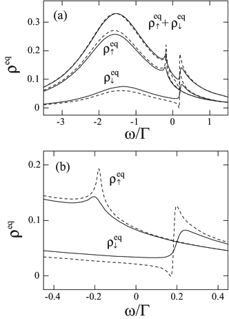
Figure 13: (a) The total and spin resolved DOS for parallel alignment ($P_{L}\!=\!P_{R}\!=\!0.2$) within NCA for $\pi^{\sigma,\sigma}_{\bar{\sigma},\bar{\sigma}}$ (solid lines). The panel (b) is the magnification around the Kondo resonance. Dotted lines are the results without decoherence effect and correspond to lines in Fig. 6(c). Parameters are the same as those in Fig. 6.

Figures 13(a) and (b) show the total and spin resolved DOS and their magnifications for parallel alignment ($P_{L}\!=\!P_{R}\!=\!0.2$) within NCA for $\pi^{\sigma,\sigma}_{\bar{\sigma},\bar{\sigma}}$ (solid lines). By comparing the results without decoherence effect [dotted lines correspond to lines in Fig. 6(c)], we can see to which extend the Kondo resonance is suppressed by the decoherence effect.

Though NCA for $\pi^{\sigma,\sigma}_{\bar{\sigma},\bar{\sigma}}$ describes the suppression of the Kondo resonance and also the spin splitting, careful considerations of vertex corrections are necessary Paaske2 . Moreover additional self-consistency conditions require extensive calculations. Even if analyzed numerically, this is beyond the scope of the present work, the emphasis of which is on spin splitting effects in magnetic systems. For further investigations for the decoherence problem, advanced approaches, such as the real-time renormalization group technique Schoeller_Konig or the generalization of the perturbative renormalization group to nonequilibrium states Rosch may be appropriate.

V Relation to experiments

In this section we will discuss the correspondence between our calculation and very recent experimental results. Pasupathy et al. Pasupathy studied the transport through a single ${\rm C}_{60}$ molecule attached to ferromagnetic nickel electrodes in the Kondo regime. It was shown that the Kondo correlations exist even in the presence of ferromagnetic leads. The zero-bias anomaly in the nonequilibrium conductance was split for P alignment of the lead magnetizations, in agreement with our calculations presented in Figs. 5(a), 7(a), 9(a), and 9(b). For AP alignment the splitting of the zero-bias anomaly was absent in one case - similarly to Fig. 7(c), and substantially reduced in other cases, which can be interpreted as an effect of asymmetric coupling $\Gamma_{L}\neq\Gamma_{R}$, similarly to Fig. 9(c). The measurement of the nonequilibrium conductance for the parallel alignment for several temperatures demonstrate that the splitting of the Kondo resonance does not depend on temperature, in agreement with results presented in Fig. 5(a). Also the TMR signal showed very similar properties to those presented in Fig. 8.

In a different set of experiments Nygård et al. Nygard recently observed in the transport through a carbon nanotube, which acts as a QD, attached to normal leads, a zero bias anomaly at low temperature. This anomaly is split probably due to interaction effects between the carbon nanotube and a magnetic catalyst particle. These results could be interpreted within the framework of our model as well.

VI summary

In summary, we have analyzed the nonequilibrium Kondo effect in a QD coupled to ferromagnetic leads. We started form a systematic approach – the real-time diagrammatic technique. We proceeded in an extension of the ‘resonant tunneling approximation’ by introducing the self-energy of off-diagonal components of the reduced propagator in spin space, which was neglected in the original RTA. The self-energy was calculated to lowest order to describe spin-dependent quantum charge fluctuations. The approximation ensures spin and charge conservation. The local magnetization is obtained by solving the master equation accounting for quantum fluctuations. Our work gives a coherent description of spin splitting, spin accumulation, and Kondo correlations out of equilibrium. We calculated the nonlinear differential conductance for various temperatures. Though the peaks hight of the split zero-bias anomaly is suppressed with increasing temperatures, the spin splitting itself is robust against temperature and leaves a clear structure in the nonlinear differential conductance. Our approximation provides a reasonable description of the compensation of the spin splitting by an applied magnetic field. We also discussed asymmetries in the zero-bias anomaly in the conductance split by the external magnetic field for the antiparallel alignment in term of the spin polarization of the Kondo resonances.

We also discussed the effect of the asymmetry in system parameters. The asymmetry in the coupling strengths does not affect the spin splitting for the parallel alignment. For the antiparallel alignment, the spin splitting is absent for symmetric set-ups. However, an asymmetry in coupling strength leads to a spin splitting because the exchange interaction with the left and the right lead cannot compensate each other. The asymmetry is important especially for nonequilibrium experiments, because it can induce a spin accumulation and affect the weights of the split Kondo resonance. We showed that the asymmetry in spin polarization factors of two leads can induce rather large asymmetries in the peak heights of the split zero-bias anomaly.

Though the result looks qualitatively reasonable, our lowest-order perturbation theory for the self-energy falls short of a proper description of decoherence effects. We showed that the NCA for the off-diagonal component of the reduced propagator in spin space could account for the decoherence effect which suppresses the hight of the Kondo resonances. The further analysis of this problem within the real-time approach remains a challenging problem for the future. We hope that the systematic formulation of nonequilibrium Kondo effects in magnetic systems presented above encourages further efforts to investigate these effects in spintronics devices.

- (1) Y. Imry, Introduction to Mesoscopic Physics (Oxford University Press, New York, 2002), 2nd ed.
- (2) A. C. Hewson, The Kondo Problem to Heavy Fermions (Cambridge University Press, Cambridge, UK, 1993).
- (3) D. Goldhaber-Gordon, H. Shtrikman, D. Mahalu, D. Abusch-Magder, U. Meirav, and M. A. Kastner Nature 391, 156 (1998); S. Cronenwett, T. H. Oosterkamp, and L. P. Kouwenhoven, Science 281, 540 (1998).
- (4) S. Hershfield, J. H. Davies, and J. W. Wilkins, Phys. Rev. Lett. 67, 3720 (1991); S. Hershfield, J. H. Davies, and J. W. Wilkins, Phys. Rev. B 46, 7046 (1992).
- (5) Y. Meir, N. S. Wingreen, and P. A. Lee, Phys. Rev. Lett. 70, 2601 (1993).
- (6) N. S. Wingreen, and Y. Meir, Phys. Rev. B 49, 11040 (1994).
- (7) J. König, J. Schmid, H. Schoeller, and G. Schön, Phys. Rev. B 54, 16820 (1996).
- (8) J. Park, A. N. Pasupathy, J. I. Goldsmith, C. Chang, Y. Yaish, J. R. Petta, M. Rinkoski, J. P. Sethna, H. D. Abruña, P. L. McEuen, et al., Nature 417, 722 (2002).
- (9) W. Liang, M. P. Shores, M. Bockrath, J. R. Long, and H. Park, Nature 417, 725 (2002).
- (10) J. Nygård, D. H. Cobden, and P. E. Lindelof, Nature 408, 342 (2000); M. R. Buitelaar, T. Nussbaumer, and C. Schönenberger, Phys. Rev. Lett. 89, 256801 (2002).
- (11) A. N. Pasupathy, R. C. Bialczak, J. Martinek, J. E. Grose, L. A. K. Donev, P. L. McEuen, and D. C. Ralph, Science 306, 85 (2004).
- (12) J. Nygård, W. F. Koehl, N. Mason, L. DiCarlo, and C. M. Marcus, cond-mat/0410467.
- (13) S. Maekawa, and T. Shinjo, eds., Spin Dependent Transport in Magnetic Nanostructures, Advances in Condensed Matter Science (Taylor & Francis, London and New York, 2002).
- (14) T. Miyazaki in Ref. Maekawabook , Chap. 3.
- (15) P. Bruno, Phys. Rev. B 52, 411 (1995) and references therein.
- (16) T. Shinjo in Ref. Maekawabook , Chap. 1.
- (17) J. Inoue, and S. Maekawa, J. Magn. Magn. Mater. 198-199, 167 (1999).
- (18) N. Sergueev, Q.-F. Sun, H. Guo, B. G. Wang, and J. Wang, Phys. Rev. B 65, 165303 (2002).
- (19) J. Martinek, Y. Utsumi, H. Imamura, J. Barnaś, S. Maekawa, J. König, and G. Schön, Phys. Rev. Lett. 91, 127203 (2003).
- (20) B. Dong, H. L. Cui, S. Y. Liu, and X. L. Lei, J. Phys.: Condens. Matter 15, 8435 (2003).
- (21) P. Zhang, Q.-K. Xue, Y.-P. Wang, and X. C. Xie, Phys. Rev. Lett. 89, 286803 (2002).
- (22) R. López and D. Sánchez, Phys. Rev. Lett. 90, 116602 (2003).
- (23) J. Martinek, M. Sindel, L. Borda, J. Barnaś, J. König, G. Schön, and J. von Delft, Phys. Rev. Lett. 91, 247202 (2003).
- (24) M.-S. Choi, D. Sánchez, and R. López, Phys. Rev. Lett. 92, 056601 (2004).
- (25) P. Coleman, Phys. Rev. B 35, 5072 (1987).
- (26) Y. Kuramoto, Z. Phys. B 53, 37 (1983).
- (27) N. E. Bickers, Rev. Mod. Phys. 59, 845 (1987).
- (28) J. Kroha, P. Wölfle and T. A. Costi, Phys. Rev. Lett. 79, 261 (1997); S. Kirchner, J. Kroha and P. Wölfle, Phys. Rev. B 70, 165102 (2004).
- (29) H. Schoeller and G. Schön, Phys. Rev. B 50, 18436 (1994).
- (30) D. C. Ralph and R. A. Buhrman Phys. Rev. Lett. 72, 3401 (1994).
- (31) C. Caroli, R. Combescot, P. Nozières, and D. Saint-James, J. Phys. C4, 916 (1971).
- (32) U. Weiss, Quantum Dissipative Systems (World Scientific Publishing Co. Pte. Ltd., Singapore, 1999), 2nd ed.
- (33) J. E. Moore and X.-G. Wen, Phys. Rev. Lett. 85, 1722 (2000).
- (34) A. Rosch, J. Paaske, J. Kroha, and P. Wölfle, Phys. Rev. Lett. 90, 076804 (2003).
- (35) We introduced vertex functions for compact expressions. The relation between and the function used in the original work Konig1 is .
- (36) In addition to the charge conservation, the Kubo-Martin-Schwinger condition should be fulfilled to assure vanishing current in equilibrium. However, because the analytic solutions of Eqs. (LABEL:eqn:vertex+) and (24) are difficult to obtain, we only checked that for each numerical result, the current at zero bias voltage is negligibly small.
- (37) Y. Utsumi, Y. Shimizu, and H. Miyazaki, J. Mgn. Soc. Japan. 23, 58 (1999); Y. Utsumi, Y. Shimizu, and H. Miyazaki, J. Phys. Soc. Japan. 68, 3444 (1999).
- (38) J. Paaske, A. Rosch, J. Kroha, and P. Wölfle, Phys. Rev. B 70, 155301 (2004).
- (39) H. Schoeller and J. König, Phys. Rev. Lett. 84, 3686 (2000).