Full counting statistics of super-Poissonian shot noise in multi-level quantum dots

Abstract

We examine the full counting statistics of quantum dots, which display super-Poissonian shot noise. By an extension to a generic situation with many excited states we identify the underlying transport process. The statistics is a sum of independent Poissonian processes of bunches of different sizes, which leads to the enhanced noise. The obtained results could be useful to determine transport characteristics in molecules and large quantum dots, since the noise (and higher cumulants) allow to identify the internal level structure, which is not visible in the average current.

Current fluctuations in mesoscopic structure far from equilibrium provide a great deal of insight into the relevant transport mechanism (see Refs. blanter:00 and nazarov:03 for recent reviews). A complete understanding, however, requires to go beyond the second-order correlation function (’shot noise’) and to study the full counting statistics levitov:93 , which yields all zero-frequency current-correlation functions at once. In contrast to transport of classical particles, which leads to Poisson statistics of the transfered charge, quantum transport of electrons is described by a binomial statistics levitov:93 , which explains the suppression of noise in non-interacting conductors khlus:87 . One way to observe super-Poissonian noise is to use a superconducting injector, which yields an enhanced noise 2e as result of the doubled charge transfer due to Andreev reflection 2efcs . In systems with two superconducting leads even larger charge transfers can occur cuevas:03 . On the other hand, repulsive interactions as for example encountered in simple quantum dots can lead to a suppressed shot noise setnoise ; bagrets:03 ; thielmann:03 , similar to noninteracting double tunnel junction systems.

Some recent works found, surprisingly, a strong enhancement of the shot noise in the transport through interacting quantum dots, in which the spin degeneracy was lifted bulka ; cottet . A similar enhancement was found in systems of multiple coupled quantum dots coupled , in resonant tunneling diodes blanter:99 or due to cotunneling sukhorukov . In addition, in multi-terminal quantum dots the enhanced noise results in positive cross correlations cottet , which is probably the simplest mechanism to produce unusual positive cross correlations in a fermionic circuit buettiker:92 . We note here that these mechanisms do not require a negative differential resistance, which has been discussed in a number of works as possible source of enhanced shot noise negdiff .

In this article we examine the full counting statistics of transport through a quantum dot, which contains several levels. We limit the discussion to the sequential tunneling regime and for the moment to two energy levels $\epsilon_{\pm}$, which in equilibrium are below the Fermi energy of the leads. Under the condition of strong Coulomb blockade, viz. the charging energy $E_{c}\gg\epsilon_{+}-\epsilon-$, the occupation of a single level may block the transport through the other level. This mechanism was termed dynamical channel blockade and can lead to a strongly enhanced noise cottet ; cottet:prb (related mechanisms, due to coupling to phonons oppen or bistable systems jordan , were recently discussed). Below we will show that the strongly enhanced Fano factor is a result of a combination of many different Poissonian processes, which transfer multiple charges. It follows from an analysis of the full counting statistics that these transport properties can only be understood from a study of all cumulants of the current. These transport properties are markedly different from those in the situation, in which the levels are situated above the Fermi energy in equilibrium. Here, the fluctuations are similar to the noninteracting case and the noise is always sub-Poissonian.

To study the full counting statistics, we recall here that we are dealing with the probability $P(N)$ that $N$ charges are transfered in a period $t_{0}$, which is related to the cumulant generating function $S(\chi)$ as

$$e^{-S(\chi)}=\sum_{N}P(N)e^{iN\chi}\,.$$ (1)

The knowledge of the CGF is equivalent to the knowledge of the counting statistics. From the CGF we can obtain cumulants $C_{n}=-(-i\partial_{\chi})^{n}S(\chi)|_{\chi=0}$, which we identify with the current $\bar{I}=eC_{1}/t_{0}$, the noise $S_{I}=2e^{2}C_{2}/t_{0}$ and similar for higher cumulants.

The simplest system, which exhibits the phenomenon, is a two-terminal quantum dot with more than one level in the situation shown in Fig. 1a). In fact, this is the situation, which was first studied in cottet:prb . The applied bias voltage and the level configuration is such that the level $\epsilon_{-}$ is located below chemical potentials of both leads and the level $\epsilon_{+}$ in between. The charging energy is so large that only one of the levels can be occupied at the same time.

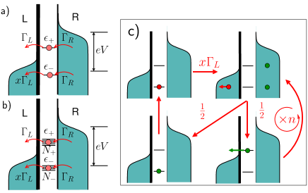
Figure 1: a) Two-terminal quantum dot with two levels. The tunneling rate from the lower level to the left lead is thermally activated due to finite occupation of the left lead. All other tunneling processes have much larger rates. Coulomb charging allows only one of the levels to be occupied. b) The same with $N_{+}$ upper levels and $N_{-}$ lower levels. c) Transport cycles leading to super-Poissonian shot noise. With a small tunneling rate $x\Gamma_{L}$ a cycle is initiated by an electron tunneling from the dot to the left lead, followed by $n$ cycles ($n=0,1,2,\ldots$) of tunneling through the upper level with probability $1/2$. Finally the process is stopped by a tunneling event from the right terminal to the lower level with probability $1/2$. In total $n+1$ charges are transfered in a cycle with a rate $x\Gamma_{L}(1/2)^{n+1}$, which explains the super-Poissonian noise and all other transport characteristics.

In this limit the system is described by a Master equation of the form

$$\frac{d}{dt}\left(\begin{array}[c]{c}P_{-}\\ P_{+}\\ P_{0}\end{array}\right)=\left(\begin{array}[c]{ccc}-x\Gamma_{L}&0&\Gamma_{R}\\ 0&-\Gamma_{L}&\Gamma_{R}\\ x\Gamma_{L}&\Gamma_{L}&-2\Gamma_{R}\end{array}\right)\left(\begin{array}[c]{c}P_{-}\\ P_{+}\\ P_{0}\end{array}\right)\equiv\hat{M}\vec{P}.$$ (2)

Here $P_{\pm}$ describes the occupation of the upper/lower level and $P_{0}$ is the probability that the island is empty. The rates are parameterized by the bare tunneling rates $\Gamma_{L/R}$ to tunnel out of the dot to the left or to tunnel onto the dot from the right. The (small) parameter $x$ is determined by the thermal occupations in the left lead: tunneling from the lower state is suppressed by a factor $x=1-f(\epsilon_{-})$, since the states in the left lead are mostly occupied.

Now we determine the counting statistics using the method of Bagrets and Nazarov bagrets:03 . We add the corresponding counting factors $\exp(i\chi)$ to the entries of the Master equation, which involve changes of the dot occupation and refer to tunneling into one of the terminals. This procedure leads to the rate matrix

$$\hat{M}(\chi)=\left(\begin{array}[c]{ccc}-x\Gamma_{L}&0&\Gamma_{R}\\ 0&-\Gamma_{L}&\Gamma_{R}\\ x\Gamma_{L}e^{i\chi}&\Gamma_{L}e^{i\chi}&-2\Gamma_{R}\end{array}\right)\,,$$ (3)

where we have chosen to count the charges in the left terminal. The counting statistics is determined from the lowest eigenvalue $\lambda_{0}(\chi)$ of $\hat{M}(\chi)$ according to

$$S(\chi)=-\lambda_{0}(\chi)t_{0}\,.$$ (4)

The eigenvalue equation reads

$$0 = (x\Gamma_{L}+\lambda)\left[\Gamma_{L}\Gamma_{R}e^{i\chi}-(\Gamma_{L}+\lambda)(2\Gamma_{R}+\lambda)\right]$$ (5)

$$+x\Gamma_{L}e^{i\chi}\Gamma_{R}(\Gamma_{L}+\lambda)\,.$$

For the present purpose, it is sufficient to determine the lowest eigenvalue perturbatively in $x\ll 1$ and to assume $\Gamma_{L}\ll\Gamma_{R}$. The counting statistics is obtained as

$$S(\chi)=-2x\Gamma_{L}t_{0}\frac{e^{i\chi}-1}{2-e^{i\chi}}\,.$$ (6)

This cumulant generating function reproduces, of course, correctly the first cumulant $C_{1}=2x\Gamma_{L}t_{0}$ and the noise $C_{2}=3C_{1}$, corresponding to a Fano factor $F=C_{2}/|C_{1}|$ of $3$.cottet:prb The first interesting observation is that the current is twice the estimate of the simple thermal tunneling rate $x\Gamma_{L}$. Furthermore, the noise corresponds to an effective charge $q_{\mathrm{eff}}=C_{2}/C_{1}=3$, which could be interpreted as a Poissonian process of 3 charges. However, we obtain the for the higher cumulants

$$C_{3}=13C_{1} C_{4}=75C_{1},$$ , (7)

$$C_{5}=541C_{1} C_{6}=4683C_{1}\,.$$ , (8)

Notably, third (and higher) cumulants obey the relation $C_{n}>q_{\mathrm{eff}}^{n-1}C_{1}$ and, consequently, the transport statistics can not be explained by a simple Poissonian process in which multiple charges of size $q_{\mathrm{eff}}$ are transfered. Note that this would follow from a counting statistics $-(x\Gamma_{L}/q_{\mathrm{eff}})(\exp(iq_{\mathrm{eff}}\chi)-1)$.

A simple physical picture emerges, if we expand the cumulant generating function (6) in terms of Poissonian processes. As a result we find

$$S(\chi)=-x\Gamma_{L}\sum_{n=1}^{\infty}\frac{1}{2^{n}}\left(e^{in\chi}-1\right)\,.$$ (9)

The counting statistics is therefore a sum of independent Poisson processes, in each of which a charge of $ne$ is transfered as signaled by the factor $\exp(in\chi)-1$. Each process is weighted with a probability $(1/2)^{n}$. This result for the statistics suggests the following interpretation (see also Fig. 1). The lower level is occupied most of the time, since it is well below the chemical potentials of the two leads. Due to Coulomb blockade the other level cannot be occupied at the same time (we assume here that the charging energy is larger than the bias voltage). At a finite temperature, there will be a small rate $\sim x\Gamma_{L}$ for the electron to hop out to the left lead. Next, the dot will be filled again with an electron from the right lead. However, as we are in the situation $eV_{R}>\epsilon_{+}$ both levels will be occupied in the next step with the same probabilities of $1/2$. In case the lower state is occupied we are back to the initial state and one charge has been transfered in this cycle, which is exactly what is happening in a single level quantum dot in the thermally activated transport regime. However, if the electron has tunneled onto the upper level, it can quickly tunnel out to the left lead and the dot is empty again and another electron can tunnel from the right terminal. Each intermediate cycle occurs with a probability $1/2$ (since two states are available) and transfers an additional charge. Therefore each full cycle has a probability $(1/2)^{n}$ and transfers $ne$ charge.

We now turn to the more general situation of a multi-level quantum dot. The level structure we assume here is depicted in Fig. 1b). As before the Coulomb energy is assumed to be so large that only one of the levels can be occupied at the same time. The levels are bunched into two groups, the lower group with $N_{-}$ levels and the upper group with $N_{+}$ levels. We will furthermore assume that the tunneling rate into and from all levels inside a group are the same. Physically this means that the maximal level spacing inside the lower group is smaller than the temperature, so that the thermal blocking factor $x=1-f(\epsilon_{-})$ is the same for all levels. For the upper group the requirement on the level spacing is less restrictive. We only have to assume that the band width of the upper group is smaller than the bias voltage.

In principle we have to account now for $N_{+}+N_{1}+1$ probabilities in the Master equations, but due to the simplifications made above, we can replace blocks containing ’upper’(’lower’) probabilities by a single equation with the rate multiplied with a factor $N_{+(-)}$, respectively. This procedure leads to the $\chi$-dependent rate matrix

$$\hat{M}(\chi)=\left(\begin{array}[c]{ccc}-x\Gamma_{L}N_{-}&0&\Gamma_{R}N_{+}\\ 0&-\Gamma_{L}N_{+}&\Gamma_{R}N_{+}\\ x\Gamma_{L}N_{-}e^{i\chi}&\Gamma_{L}N_{+}e^{i\chi}&-2\Gamma_{R}N_{+}\end{array}\right)\,,$$ (10)

As before, it is sufficient to evaluate the CGF to lowest order in $x$. Let us introduce $p=N_{+}/(N_{-}+N_{+})$, which is the relative probability that an electron tunneling from the right electrode occupies the upper level. The counting statistics (in first order in $x$) is

$$S(\chi)=\lambda_{0}(\chi)t_{0}=-x\Gamma_{L}t_{0}\frac{e^{i\chi}-1}{1-pe^{i\chi}}\,.$$ (11)

This CGF gives the first cumulant $C_{1}=x\Gamma_{L}t_{0}/(1-p)$ and the higher cumulants are

$$C_{2} = \frac{1+p}{1-p}C_{1},$$

$$C_{3} = \frac{1+4p+p^{2}}{(1-p)^{2}}C_{1},$$

$$C_{4} = \frac{(1+p)(1+10p+p^{2})}{(1-p)^{3}}C_{1},$$

$$C_{5} = \frac{1+26p+66p^{2}+26p^{3}+p^{4}}{(1-p)^{4}}C_{1},$$

$$C_{6} = \frac{(1+p)(1+56p+246p^{2}+56p^{3}+p^{4})}{(1-p)^{5}}C_{1}\,.$$

We note that the average is larger by the factor $1/(1-p)$ than the Poissonian estimate. Furthermore, higher cumulants obey the relation $C_{n}>(C_{2}/C_{1})^{n-1}C_{1}$,superproof which shows the unusual characteristics of the transport. Similar to the previous case, we can decompose the FCS into multiple Poisson processes as

$$S(\chi)=-x\Gamma_{L}(1-p)\sum_{n=1}^{\infty}p^{n-1}\left(e^{in\chi}-1\right)\,.$$ (12)

The statistics is a sum of Poissonian processes of multiple charges, weighted with probabilities $P_{n}=p^{n-1}(1-p)$. This suggests the picture depicted in Fig. 1c). The possible Poissonian processes result from a tunneling event with the small initial rate $x\Gamma_{L}$. This process is followed by $n-1$ fast cycles, in which an electron tunnels through the dot with probability $p$. Finally the fast cycle stops with a probability $1-p$. As can be seen from Eq. (12) processes of all orders contribute to the transport characteristics. A simplified description in terms of a Poissonian process, in which an effective charge tunnels, can never reproduce the observed cumulants. It is worth to emphasize, that only the complete determination of all cumulants (or equivalently the full counting statistics) can unambiguously identify this transport mechanism.

At this stage, we would like to remark that the situation, discussed here, can only occur if the levels for zero bias are situated below the Fermi level (assuming symmetric capacitive coupling). In case the levels are initially above the Fermi level, the current and the noise show the usual behaviors thielmann:03 . The corresponding counting statistics can be obtained using the method of Ref. bagrets:03, and turns out to be

$$S(\chi)=\frac{\Gamma}{2}\sqrt{1+p_{L}(e^{i\chi}-1)+p_{R}(e^{-i\chi}-1)}-\frac{\Gamma}{2}\,.$$ (13)

Here $p_{L,R}$ are the respective probabilities of a tunneling event to the left(right) and $\Gamma$ refers to the total tunneling rate. In the regime of unidirectional transport $p_{L}\gg p_{R}$ and we obtain

$$C_{1}=t_{0}\frac{\Gamma}{4}p_{L}\quad\mbox{and}\quad F=1-p_{L}/2\,.$$ (14)

The Fano factor is always between $1/2$ for the symmetric case ($p_{L}=1$) and 1 for the asymmetric case ($p_{L}\ll 1$). It follows also, that higher-order cumulants are suppressed even further. This situation is remarkably similar to transport through a noninteracting resonant level in the limit of a bias voltage much smaller than the width of the resonance.

The difference between super-Poissonian and sub-Poissonian statistics discussed here has several interesting consequences. First, we note that the second cumulant in the super-Poissonian case is enhanced by a factor $1+2N_{+}/N_{-}$. If for example $N_{-}=1$, the enhancement of the noise is a direct measure of the number of excited states within the transport window. Notably, the full information requires to study also the third (and higher) cumulants, since higher cumulants are not related to the second cumulant in a simple way. These observations are important for experimental studies of transport through molecules and other quantum dots with an unknown internal level structures. As an example we consider a molecule, in which it is not known, whether transport takes place through the lowest unoccupied molecular orbital (LUMO) or the highest unoccupied molecular orbital (HOMO), because the position of the Fermi energy of the leads is not known. The current in both cases shows a step at a threshold voltage. However, the noise is able to distinguish both situations. For transport through a multitude of LUMO levels, the noise is always sub-Poissonian, see e.g. setnoise ; thielmann:03 . However, transport through the HOMO falls in the category discussed in this work. If there are excited levels in the transport window, which cannot be occupied in equilibrium due to Coulomb repulsion, we predict a super-Poissonian noise. Thus, noise measurements may be used to distinguish transport through the HOMO or the LUMO, which show the same average current-voltage characteristics.

In summary, we have pointed out the unusual noise characteristics of the transport through a quantum dot with an internal level structure. A super-Poissonian noise results from a combination of Poissonian processes with multiple charges weighted with probabilities, depending on the internal level structure. The obtained results allow to identify the level structure, which is a useful information in molecular electronic devices. We emphasize here, that only a study of the complete statistics allows a determination of the transport mechanism underlying the super-Poissonian shot noise. While we have explored a rather simplistic model of a quantum dot, further studies will reveal in more detail what information can be obtained from current fluctuation measurements in quantum dots and molecules with a complicated internal level structure.

I acknowledge useful discussion with C. Bruder and A. Cottet. This work was supported by the Swiss NSF, the NCCR Nanoscience and the RTN Spintronics.

References

- (1) Ya. M. Blanter and M. Büttiker, Phys. Rep. 336, 1 (2000).
- (2) Quantum Noise in Mesoscopic Physics, edited by Yu. V. Nazarov (Kluwer, Dordrecht, 2003).
- (3) L. S. Levitov and G. B. Lesovik, Pis’ma Zh. Eksp. Teor. Fiz. 58, 225 (1993); L. S. Levitov, H. W. Lee, and G. B. Lesovik, J. Math. Phys. 37, 4845 (1996).
- (4) V. A. Khlus, Sov. Phys. JETP 66, 1243 (1987);G. B. Lesovik, JETP Lett. 49, 592 (1989);M. Büttiker, Phys. Rev. Lett. 65, 2901 (1990).
- (5) M. J. M. de Jong and C. W. J. Beenakker, Phys. Rev. B 49, 16070 (1994); T. Martin, Phys. Lett. A 220, 137 (1996); M. P. Anantram and S. Datta, Phys. Rev. B 53, 16390 (1996); J. Torres and T. Martin, Eur. Phys. J. B 12, 319 (1999); Fauchere ; J. Torres, T. Martin, and G. B. Lesovik, Phys. Rev. B 63, 134517 (2001); M. Schechter, Y. Imry, and Y. Levinson, Phys. Rev. B 64, 224513 (2001); X. Jehl et al., Phys. Rev. Lett. 83, 1660 (1999); X. Jehl et al., Nature 405, 50 (2000); A. A. Kozhevnikov, R. J. Schoelkopf, and D. E. Prober, Phys. Rev. Lett 84, 3398 (2000); K. E. Nagaev and M. Büttiker, Phys. Rev. B 63, 081301(R) (2001). M. P. V. Stenberg and T T. Heikkilä, Phys. Rev. B 66, 144504 (2002); F. Pistolesi, G. Bignon, and F. W. J. Hekking, cond-mat/0303165 (unpublished); F. Lefloch, C. Hoffmann, M. Sanquer, and D. Quirion, Phys. Rev. Lett. 90, 067002 (2003).
- (6) B. A. Muzykantskii and D. E. Khmelnitzkii, Phys. Rev. B 50, 3982 (1994); W. Belzig and Yu. V. Nazarov, Phys. Rev. Lett. 87, 197006 (2001); Phys. Rev. Lett. 87, 067006 (2001); J. Börlin, W. Belzig, and C. Bruder, Phys. Rev. Lett. 88, 197001 (2002); P. Samuelsson and M. Büttiker, Phys. Rev. Lett. 89, 046601 (2002); W. Belzig and P. Samuelsson, Europhys. Lett. 64, 253 (2003).
- (7) J.C. Cuevas and W. Belzig, Phys. Rev. Lett. 91, 187001 (2003); G. Johansson, P. Samuelsson and A. Ingerman, Phys. Rev. Lett. 91, 187002 (2003); J.C. Cuevas and W. Belzig, Phys. Rev. B 70, 214512 (2004); S. Pilgram and P. Samuelsson, cond-mat/0407029 (unpublished).
- (8) A. N. Korotkov, Phys. Rev. B 49, 10381 (1994); S. Hershfield, J. H. Davies, P. Hyldgaard, C. J. Stanton, and J. W. Wilkins, ibid. 47, 1967 (1993); U. Hanke, Yu. M. Galperin, K. A. Chao, and N. Zou, ibid. 48, 17209 (1993); H. Birk, M. J. M. de Jong, and C. Schönenberger, Phys. Rev. Lett. 75, 1610 (1995).
- (9) D. A. Bagrets and Yu. V. Nazarov, Phys. Rev. B 67, 085316 (2003).
- (10) B. R. Bulka, J. Martinek, G. Michalek, and J. Barnas, Phys. Rev. B 60, 12246 (1999); B. R. Bulka, Phys. Rev. B 62, 1186 (2000).
- (11) A. Cottet and W. Belzig, Europhys. Lett. 66, 405 (2004); A. Cottet, W. Belzig, and C. Bruder, Phys. Rev. Lett. 92, 206801 (2004).
- (12) G. Michalek and B. R. Bulka, Eur. Phys. J. B 28, 121 (2002); G. Kießlich, A. Wacker, and E. Schöll, Phys. Rev. B 68, 125320 (2003); S. S. Safonov, A. K. Savchenko, D. A. Bagrets, O. N. Jouravlev, Y. V. Nazarov, E. H. Linfield, and D. A. Ritchie, Phys. Rev. Lett. 91, 136801 (2003); O. Sauret and D. Feinberg, Phys. Rev. Lett. 92, 106601 (2004).
- (13) Ya. M. Blanter and M. Büttiker, Phys. Rev. B 59, 10217 (1999).
- (14) E. V. Sukhorukov, G. Burkard, and D. Loss, Phys. Rev. B 63, 125315 (2001).
- (15) M. Büttiker, Phys. Rev. B 46, 12485 (1992); for a review, see M. Büttiker, in Ref. nazarov:03 .
- (16) Y. P. Li, A. Zaslavski, D. C. Tsui, M. Santos, and M. Shayegan, Phys. Rev. B 41, 8388 (1990); E. R. Brown, IEEE Trans. Electron Devices 39, 2686 (1992); V. V. Kuznetsov, E. E. Mendez, J. D. Bruno, and J. T. Pham, Phys. Rev. B 58, 10159 (1998); G. Iannaccone, G. Lombardi, M. Macucci, and B. Pelegrini, Phys. Rev. Lett. 80, 1054 (1998);
- (17) A. Cottet, W. Belzig, and C. Bruder, Phys. Rev. B 70, 115315 (2004).
- (18) J. Koch and F. von Oppen, cond-mat/0409667 (unpublished); J. Koch, M.E. Raikh, and F. von Oppen, cond-mat/0501065 (unpublished).
- (19) A. N. Jordan and E. V. Sukhorukov, Phys. Rev. Lett. 93, 260604 (2004).
- (20) A. Thielmann, M. H. Hettler, J. König, and G. Schön, Phys. Rev. B 68, 115105 (2003); cond-mat/0406647 (unpublished).
- (21) That this relation is obeyed for all cumulants can be seen by writing , where and yields the effective charge . Since all derivatives w.r.t. of are positive, the chain rule yields .