The Spot Model for random-packing dynamics

Abstract

The diffusion and flow of amorphous materials, such as glasses and granular materials, has resisted a simple microscopic description, analogous to defect theories for crystals. Early models were based on either gas-like inelastic collisions or crystal-like vacancy diffusion, but here we propose a cooperative mechanism for dense random-packing dynamics, based on diffusing “spots” of interstitial free volume. Simulations with the Spot Model can efficiently generate realistic flowing packings, and yet the model is simple enough for mathematical analysis. Starting from a non-local stochastic differential equation, we derive continuum equations for tracer diffusion, given the dynamics of free volume (spots). Throughout the paper, we apply the model to granular drainage in a silo, and we also briefly discuss glassy relaxation. We conclude by discussing the prospects of spot-based multiscale modeling and simulation of amorphous materials.

Dedicated to Prager Medalist, Salvatore Torquato.

1 Introduction

Professor Torquato has made pioneering contributions to the characterization of random packings and their relation to properties of heterogeneous materials (Torquato, 2003). His recent work rejects the classical notion of “random close packing” of hard spheres and replaces it with the more precise concept of a “maximally random jammed state” (Torquato et al., 2000; Torquato and Stillinger, 2001; Kansal et al., 2002; Donev et al., 2004b). In these studies and others (O’Hern et al., 2002, 2003), however, the focus is on the statistical geometry of static packings, and not on the dynamics of nearly jammed packings in flowing amorphous materials.

Dense random-packing dynamics is at the heart of condensed matter physics, and yet it remains not fully understood at the microscopic level. This is in contrast to dilute random systems (gases), where Boltzmann’s kinetic theory provides a successful statistical description, based on the hypothesis of randomizing collisions for individual particles. The same single-particle theory can also be applied to molecular liquids at typical experimental time and length scales, where kinetic energy is able to fully disrupt local packings. The difficulty arises in describing liquids at very small (atomic) length and time scales, over which the trajectories of neighboring particles are strongly correlated – the so-called cage effect  (Hansen and McDonald, 1986).

This difficulty is extended to much larger length and time scales in glassy relaxation (Angell et al., 2000) and dense granular flow (Jaeger et al., 1996), where kinetic energy is insufficient to easily tear a particle away from its cage of neighbors. As a result, one must somehow describe the cooperative motion of all particles at once. In dense ordered materials (crystals), cooperative relaxation and plastic flow are mediated by defects, such as interstitials, vacancies, and dislocations, but it is not clear how to define “defects” for homogeneous disordered materials.

The challenge in describing random-packing dynamics is related to the concept of “hyper-uniform” point distributions, recently introduced by  Torquato and Stillinger (2003). In a dilute gas, particles undergo independent random walks and thus have the “uniform” distribution of a Poisson process (Hadjiconstantinou et al., 2003), where the variance of the number of particles, $N$, scales with the volume, $V$: $\mbox{Var}(N)=\langle N\rangle=\rho V$, where $\rho$ is the mean density. In a condensed phase, the particle distribution must be “hyper-uniform”, with much smaller fluctuations, proportional to the surface area: $\mbox{Var}(N)\propto V^{(d-1)/d}$, where $d=3$ is the spatial dimension, so it is clear that particles cannot fluctuate independently. In a crystal, hyper-uniformity is a property of the ideal lattice, which is preserved during diffusion and plastic flow by the motion of isolated defects. For dense disordered materials, however, no simple flow mechanism has been identified, which preserves hyper-uniformity.

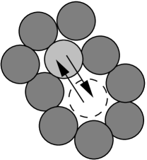
Figure 1: Eyring’s mechanism for flow in viscous liquids: A single particle jumps from one available “cage” to another by exchanging with a “void” moving in the opposite direction.

Eyring (1936) was perhaps the first to suggest a microscopic mechanism for viscous flow in liquids, analogous to vacancy diffusion in crystals. He proposed that the packing evolves when individual particles jump into available cages, thus displacing pre-existing voids, as shown in Fig. 1. Much later, the same hypothesis was put forth independently in theories of the glass transition (Cohen and Turnbull, 1959), shear flow in metallic glasses (Spaepen, 1977), granular drainage from a silo (Litwiniszyn, 1958; Mullins, 1972), and compaction in vibrated granular materials (Boutreux et al., 1998), although it is not clear that all of these authors intended for the model to be taken literally at the microscopic level. Since particles and voids simply switch places, it seems the Void Model can only be simulated on a single, fixed configuration of particles, but real flows are clearly not constrained in this way. This difficulty is apparent in the work of Caram and Hong (1991), who neglected random packings and simulated the Void Model on a lattice in an attempt to describe granular drainage.

By now, free volume theories of amorphous materials (based on voids) have fallen from favor, and experiments on glassy relaxation (Weeks et al., 2000) and granular drainage (Choi et al., 2004) have demonstrated that packing rearrangements are highly cooperative and not due to single-particle hops. In a recent theory of granular chute flows down inclined planes, Ertaş and Halsey (2002) have postulated the existence of coherent rotations, called “granular eddies” to motivate a continuum theory of the mean flow. Although the theory successfully predicts Bagnold rheology and the critical layer thickness for flow, Landry and Grest (2003) have failed to find any evidence for granular eddies in discrete-element simulations of chute flow (Landry et al., 2003).

In glass theory, Adam and Gibbs (1965) introduced the concept of regions of cooperative relaxation, whose sizes diverge at the glass transition. Modern statistical mechanical approaches are based on mode-coupling theory (Götze and Sjögren, 1992), which accurately predicts density correlation functions in simple liquids  (Kob, 1997), although a clear microscopic mechanism, which could be used in a particle simulation, has not really emerged. Cooperative rearrangements have also long been recognized in the literature on sheared glasses. Orowan (1952) was perhaps the first to postulate localized shear transformations in regions of enhanced atomic disorder. Argon (1979) later developed the idea of “intense shear transformations” at low temperature, which underlies the stochastic model of “localized inelastic transformations” (Bulatov and Argon, 1994). A similar notion of “shear transformation zones” (STZ) has also been invoked by  Falk and Langer (1998) in a continuum theory of shear response, which has recently been extended to account for free-volume creation and annihilation in glasses (Lemaître, 2002b) and granular materials (Lemaître, 2002a). This phenomenology seems to capture many universal features of amorphous materials, although the microscopic picture of “$+$” and “$-$” STZ states remains vague.

In this paper, we propose a simple model for the kinematics of dense random packings. In section 2, we introduce a general mechanism for structural rearrangements based on the concept of a diffusing “spot” of free volume. In section 3, we apply the Spot Model to granular drainage. In section 4, we analyze the diffusion of a tracer particle via a non-local, nonlinear stochastic differential equation, in the limit of an ideal gas of spots. In section 5, we derive equations for tracer diffusion in granular drainage, which depend on the density, drift, and diffusivity of spots (or free volume). We close by discussing possible applications to glasses in section 6 and spot-based multiscale modeling and simulation of amorphous materials in section 7.

2 The Spot Model

2.1 Motivation

Our intuition tells us that a particle in a dense random packing must move together with its nearest neighbors over short distances, followed by gradual cage breaking at longer distances. In simple liquids, this transition occurs at the molecular scale ($<$ nm) over very short times ($<$ ps) compared to typical experimental scales. In supercooled liquids and glasses, the time scale for structural relaxation effectively diverges and is replaced by slow, power-law decay (Angell et al., 2000; Kob, 1997; Hansen and McDonald, 1986), although the length scale for cooperative motion remains relatively small (Weeks et al., 2000). In granular drainage, cage breaking occurs slowly, over time scales comparable to the exit time from the silo, so that cooperative motion is important throughout the system at the macroscopic scale (Choi et al., 2004).

Another curious feature of granular drainage is the importance of geometry: all fluctuations in a dense flow seem to have a universal dependence on the distance dropped for a wide range of flow rates (Choi et al., 2004). In a sense, therefore, increasing the flow speed in this regime is like fast-forwarding a film, passing through the same sequence of configurations, only more quickly. The only existing theory to predict this property (as well as the mean flow profile in silo drainage) is the Void Model, since increasing the flow speed simply increases the injection rate of voids, but not their geometrical trajectories. However, the model incorrectly predicts cage breaking and mixing at the scale of individual particles. This “paradox of granular diffusion” is a fruitful starting point for a new model of random-packing dynamics (Bazant et al., 2005).

2.2 General formulation

Let us suppose that the cage effect gives rise to spatial correlations in particle velocities, with correlation coefficient, $C(r)$, for two particles separated by $r$. More generally, when there is broken symmetry, e.g. due to gravity in granular drainage, there is a correlation coefficient, $C^{\alpha\beta}_{p}(\mbox{\bf r}_{1},\mbox{\bf r}_{2})$, for the $\alpha$ velocity component of a particle at $\mbox{\bf r}_{1}$ and the $\beta$ velocity component of a particle at $\mbox{\bf r}_{2}$. Perhaps the simplest way to encode this information in a microscopic model is to imagine that particles move cooperatively in response to some extended entity – a spot – which causes a particle at $\mbox{\bf r}_{p}$ to move by

$$\Delta\mbox{\bf R}_{p}=-w(\mbox{\bf r}_{p},\mbox{\bf r}_{s})\,\Delta\mbox{\bf R}_{s}$$ (1)

when it moves by $\Delta\mbox{\bf R}_{s}$ near $\mbox{\bf r}_{s}$. Although the spot is not a “defect” per se, like a dislocation in an ordered packing, it is a collective excitation which allows a random packing to rearrange.

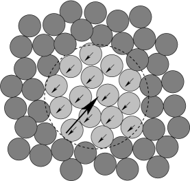
Figure 2: The spot mechanism for cooperative diffusion: A group of neighboring particles makes small correlated displacements in response to a diffusing “spot” of excess interstitial volume.

In principle, the spot influence, $w$, could be a matrix causing a smooth distribution of local translation and rotation about the spot center $\mbox{\bf r}_{s}$, but a reasonable first approximation is that it is simply a collective translation the opposite direction from the spot displacement, as illustrated in Fig. 2. In this case, $w$ is a scalar function, whose shape is roughly that of the velocity correlation function. More precisely, under some simple assumptions, we show below that $C(r)$ is the overlap integral of two spot influence functions separated by $r$. Since the spot influence is related to the cage effect, we expect that $w$ and $C$ will decay quickly with distance, for separations larger than a few particle diameters. Due to the local statistical regularity of dense random packings, we might expect a spot to retain its “shape” as it moves, in which case $w$ depend only on the separation vector, $\mbox{\bf r}_{p}^{(i)}-\mbox{\bf r}_{s}^{(j)}$, although this assumption might need to be relaxed in regions of large gradients in density or velocity.

Physically, what is a spot? Since particles move collectively in one direction, a spot must correspond to some amount of free interstitial volume (or “missing particles”) moving in the other direction. If particles are distributed with number density $\rho_{p}(\mbox{\bf r}_{p})$ and a spot at $\mbox{\bf r}_{s}$ carries a typical volume, $V_{s}(\mbox{\bf r}_{s})$, then an approximate statement of volume conservation is

$$V_{s}\Delta\mbox{\bf R}_{s}=-\int d\mbox{\bf r}_{p}\rho(\mbox{\bf r}_{p})w(\mbox{\bf r}_{p},\mbox{\bf r}_{s})\Delta\mbox{\bf R}_{p}(\mbox{\bf r}_{p}).$$ (2)

For particles distributed uniformly at volume fraction, $\phi$, this reduces to a simple expression for the local volume carried by a spot,

$$V_{s}(\mbox{\bf r}_{s})=\phi\int d\mbox{\bf r}_{p}w(\mbox{\bf r}_{p},\mbox{\bf r}_{s}),$$ (3)

which can thus be interpreted as a measure of the spot’s “total influence”.

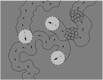
Figure 3: The trails of spots correspond to transient, reptating chains of particles.

A very simple, spot-based Monte Carlo simulation proceeds as follows. Given a distribution of (passive) particles and (active) spots, the random displacement, $\Delta\mbox{\bf R}_{s}^{(j)}$, of the $j$th spot centered at $\mbox{\bf r}_{s}^{(j)}$ induces a random displacement, $\Delta\mbox{\bf R}_{p}^{(i)}$, of the $i$th particle centered at $\mbox{\bf r}_{p}^{(i)}$:

$$\Delta\mbox{\bf R}_{p}^{(i)}=-w(\mbox{\bf r}_{p}^{(i)},\mbox{\bf r}_{s}^{(j)}+\Delta\mbox{\bf R}_{s}^{(j)})\,\Delta\mbox{\bf R}_{s}^{(j)}$$ (4)

Each spot undergoes an independent random walk, with an appropriate drift and diffusivity for free volume, which leaves in its trail a thick chain of particles reptating in the opposite direction, as shown in Fig. 3. In Eq. (4), we choose to center the spot influence on the end of its small displacement, but it is also reasonable to use the midpoint of the displacement(Rycroft et al., 2005). In the infinitesimal limit (see below), these choices are analogous to different definitions of stochastic differentials (Risken, 1996).

In principle, the drift velocity, diffusivity, and influence function of spots could depend on local variables, such as stress, and temperature (or rather, some suitable microscopic quantities related to contact forces and velocities, respectively). Spots could also interact with each other, undergo creation and annihilation, and possess a statistical distribution of sizes (or influence functions). The simplest kinematic assumption, however, which captures the basic physics of the cage effect, is that spots are identical and maintain their properties while undergoing independent (non-interacting) random walks. In particular, the constant influence function, $w(|\mbox{\bf r}_{p}-\mbox{\bf r}_{s}|)$, is chosen to be translationally invariant in space and time. It turns out that this model allows rather realistic multiscale simulations, while remaining analytically tractable.

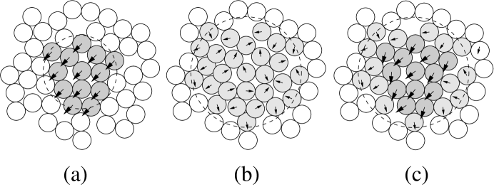
Figure 4: Multiscale simulation of densely packed (nearly) hard spheres with the Spot Model: (a) A block of neighboring particles translates opposite to the displacement of a spot of free volume; (b) the block and a shell of neighbors are allowed to relax under soft-core repulsive forces; (c) the net cooperative rearrangement combines these two steps. (Particle displacements are greatly exaggerated for clarity.)

2.3 Multiscale simulation

The simple spot mechanism above gives a reasonable description of tracer diffusion and slow cage breaking in random packings, but it does not strictly enforce packing constraints (or, more generally, inter-particle forces). As such, particles perform independent random walks in the long-time limit, which eventually leads to uniform density fluctuations with Poisson statistics. For a complete microscopic model, we must somehow preserve hyper-uniform packings.

This may be accomplished by adding a relaxation step to the spot-induced displacements, as shown in Fig. 4. First in (a), a spot displacement causes a simple correlated displacement, as described above, e.g. using Eq. (4) with some short-ranged choice of $w(r)$ with a finite cutoff. Next in (b), the affected particles and a shell of their nearest neighbors are allowed to relax under appropriate inter-particle forces, with more distant particles held fixed. For simulations of (nearly) hard grains, the most important forces come from a soft-core repulsion, which pushes particles apart only if particle begin to overlap.

Although it is not obvious a priori, the net spot-induced cooperative displacements, shown in Fig. 4(c), easily produce very realistic flowing packings, while preserving the physical picture of the model (Rycroft et al., 2005). In practice, the correlated nature and small size of the spot-induced block displacements results in very small and infrequent particle overlaps, only near the edges of the spot, where some shear occurs with the background packing. As a result, it seems the details of the relaxation are not very important, although this issue merits further investigation. In any case, the algorithm is interesting in its own right as a method of multiscale modeling, since it combines a macroscopic simulation of simple extended objects (spots) with localized, microscopic simulations of particles.

3 Application to Granular Drainage

3.1 Spot parameters

The classical Kinematic Model for the mean velocity in granular drainage (Nedderman, 1991), which compares fairly well with experiments (Tüzün and Nedderman, 1979; Samadani et al., 1999; Choi et al., 2005), postulates that the mean downward velocity, $v$, satisfies a linear diffusion equation,

$$\frac{\partial v}{\partial z}=b\,\mbox{\boldmath{$\nabla$}}_{\perp}^{2}v$$ (5)

where the vertical distance $z$ plays the role of “time” and the horizontal dimensions (with gradient, $\mbox{\boldmath{$\nabla$}}_{\perp}$) play the role of “space”. The microscopic justification for Eq. (5) is the Void Model of Litwiniszyn (1958, 1963) and Mullins (1972, 1974), where particle-sized voids perform directed random walks upward from the orifice. As discussed above, this microscopic mechanism is firmly contradicted by particle-tracking experiments (Choi et al., 2004), but, as shown below, a similar macroscopic flow equation can be derived from the Spot Model, where spot diffuse upward with a (horizontal) diffusion length,

$$b=\frac{\mbox{Var}(\Delta\mbox{\bf x}_{s})}{2d_{h}\Delta z_{s}}$$ (6)

where $\Delta\mbox{\bf x}_{s}$ is the random horizontal displacement of a spot as it rises by $\Delta z_{s}$ and $d_{h}=2$ is the horizontal dimension. A typical value for 3 mm glass beads is $b\approx 1.3d$, where $d$ is the particle diameter.

The shape of the spot influence function can be inferred from measurements of spatial velocity correlations in experiments (Bazant et al., 2005) or simulations by the discrete-element method (DEM) (Rycroft et al., 2005). The simplest assumption is a uniform spherical influence with a finite cutoff,

$$w(r)=\left\{\begin{array}[]{ll}w&r<d_{s}/2\\ 0&r>d_{s}/2\end{array}\right.$$ (7)

where experiments and simulations find $d_{s}\approx 5d$. This is consistent with our interpretation of the spot mechanism in terms of the cage effect, where a particle moves with its nearest neighbors. The typical number of particles affected by a spot,

$$N=\phi\left(\frac{d_{s}}{d}\right)^{3},$$ (8)

is thus $N\approx 72$, for $\phi\approx 0.58$.

For a uniform spot, the condition of volume conservation, Eq. (2), reads

$$V_{s}\,(\Delta\mbox{\bf x}_{s},\Delta z_{p})=-N\,V_{p}\,(\Delta\mbox{\bf x}_{p},\Delta z_{p}).$$ (9)

Using Eq. (1), this provides an expression for the spot influence,

$$w=\frac{V_{s}}{NV_{p}}\approx\frac{\Delta\phi}{\phi^{2}}$$ (10)

in terms of $\Delta\phi$, the change in local volume fraction due to the presence of a single spot. In discrete-element simulations of granular spheres in silo drainage (Rycroft et al., 2005), the local volume fraction varies in the range, $\phi=0.565-0.605$, within the rough bounds of jamming, $\phi=0.63$  (Torquato et al., 2000; Kansal et al., 2002; O’Hern et al., 2002, 2003), and random loose packing, $\phi=0.55$  (Onoda and Liniger, 1990). If we attribute $\Delta\phi/\phi=1\%$ to a single spot, then we find $w\approx 0.017$, but, if many spots, say $N_{s}=10$, can overlap, then this estimate is reduced by $1/N_{s}$. We thus expect, $w=10^{-3}-10^{-2}$, which can be tested against experiments.

We can also use Eqs. (9)-(10) to infer $w$ from a measurement of the horizontal particle diffusion length:

$$b_{p}=\frac{\mbox{Var}(\Delta\mbox{\bf x}_{p})}{2d_{h}|\Delta z_{p}|}=\frac{w^{2}\mbox{Var}(\Delta\mbox{\bf x}_{s})}{2d_{h}w\Delta z_{s}}=w\,b$$ (11)

Discrete-element simulations (Rycroft et al., 2005) and particle-tracking experiments (Choi et al., 2004) for similar flows yield $w=b_{p}/b=0.00286d/1.14d=0.00250$ and $w=d/b\mbox{Pe\hskip 1.0pt}_{x}=d/(1.3d)(321)=0.0024$, respectively (where $\mbox{Pe\hskip 1.0pt}_{x}$ is a Péclet number). These values are consistent with the predictions of the model.

A spot’s influence is related to the free volume it carries by Eq. (3). In the case of a uniform spot of diameter, $d_{s}$, its total free volume is given by

$$V_{s}=\frac{\pi\phi wd_{s}^{3}}{6}$$ (12)

which is related to the particle volume, $V_{p}$, by

$$\frac{V_{s}}{V_{p}}=w\phi\left(\frac{d_{s}}{d}\right)^{3}=wN.$$ (13)

For dense granular drainage, the typical values $N=72$ and $w=0.0025$ imply $V_{s}=0.18V_{p}$, so a spot carries only around one fifth of a particle volume, spread out over a region of roughly five particle diameters. This delocalized picture of free volume diffusion is radically different from the classical Void Model, which is the (unphysical) limit where $V_{s}=V_{p}$ and $N=w=1$.

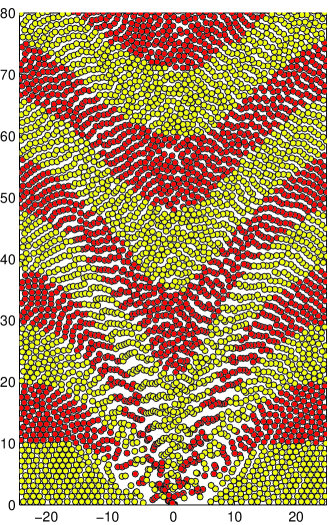
(a) (b)

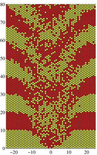
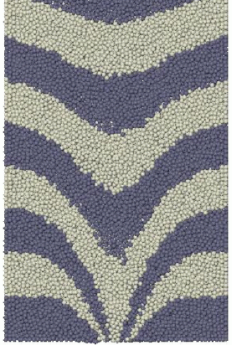
(c) (d)

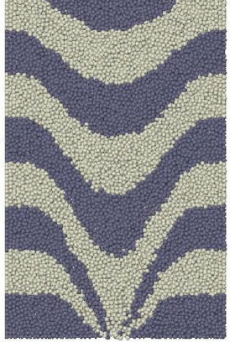
Figure 5: Simulations of granular drainage in a quasi-two-dimensional silo. Top: Two-dimensional simulations using (a) the Spot Model without packing constraints and (b) the Void Model (Bazant et al., 2005). Bottom: Three-dimensional simulations using (c) the Spot Model with multiscale relaxation and (d) the Discrete Element Method for frictional, visco-elastic spheres (Rycroft et al., 2005). Particles are colored according to their initial positions in horizontal stripes, $10d$ thick.

3.2 Spot simulations

As described above, the Spot Model can be successfully calibrated for granular drainage to enable very simple and efficient simulations. First, we consider the basic mechanism in Fig. 2 and Eq. (4) applied to granular drainage in a quasi-two-dimensional silo with a narrow opening, far from the side walls, as in the experiments of Samadani et al. (1999) and Choi et al. (2004). For simplicity, we simulate the model in two dimensions ($d_{h}=1$) using uniform spots with the parameters determined from experiments above ($w=0.0024$, $d_{s}=5d$, $b=1.3d$). The simulation begins with a random packing of identical disks, colored with horizontal stripes ($10d$ thick) to aid in visualizing the subsequent evolution.

A snapshot of the spot simulation at a later time is shown in Fig. 5(a). For comparison, a simulation of the same situation with the Void Model on a two-dimensional lattice, following Caram and Hong (1991), is shown in Fig. 5(b), along with the central slice of a three-dimensional DEM simulation ($15d$ thick) in Fig. 5(d), which is very similar to the experiment. Although the mean flow profile is similar in the spot and void simulations and reasonably close to experiment, the void simulation displays far too much diffusion and cage breaking, since the initial horizontal stripes are completely mixed down to the single particle level inside the flow region. In contrast, the interfaces between the colored layers remain fairly sharp in the spot simulation, as in experiments and the DEM simulations. Tracer diffusion is described fairly well by the spot simulation, although the lack of packing constraints eventually leads to the loss of hyper-uniformity, as particles begin to overlap and open gaps in the lower side regions of highest shear. For more details, see Bazant et al. (2005).

Next, we consider the multiscale spot algorithm in Fig. 4, with an internal relaxation step, applied to a three-dimensional drainage simulation, starting from the same initial condition and geometry as the DEM simulation in Fig. 5(d). The simplest possible relaxation scheme is to push any pair of overlapping particles in a relaxation zone (a sphere of diameter, $d_{s}+4d$) apart by a displacement, $\alpha(d-r)$ proportional to the overlap, $d-r$, while keeping particles fixed outside a sphere of diameter, $d_{s}+2d$. A spot simulation with similar parameters as above, including such a relaxation step with $\alpha=0.8$, is shown in Fig. 5(c). The rate of introducing spots at the orifice and their upward drift velocity has also been calibrated for comparison to the DEM simulation, at the same instant in time.

Clearly, the simple multiscale relaxation step is able to preserve realistic random packings, and in many ways the spot simulation in Fig. 5(c) is indistinguishable from the much more computationally demanding simulation in Fig. 5(d). Not only are the mean velocity profile and diffusion length reproduced, but so are various microscopic statistics of the packing geometry, such as the two-body and three-body correlation functions (Rycroft et al., 2005). These surprising results are quite insensitive to the details of the relaxation step, apparently due to the very small and infrequent particle overlaps which arise from the cooperative mechanism in the spot simulation. Another, deeper reason may be that the geometry of dense flowing random packings has universal features, which are achieved by the totally different dynamics of spot and DEM simulations.

4 Mathematical analysis of diffusion

4.1 A stochastic differential equation

In this section, we return to the general formulation of the Spot Model and analyze tracer diffusion in the continuum limit. It is clear from the simulations in Fig. 5 that the basic model in Fig. 2 gives a reasonable description of the dynamics of a single particle tracer, even though the multiscale relaxation step in Fig. 4 is needed to preserve realistic packings. The relatively small size of the relaxation displacements makes it reasonable to regard them a small additional “noise” in a mathematical analysis of tracer diffusion. Here, we will neglect this small (but complicated) noise and view its average effect as incorporated statistically into the spot influence function, $w(\mbox{\bf r}_{p},\mbox{\bf r}_{s})$, in Eq. (4).

We begin by partitioning space as shown Fig. 6, where the $n$th volume element, $\Delta V_{s}^{(n)}$, centered at $\mbox{\bf r}_{s}^{(n)}$ contains a random number, $\Delta N_{s}^{(n)}$, of spots at time $t$ (typically one or zero). In a time interval, $\Delta t$, suppose that the $j$th spot in the $n$th volume element makes a random displacement, $\Delta\mbox{\bf R}_{s}^{(j,n)}$ (which could be zero). According to Eq. (4), the total displacement, $\Delta\mbox{\bf R}_{p}$, of a particle at $\mbox{\bf r}_{p}$ in time $\Delta t$ is then given by a sum of all the random displacements induced by nearby moving spots,

$$\Delta\mbox{\bf R}_{p}=-\sum_{n}\sum_{j=1}^{\Delta N_{s}^{(n)}}w(\mbox{\bf r}_{p},\mbox{\bf r}_{s}^{(n)}+\Delta\mbox{\bf R}_{s}^{(j,n)})\Delta\mbox{\bf R}_{s}^{(j,n)}.$$

(14)

Note that the spatio-temporal distribution of spots, $\Delta N_{s}^{(n)}$, is another source of randomness, in addition to the individual spot displacements, $\Delta\mbox{\bf R}_{s}^{(j,n)}$, so that each particle displacement is given by a random sum of random variables.

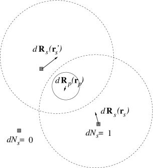
Figure 6: Sketch of a particle interacting with a collection of passing spots, showing some of the quantities involved in the nonlocal SDE, Eq.   (4.1).

In the limit of infinitesimal displacements, we arrive at a non-local, nonlinear stochastic differential equation (SDE):

$$d\mbox{\bf R}_{p}(t) = -\int dN_{s}(\mbox{\bf r}_{s},t)$$

$$w(\mbox{\bf r}_{p}(t),\mbox{\bf r}_{s}+d\mbox{\bf R}_{s}(\mbox{\bf r}_{s},t))\,d\mbox{\bf R}_{s}(\mbox{\bf r}_{s},t),$$

where the stochastic integral is defined by the usual limit (infinitely refined partition of space) of the random Riemann sum in Eq. (14). This equation differs from standard nonlinear SDEs (Risken, 1996) in two basic ways: (i) The tracer trajectory,

$$\mbox{\bf r}_{p}(t)=\int_{\tau=0}^{t}d\mbox{\bf R}_{p}(\tau)$$ (16)

is passively driven by a stochastic distribution of moving influences (spots), $dN_{s}(\mbox{\bf r}_{s},t)$, which evolves in time and space, rather than by some internal source of independent noise, and (ii) the stochastic differential, $d\mbox{\bf R}_{p}(t)$, is given by a non-local integral over other stochastic differentials, $d\mbox{\bf R}_{s}(\mbox{\bf r}_{s},t)$, associated with these moving influences, which lie at positions, $\mbox{\bf r}_{s}$, at finite distances away from the particle at $\mbox{\bf r}_{p}$.

4.2 A Fokker-Planck equation

In general, the various stochastic differentials in Equation (4.1) are correlated, which significantly complicates analysis. Here, we will make the reasonable first approximation of an ideal gas of spots, where the tracer particle sees an independent, random configuration of non-interacting spots at each infinitesimal time step. As in an ideal gas (Hadjiconstantinou et al., 2003), spots are thus distributed according to a Poisson process with a given mean density, $\rho_{s}(\mbox{\bf r}_{s},t)$. In addition to neglecting correlations caused by interactions between spots, we disregard the following facts: (i) The distribution of spots in space, $\{dN_{s}(\mbox{\bf r}_{s},t)\}$, at time $t$ depends explicitly on the distribution and displacements at the previous time, $t-dt$, via the spot random walks; (ii) Each spot, due to its finite range of influence, affects the same particle for a finite period of time, so any persistence (autocorrelation) in the spot trajectory is transferred to the particles, in a nonlinear fashion controlled by $w(\mbox{\bf r}_{p},\mbox{\bf r}_{s})$.

In the spot-gas approximation, the tracer particle performs a random walk with independent (but non-identically distributed) displacements, which depend non-locally on a Poisson process for finding spots. Therefore, the propagator, $P_{p}(\mbox{\bf r},t|\mbox{\bf r}_{0},t_{0})$, which gives the probability density of finding the particle at r at time $t$ after being at $\mbox{\bf r}_{0}$ at time $t_{0}$, satisfies the following Fokker-Planck equation (Risken, 1996),

$$\frac{\partial P_{p}}{\partial t}+\mbox{\boldmath{$\nabla$}}\cdot(\mbox{\bf u}_{p}P_{p})=\mbox{\boldmath{$\nabla$}}\mbox{\boldmath{$\nabla$}}:(\mbox{\bf D}_{p}P_{p}),$$ (17)

with drift velocity,

$$\mbox{\bf u}_{p}(\mbox{\bf r},t)=\frac{\langle d\mbox{\bf R}_{p}(\mbox{\bf r},t)\rangle}{dt}=\lim_{\Delta t\rightarrow 0}\frac{\langle\Delta\mbox{\bf R}_{p}(\mbox{\bf r},t)\rangle}{\Delta t},$$ (18)

and diffusivity tensor,

$$\mbox{\bf D}_{p}^{\alpha\beta}(\mbox{\bf r},t)=\frac{\langle dR_{p}^{\alpha}dR_{p}^{\beta}\rangle}{2\,dt}.$$ (19)

(Here $\mbox{\boldmath{$\nabla$}}\mbox{\boldmath{$\nabla$}}:\mbox{\bf A}$ denotes $\sum_{\alpha}\sum_{\beta}\frac{\partial^{2}A^{\alpha\beta}}{\partial{x_{\alpha}}\partial{x_{\beta}}}$.) The Fokker-Planck coefficients may be calculated by taking the appropriate expectations using Eq. (14) in the limits $\Delta V_{s}^{(n)}\rightarrow 0$ and $\Delta t\rightarrow 0$ (in that order), which is straightforward since we assume that spots do not interact. Here, the spot displacements, $\Delta\mbox{\bf R}_{s}^{(j)}(\mbox{\bf r}_{s}^{(n)})$, and the local numbers of spots, $\Delta N_{s}^{(n)}$, are independent random variables in each time interval, and they are independent of the same variables at earlier times.

In order to calculate the drift velocity, we need only the mean spot density, $\rho_{s}(\mbox{\bf r}_{s},t)$, defined by $\langle\Delta N_{s}^{(n)}\rangle=\rho_{s}(\mbox{\bf r}_{s},t)\,\Delta V_{s}^{(n)}$. The result,

$$\mbox{\bf u}_{p}(\mbox{\bf r}_{p},t) = -\int dV_{s}\,w(\mbox{\bf r}_{p},\mbox{\bf r}_{s})\,\left[\rho_{s}(\mbox{\bf r}_{s},t)\mbox{\bf u}_{s}(\mbox{\bf r}_{s},t)\right.$$ (20)

$$\left.-2\,\mbox{\bf D}_{s}(\mbox{\bf r}_{s},t)\cdot\mbox{\boldmath{$\nabla$}}\rho_{s}(\mbox{\bf r}_{s},t)\right]$$

exhibits two sources of drift. The first term in the integrand is a particle drift velocity, which opposes the spot drift velocity,

$$\mbox{\bf u}_{s}(\mbox{\bf r},t)=\frac{\langle d\mbox{\bf R}_{s}(\mbox{\bf r},t)\rangle}{dt}.$$ (21)

as in Eq. (9). The second term, which depends on the spot diffusion tensor,

$$\mbox{\bf D}_{s}^{(i,j)}(\mbox{\bf r},t)=\frac{\langle dR_{s}^{(i)}dR_{s}^{(j)}\rangle}{2\,dt},$$ (22)

is a “noise-induced drift”, typical of nonlinear SDEs (Risken, 1996), which causes particles to climb gradients in the spot density. This extra drift is crucial to ensure that particles eventually move toward the source of spots, e.g. the orifice in granular drainage. Both contributions to the drift velocity in Eq. (20) are averaged non-locally over a finite region, weighted by the spot influence function, $w(\mbox{\bf r}_{p},\mbox{\bf r}_{s})$.

In order to calculate the diffusivity tensor, we also need information about fluctuations in the spot density. From the spot-gas approximation, we have

$$\langle\Delta N_{s}^{(n)}\Delta N_{s}^{(m)}\rangle=\delta_{m,n}\langle(\Delta N_{s}^{(n)})^{2}\rangle=O((\Delta V_{s}^{(n)})^{\nu}),$$

where $\nu=1$ for a Poisson process and $\nu<1$ for a hyper-uniform process (Torquato and Stillinger, 2003). It turns out that such fluctuations do not contribute to the diffusion tensor (in more than one dimension), and the result is

$$\mbox{\bf D}_{p}(\mbox{\bf r}_{p},t)=\int dV_{s}w(\mbox{\bf r}_{p},\mbox{\bf r}_{s})^{2}\rho_{s}(\mbox{\bf r}_{s},t)\mbox{\bf D}_{s}(\mbox{\bf r}_{s},t).$$

(23)

Note that the influence function, $w$, appears squared in Eq. (23) and linearly in Eq. (20), which causes the Péclet number for tracer particles to be of order $w$ smaller than that of spots (or free volume), as in Eq. (11).

Higher-order terms a Kramers-Moyall expansion generalizing Eq. (17) for finite independent displacements, which do depend on fluctuations in the spot density, are straightforward to calculate, but beyond the scope of this paper. Such terms are usually ignored because, in spite of improving the approximation, they tend to produce small negative probabilities in the tails of distributions (Risken, 1996). In granular materials, however, velocity gradients can be highly localized, so the correction terms could be useful.

4.3 Spatial velocity correlation tensor

For any stochastic process representing the motion of a single particle, it is well-known that transport coefficients can be expressed in terms of temporal correlation functions via the Green-Kubo relations (Risken, 1996). For example, the diffusivity tensor in a uniform flow is given by the time integral of the velocity auto-correlation tensor,

$$D_{p}^{\alpha\beta}=\int_{0}^{\infty}dt\langle U_{p}^{\alpha}(t)U_{p}^{\beta}(0)\rangle$$ (24)

where $\mbox{\bf U}_{p}(t)=\{U_{p}^{\alpha}\}=d\mbox{\bf R}_{p}/dt$ is the stochastic velocity of a particle. (A similar relation holds for spots.)

In the Spot Model, nearby particles move cooperatively, so the transport properties of the collective system also depend on the two-point spatial velocity correlation tensor,

$$C_{p}^{\alpha\beta}(\mbox{\bf r}_{1},\mbox{\bf r}_{2})=\frac{\langle U_{p}^{\alpha}(\mbox{\bf r}_{1})U_{p}^{\beta}(\mbox{\bf r}_{2})\rangle}{\sqrt{\langle U_{p}^{\alpha}(\mbox{\bf r}_{1})^{2}\rangle\langle U_{p}^{\beta}(\mbox{\bf r}_{2})^{2}\rangle}}$$ (25)

which is normalized so that $C_{p}^{\alpha\beta}(\mbox{\bf r},\mbox{\bf r})=1$. We emphasize that the expectation above is conditional on finding two particles at $\mbox{\bf r}_{1}$ and $\mbox{\bf r}_{2}$ at a given moment in time and includes averaging over all possible spot distributions and displacements. Substituting the SDE (4.1) into Eq. (25) yields

$$C_{p}^{\alpha\beta}(\mbox{\bf r}_{1},\mbox{\bf r}_{2}) =\int dV_{s}\,\rho_{s}(\mbox{\bf r}_{s})w(\mbox{\bf r}_{1},\mbox{\bf r}_{s})w(\mbox{\bf r}_{2},\mbox{\bf r}_{s})$$ (26)

$$D_{s}^{\alpha\beta}(\mbox{\bf r}_{s})/\sqrt{D_{p}^{\alpha\beta}(\mbox{\bf r}_{1})D_{p}^{\alpha\beta}(\mbox{\bf r}_{2})}$$

assuming independent spot displacements.

Equation (26) is an integral relation for cooperative diffusion, which relates the spatial velocity correlation tensor to the spot (or free volume) diffusivity tensor via integrals of the spot influence function, $w(\mbox{\bf r}_{p},\mbox{\bf r}_{s})$. If the statistical dynamics of spots is homogeneous (in particular, if $\mbox{\bf D}_{s}$ is constant), then the relation simplifies:

$$C^{\alpha\beta}_{p}(\mbox{\bf r}_{1},\mbox{\bf r}_{2})=$$ (27)

$$\frac{\int dV_{s}\,\rho_{s}(\mbox{\bf r}_{s})\,w(\mbox{\bf r}_{1},\mbox{\bf r}_{s})\,w(\mbox{\bf r}_{2},\mbox{\bf r}_{s})}{\sqrt{\int dV_{s}\,\rho_{s}(\mbox{\bf r}_{s})\,w(\mbox{\bf r}_{1},\mbox{\bf r}_{s})^{2}\,\int dV_{s}^{\prime}\,\rho_{s}(\mbox{\bf r}_{s}^{\prime})\,w(\mbox{\bf r}_{2},\mbox{\bf r}_{s}^{\prime})^{2}}}.$$

if also the tensor is diagonal, $D_{s}^{\alpha\beta}\propto\delta_{\alpha,\beta}$. If the statistical dynamics of particles is also homogeneous, as in a uniform flow ($\rho_{s}=$ constant), then it simplifies even further:

$$C^{\alpha\beta}_{p}(\mbox{\bf r})=\frac{\int dV_{s}\,w(\mbox{\bf r}-\mbox{\bf r}_{s})\,w(-\mbox{\bf r}_{s})}{\int dV_{s}\,w(\mbox{\bf r}_{s})^{2}}$$ (28)

where we have assumed that the spot influence function, and thus the correlation tensor, is translationally invariant ($\mbox{\bf r}=\mbox{\bf r}_{1}-\mbox{\bf r}_{2}$). In this limit, as mentioned above, the velocity correlation function is simply given by the (normalized) overlap integral for spot influences separated by r.

4.4 Relative diffusion of two tracers

The spatial velocity correlation function affects many-body transport properties. For example, the relative displacement of two tracer particles, $\mbox{\bf r}=\mbox{\bf r}_{1}-\mbox{\bf r}_{2}$, has an associated diffusivity tensor given by,

$$D^{\alpha\beta}(\mbox{\bf r}_{1},\mbox{\bf r}_{2}) = D_{p}^{\alpha\beta}(\mbox{\bf r}_{1})+D_{p}^{\alpha\beta}(\mbox{\bf r}_{2})$$

$$-2\,C^{\alpha\beta}_{p}(\mbox{\bf r}_{1},\mbox{\bf r}_{2})\,\sqrt{D_{p}^{\alpha\alpha}(\mbox{\bf r}_{1})D_{p}^{\beta\beta}(\mbox{\bf r}_{2})}$$

In a uniform flow, the diagonal components take the simple form

$$D^{\alpha\alpha}(\mbox{\bf r})=2\,D^{\alpha\alpha}_{p}\left(1-C^{\alpha\alpha}_{p}(\mbox{\bf r})\right)$$ (30)

which may be used above to estimate the cage-breaking time, as the expected time for two particles diffuse apart by more than one particle diameter. A more detailed calculation of the relative propagator, $P(\mbox{\bf r},t|\mbox{\bf r}_{0},t_{0})$, neglecting temporal correlations (as above) would start from the associated Fokker-Planck equation,

$$\frac{\partial P(\mbox{\bf r},t)}{\partial t}=\mbox{\boldmath{$\nabla$}}\mbox{\boldmath{$\nabla$}}:\left(\mbox{\bf D}(\mbox{\bf r})P(\mbox{\bf r},t)\right)$$ (31)

with a delta-function initial condition. (In a non-uniform flow, one must also account for noise-induced drift and motion of the the center of mass.) This analysis does not enforce packing constraints, so it allows for two particles to be separated by less than one diameter. A hard-sphere repulsion may be approximated by a reflecting boundary condition at $|\mbox{\bf r}|=d$ when solving equations such as (31), but there does not seem to be any simple way to enforce inter-particle forces exactly in the analysis.

5 Tracer diffusion in granular drainage

5.1 Statistical dynamics of spots

The analysis in the previous section makes no assumptions about spots, other than the existence of well-defined local mean density, mean velocity, and diffusion tensor, which may depend on time and space. As such, the results may have relevance for a variety of dense disordered systems exhibiting cooperative diffusion (see below). In this section, we apply the model to the specific case of granular drainage, in which spots diffuse upward from a silo orifice, as in Fig. 5. Our goal here is simply to show how to derive continuum equations from the Spot Model in a particular case, but not to study any solutions in detail.

For simplicity, let us assume that each spot undergoes mathematical Brownian motion with a vertical drift velocity, $\mbox{\bf u}_{s}=v_{s}\hat{z}$, and a diagonal diffusion tensor,

$$\mbox{\bf D}_{s}=\left(\begin{array}[]{ccc}D_{s}^{\perp}&0&0\\ 0&D_{s}^{\perp}&0\\ 0&0&D_{s}^{\|}\end{array}\right)$$ (32)

which allows for a different diffusivity in the horizontal ($\perp$) and vertical ($\|$) directions due to symmetry breaking by gravity. In that case, the propagator for a single “spot tracer”, $P_{s}(\mbox{\bf x},z,t|\mbox{\bf x}_{0},z_{0},t)$, satisfies another Fokker-Planck equation,

$$\frac{\partial P_{s}}{\partial t}+\frac{\partial}{\partial z}\left(v_{s}P_{s}\right)=\mbox{\boldmath{$\nabla$}}^{2}_{\perp}\left(D_{s}^{\perp}P_{s}\right)+\frac{\partial^{2}}{\partial z^{2}}\left(D_{s}^{\|}P_{s}\right).$$

(33)

The coefficients may depend on space (e.g. larger velocity above the orifice than near the stagnant region), as suggested by the shape of some experimental density waves  (Baxter et al., 1989).

The geometrical spot propagator, ${\cal P}_{s}(\mbox{\bf x},|z,\mbox{\bf x}_{0},z_{0})$, is the conditional probability of finding a spot at horizontal position x once it has risen to a height $z$ from an initial position $(\mbox{\bf x}_{0},z_{0})$. For constant $v_{s}$ and $\mbox{\bf D}_{s}$, the geometrical propagator satisfies the diffusion equation,

$$\frac{\partial{\cal P}_{s}}{\partial z}=b\,\mbox{\boldmath{$\nabla$}}^{2}_{\perp}{\cal P}_{s}$$ (34)

where $b=D_{s}^{\perp}v_{s}$ is the kinematic parameter. If spots move independently, this equation is also satisfied by the steady-state mean spot density, $\rho_{s}(\mbox{\bf x},z)$, analogous to Eq. (5) of the Kinematic Model. However, the mean particle velocity in the Spot Model, Eq. (20), is somewhat different, as it involves nonlocal effects (see below).

The time-dependent mean density of spots, $\rho_{s}(\mbox{\bf x},z,t)$, depends on the mean spot injection rate, $Q(\mbox{\bf x}_{0},z_{0},t)$ (number/area$\times$time), which may vary in time and space due to complicated effects such as arching and jamming near the orifice. It is natural to assume that spots are injected at random points along the orifice (where they fit) according to a space-time Poisson process with mean rate, $Q$. In that case, if spots do not interact, the spatial distribution of spots within the silo at time $t$ is also a Poisson process with mean density,

$$\rho_{s}(\mbox{\bf x},z,t) = \int d\mbox{\bf x}_{0}\int dz_{0}\int_{t_{0}<t}dt_{0}$$

$$Q(\mbox{\bf x}_{0},z_{0},t)\,P_{s}(\mbox{\bf x},z,t|\mbox{\bf x}_{0},z_{0},t_{0}).$$

For a point-source of spots (i.e. an orifice roughly one spot wide) at the origin with flow rate, $Q_{0}(t)$ (number/time), this reduces to

$$\rho_{s}(\mbox{\bf x},z,t)=\int_{t_{0}<t}dt_{0}\,Q_{0}(t_{0})\,P_{s}(\mbox{\bf x},z,t|0,0,t_{0}),$$

(36)

where $P_{s}$ is the usual Gaussian propagator for Eq. (33) in the case of constant $u_{s}$ and $\mbox{\bf D}_{s}$. In reality, spots should weakly interact, but the success of the Kinematic Model suggests that spots diffuse independently as a first approximation in granular drainage (Choi et al., 2005).

5.2 Statistical dynamics of particles

Integral formulae for the drift velocity and diffusivity tensor of a tracer particle may be obtained by substituting the spot density which solves Eq. (5.1) into the general expressions  (20) and (23), respectively. For example, if spots only diffuse horizontally ($D_{s}^{\|}=0$), then the mean downward velocity of particles is given by

$$v_{p}(\mbox{\bf r},t)=\int dV_{s}\,w(\mbox{\bf r}_{p},\mbox{\bf r}_{s})\,\rho_{s}(\mbox{\bf r}_{s},t)\,v_{s}(\mbox{\bf r}_{s},t)$$ (37)

Note that the mean particle velocity is a nonlocal average of nearby spot drift velocities.

For simplicity, let us consider a bulk region where the spot density varies on scales much larger than the spot size. In this limit, the integrals over the spot influence function reduce to the following “interaction volumes”:

$$V_{k}(\mbox{\bf r})=\int d\mbox{\bf r}_{s}w(\mbox{\bf r},\mbox{\bf r}_{s})^{k}$$ (38)

for $k=1,2$. (Note that $V_{1}=V_{s}$ above.) The equation for tracer-particle dynamics (17) then takes the form,

$$\frac{\partial P_{p}}{\partial t} = \frac{\partial}{\partial z}\left[\left(v_{s}\rho_{s}-2D_{s}^{\|}\frac{\partial\rho_{s}}{\partial z}\right)V_{1}P_{p}\right]$$

$$-2\mbox{\boldmath{$\nabla$}}_{\perp}\cdot\left(D_{s}^{\perp}(\mbox{\boldmath{$\nabla$}}_{\perp}\rho_{s})V_{1}P_{p}\right)$$

$$\frac{\partial^{2}}{\partial z^{2}}\left(D_{s}^{\|}\rho_{s}V_{2}P_{p}\right)+\mbox{\boldmath{$\nabla$}}^{2}_{\perp}\left(D_{s}^{\perp}\rho_{s}V_{2}P_{p}\right).$$

Again, it is clear that rescaling the spot density is equivalent to rescaling time.

When the spot dynamics is homogeneous (i.e. $u_{s}$ and $\mbox{\bf D}_{s}$ are constants), Equation (5.2) simplifies further:

$$\frac{1}{v_{s}V_{s}}\frac{\partial P_{p}}{\partial t} = \left(\frac{\partial}{\partial z}+b_{p}^{\perp}\mbox{\boldmath{$\nabla$}}^{2}+b_{p}^{\|}\frac{\partial^{2}}{\partial z^{2}}\right)(\rho_{s}P_{p})\ \ \$$

$$-2b^{\perp}\mbox{\boldmath{$\nabla$}}\cdot(P_{p}\mbox{\boldmath{$\nabla$}}\rho_{s})-2b^{\|}\frac{\partial}{\partial z}\left(P_{p}\frac{\partial\rho_{s}}{\partial z}\right)$$

where $b^{\perp}=b=D_{s}^{\perp}/v_{s}$ and $b^{\|}=D_{s}^{\|}/v_{s}$ are the spot diffusion lengths and $b_{p}^{\perp}=b_{p}V_{2}/V_{1}$ and $b_{p}^{\|}=b^{\|}V_{2}/V_{1}$ are the particle diffusion lengths. In this approximation, the latter are given by the simple formula,

$$\frac{b_{p}^{\perp}}{b^{\perp}}=\frac{b_{p}^{\|}}{b^{\|}}=\frac{\int dV_{s}\,w(\mbox{\bf r},\mbox{\bf r}_{s})^{2}}{\int dV_{s}w(\mbox{\bf r},\mbox{\bf r}_{s})}$$ (41)

which generalizes Eq. (11) for a uniform spot with a sharp cutoff. The physical meaning of the diffusion lengths becomes more clear in the limit of uniform flow, $\rho_{s}=$ constant. In terms of the position in a frame moving with the mean flow, $\zeta=v_{p}t-z$, where $v_{p}=v_{s}V_{s}\rho_{s}$, we arrive at a simple diffusion equation,

$$\frac{\partial P_{p}}{\partial\zeta}=\left(b_{p}^{\perp}\mbox{\boldmath{$\nabla$}}_{\perp}^{2}+b_{p}^{\|}\frac{\partial^{2}}{\partial z^{2}}\right)P_{p},$$ (42)

where $\zeta$, the mean distance dropped, acts like time, consistent with the experimental findings of Choi et al. (2004).

6 Possible application to glasses

We have seen that the Spot Model, in its simplest form, accurately reproduces the kinematics of bulk granular drainage, so it is tempting to speculate that it might be extended to flows in other amorphous materials. In this section, we briefly consider evidence for spot-like dynamics in glasses, but we leave further extensions of the Spot Model for future work.

Experiments have revealed ample signs of “dynamical heterogeneity” in supercooled liquids and glasses (Hansen and McDonald, 1986; Kob, 1997; Angell et al., 2000), but the direct observation of cooperative motion has been achieved only recently. Rather than compact regions of relaxation, Donati et al. (1998) have observed “string-like” relaxation in molecular dynamics simulations of a Lennard-Jones model glass. The strength and length scale of correlations increases with decreasing temperature, consistent with the Adam-Gibbs hypothesis. Such cooperative motion would be difficult to observe experimentally in a molecular glass, but Weeks et al. (2000) have used confocal microscopy to reveal three-dimensional clusters of faster-moving particles in a dense colloids. In the supercooled liquid phase, clusters of cooperative relaxation have widely varying sizes, which grow as the glass transition is approached. In the glass phase, the clusters are much smaller, on the order of ten particles, and do not produce significant rearrangements on experimental time scales.

These observations suggest that the Spot Model may have relevance for structural rearrangements in simple glasses. String-like relaxation is reminiscent of the trail of a spot, in Fig. 3. An atomically thin chain might result from the random walk of a spot, roughly one particle in size, but carrying less than one particle of free volume. Larger regions of correlated motion might involve larger spots and/or collections of interacting spots. Some key features of the experimental data of Weeks et al. (2000) seem to support this idea: (i) Correlations take the form of “neighboring particles moving in parallel directions”, as in Fig. 2; and (ii) the large clusters of correlated motion tend to be fractals of dimension two, as would be expected for the random-walk trail of a spot, as in Fig. 2(b). For a complete theory of the glass transition, however, one would presumably have to consider interactions between spots and thermal activation of their creation, motion, and annihilation.

7 Conclusion

In this paper, we have introduced a mechanism for structural rearrangements of dense random packings, due to diffusing spots of free volume. Even without inter-particle forces, the Spot Model gives a reasonable description of tracer dynamics, which is trivial to simulate and amenable to mathematical analysis, starting from a nonlocal stochastic differential equation. With a simple relaxation step to enforce packing constraints, the Spot Model can efficiently produce very realistic flowing packings, as demonstrated by the case of granular drainage from a silo. The spot mechanism may also have relevance for glassy relaxation and other phenomena in amorphous materials.

Regardless of various material-specific applications, the ability to easily produce three-dimensional dense random packings is interesting in and of itself. Current state-of-the-art algorithms to generate dense random packings are artificial and computationally expensive, especially near jamming (Torquato et al., 2000; Kansal et al., 2002; O’Hern et al., 2002, 2003). A popular example is the molecular dynamics algorithm of Lubachevsky and Stillinger (1990), which simulates a dilute system of interacting particles, whose size grows linearly in time until jamming occurs. For each random packing generated, however, a separate molecular dynamics simulation must be performed. In contrast, the Spot Model produces a multitude of dense random packings (albeit with some correlations between samples) from a single simulation, which is more efficient than molecular dynamics, since it does not require the mechanical relaxation of all particles at once. It would be interesting to characterize the types of dense packings generated by the Spot Model and compare with the results of other algorithms.

The Spot Model (with relaxation) also provides a convenient paradigm for multiscale modeling and simulation of amorphous materials, analogous to defect-based modeling of crystals. The iteration between global “mesoscopic” simulation of spots and local “microscopic” simulation of particles leads to a tremendous savings in computational effort, as long as the spot dynamics is physically realistic for a given system. For example, a simple extension of the multiscale simulations of granular spheres by Rycroft et al. (2005) would be to different particle shapes, such as ellipsoids, which have been shown to pack more efficiently than spheres (Donev et al., 2004a). The only change in the simulation would be to modify the inter-particle forces in the relaxation step for a soft-core repulsion with a different shape.

A more challenging and fruitful extension would be to incorporate mechanics into the multiscale simulation, beyond geometrical packing constraints. One way to do this may be use the information about inter-particle forces in the spot relaxation step to estimate local stresses, which could then affect the dynamics of spots. It may also be necessary to move particles directly in response to mechanical forces, in addition to the random cooperative displacements caused by spots. Such extensions seem necessary to describe forced shear flows in granular and glassy materials. For now, at least we have a reasonable model for the kinematics of random packings.

References

- Adam and Gibbs (1965) Adam, G., Gibbs, J. H., 1965. On the temperature dependence of cooperative relaxation properties in glass-forming liquids. J. Chem. Phys. 43, 140–146.
- Angell et al. (2000) Angell, C. A., Ngai, K. L., McKenna, G. B., McMillan, P. F., Martin, S. W., 2000. Relaxation in glassforming liquids and amorphous solids. J. Appl. Phys. 88, 3113–3157.
- Argon (1979) Argon, A. S., 1979. Plastic deformation in metallic glasses. Acta Metallurgica 27, 47–58.
- Baxter et al. (1989) Baxter, G. W., Behringer, R. P., Fagert, T., Johnson, G. A., 1989. Pattern formation in flowing sand. Phys. Rev. Lett. 62, 2825.
- Bazant et al. (2005) Bazant, M. Z., Choi, J., Rycroft, C. H., Rosales, R. R., Kudrolli, A., 2005. A theory of cooperative diffusion in dense granular flow, preprint.
- Boutreux et al. (1998) Boutreux, T., Raphaël, E., de Gennes, P.-G., 1998. Phys. Rev. E 58, 4692.
- Bulatov and Argon (1994) Bulatov, V. V., Argon, A. S., 1994. A stochastic model for continuum elasto-plastic behavior. Modelling Simul. Mater. Sci. Eng. 2, 167–222.
- Caram and Hong (1991) Caram, H., Hong, D. C., 1991. Random-walk approach to granular flows. Phys. Rev. Lett. 67, 828–831.
- Choi et al. (2005) Choi, J., Kudrolli, A., Bazant, M. Z., 2005. Velocity profile of gravity-driven dense granular flow. J. Phys. A: Condensed MatterTo appear.
- Choi et al. (2004) Choi, J., Kudrolli, A., Rosales, R. R., Bazant, M. Z., 2004. Diffusion and mixing in gravity driven dense granular flows. Phys. Rev. Lett. 92, 174301.
- Cohen and Turnbull (1959) Cohen, M. H., Turnbull, D., 1959. J. Chem. Phys. 31, 1164.
- Donati et al. (1998) Donati, C., Douglas, J. F., Kob, W., Plimpton, S. J., Poole, P. H., Glotzer, S. C., 1998. Stringlike cooperative motion in a supercooled liquid. Phys. Rev. Lett. 80, 2338–2341.
- Donev et al. (2004a) Donev, A., Cisse, I., Sachs, D., Variano, E. A., Stillinger, F. H., Connelly, R., Torquato, S., Chaikin, P. M., 2004a. Improving the density of jammed disordered packings using ellipsoids. Science 303, 990–993.
- Donev et al. (2004b) Donev, A., Torquato, S., Stillinger, F. H., Connelly, R., 2004b. Jamming in hard sphere and disk packings. J. Appl. Phys. 95, 989–999.
- Ertaş and Halsey (2002) Ertaş, D., Halsey, T. C., 2002. Granular gravitational collapse and chute flow. Europhys. Lett. 60, 931–937.
- Eyring (1936) Eyring, H., 1936. Viscosity, plasticity, and diffusion as examples of absolute reaction rates. J. Chem. Phys. 4, 283–291.
- Falk and Langer (1998) Falk, M. L., Langer, J. S., 1998. Dynamics of viscoplastic deformation in amorphous solids. Phys. Rev. E 57, 7192–7205.
- Götze and Sjögren (1992) Götze, W., Sjögren, L., 1992. Rep. Prog. Phys. 55, 241.
- Hadjiconstantinou et al. (2003) Hadjiconstantinou, N. J., Garcia, A. L., Bazant, M. Z., He, G., 2003. Statistical error in particle simulations of hydrodynamic phenomena. J. Comp. Phys. 187, 274.
- Hansen and McDonald (1986) Hansen, J.-P., McDonald, I. R., 1986. Theory of Simple Liquids. Academic, London.
- Jaeger et al. (1996) Jaeger, H. M., Nagel, S. R., Behringer, R. P., 1996. Granular solids, liquids, and gases. Rev. Mod. Phys. 68, 1259–1273.
- Kansal et al. (2002) Kansal, A. R., Torquato, S., Stillinger, F. H., 2002. Diversity of order and densities in jammed hard-particle packings. Phys. Rev. E 66, 041109.
- Kob (1997) Kob, W., 1997. The mode-coupling theory of the glass transition. In: Experimental approaches to supercooled liquids: Advances and novel applications. ACS Books, Washington, p. 28.
- Landry and Grest (2003) Landry, J. W., Grest, G. S., 2003. Private communication.
- Landry et al. (2003) Landry, J. W., Grest, G. S., Silbert, L. E., Plimpton, S. J., 2003. Confined granular packings: structure, stress, and forces. Phys. Rev. E 67, 041303.
- Lemaître (2002a) Lemaître, A., 2002a. Origin of a repose angle: Kinetics of rearrangements for granular materials. Phys. Rev. Lett. 89, 064303.
- Lemaître (2002b) Lemaître, A., 2002b. Rearrangements and dilatency for sheared dense materials. Phys. Rev. Lett. 89, 195503.
- Litwiniszyn (1958) Litwiniszyn, J., 1958. Statistical methods in the mechanics of granular bodies. Rheol. Acta 2/3, 146.
- Litwiniszyn (1963) Litwiniszyn, J., 1963. The model of a random walk of particles adapted to researches on problems of mechanics of loose media. Bull. Acad. Pol. Sci. 11, 593.
- Lubachevsky and Stillinger (1990) Lubachevsky, B. D., Stillinger, F. H., 1990. Geometric properties of random disk packings. J. Stat. Phys. 60, 561–583.
- Mullins (1972) Mullins, J., 1972. Stochastic theory of particle flow under gravity. J. Appl. Phys. 43, 665.
- Mullins (1974) Mullins, J., 1974. Experimental evidence for the stochastic theory of particle flow under gravity. Powder Technology 9, 29.
- Nedderman (1991) Nedderman, R. M., 1991. Statics and Kinematics of Granular Materials. Nova Science.
- O’Hern et al. (2002) O’Hern, C. S., Langer, S. A., Liu, A. J., Nagel, S. R., 2002. Phys. Rev. Lett. 88, 075507.
- O’Hern et al. (2003) O’Hern, C. S., Silbert, L. E., Liu, A. J., Nagel, S. R., 2003. Jamming at zero temperature and zero applied stress: The epitome of disorder. Phys. Rev. E 68, 011306.
- Onoda and Liniger (1990) Onoda, G. Y., Liniger, E. G., 1990. Random loose packing of uniform spheres and the dilatancy onset. Phys. Rev. Lett. 64, 2727.
- Orowan (1952) Orowan, E., 1952. In: Proceedings of the First International Congress on Applied Mechanics. AMSE, p. 453.
- Risken (1996) Risken, H., 1996. The Fokker-Planck Equation. Springer.
- Rycroft et al. (2005) Rycroft, C. H., Bazant, M. Z., Landry, J., Grest, G. S., 2005. Dynamics of random packings in granular flow, preprint.
- Samadani et al. (1999) Samadani, A., Pradhan, A., Kudrolli, A., 1999. Size segregation of granular matter in silo drainage. Phys. Rev. E 60, 7203–7209.
- Spaepen (1977) Spaepen, F., 1977. A microscopic mechanism for steady state inhomogeneous flow in metallic glasses. Acta Metallurgica 25, 407–415.
- Torquato (2003) Torquato, S., 2003. Random Heterogeneous Materials. Springer.
- Torquato and Stillinger (2001) Torquato, S., Stillinger, F. H., 2001. Multiplicity of generation, selection, and classification procedures for jammed hard-particle packings. J. Phys. Chem. 105, 11849.
- Torquato and Stillinger (2003) Torquato, S., Stillinger, F. H., 2003. Local density fluctuations, hyperuniformity, and order metrics. Phys. Rev. E 68, 041113.
- Torquato et al. (2000) Torquato, S., Truskett, T. M., Debenedetti, P. G., 2000. Is random close packing of spheres well defined? Phys. Rev. Lett. 84, 2064.
- Tüzün and Nedderman (1979) Tüzün, U., Nedderman, R. M., 1979. Experimental evidence supporting the kinematic modelling of the flow of granular media in the absence of air drag. Powder Technolgy 23, 257.
- Weeks et al. (2000) Weeks, E. R., Crocker, J. C., Levitt, A. C., Schofield, A., Weitz, D. A., 2000. Three-dimensional direct imaging of structural relaxation near the colloidal glass transition. Science 287, 627–631.