Monte Carlo Study of Phase Transitions in the Bond-Diluted 3D 4-State Potts Model

Abstract

Large-scale Monte Carlo simulations of the bond-diluted three-dimensional 4-state Potts model are performed. The phase diagram and the physical properties at the phase transitions are studied using finite-size scaling techniques. Evidences are given for the existence of a tricritical point dividing the phase diagram into a regime where the transitions remain of first order and a second regime where the transitions are softened to continuous ones by the influence of disorder. In the former regime, the nature of the transition is essentially clarified through an analysis of the energy probability distribution. In the latter regime critical exponents are estimated. Rare and typical events are identified and their role is qualitatively discussed in both regimes.
Keywords: Potts model – quenched disorder – critical behaviour – Monte Carlo simulations
PACS:
05.40.+j Fluctuation phenomena, random processes, and Brownian motion;
64.60.Fr Equilibrium properties near critical points, critical exponents;
75.10.Hk Classical spin models

1 Introduction

The influence of disorder is of great interest in physics, since pure systems are rare in nature. It has been known for more than thirty years that the universality class associated with a continuous phase transition can be changed by the presence of quenched impurities [1]. According to the Harris criterion [2], uncorrelated randomness coupled to the energy density can only affect the critical behaviour of a system if the critical exponent $\alpha$ describing the divergence of the specific heat in the pure system is positive. This has been established in the case of the $q$-state Potts model in dimension $D=2$ for example. For $2<q\leq 4$, the pure system undergoes a continuous transition with a positive critical exponent $\alpha$. As predicted by the Harris criterion, new universality classes have been observed both perturbatively and numerically [3] (for a review, see Ref. [4]). The special case $q=2$, the Ising model, is particularly interesting since in the pure system, the specific heat displays a logarithmic divergence ($\alpha=0$) making the Harris criterion inconclusive [5]. Based on perturbative and numerical studies, it is now generally believed that the critical behaviour remains unchanged apart from logarithmic corrections when introducing randomness in the system [6]. In three dimensions (3D), the disordered Ising model was subject of really extensive studies (see, e.g., Ref. [7] for an exhaustive list of references).

Less attention has been paid to first-order phase transitions. It is known that randomness coupled to the energy density softens any temperature-driven first-order phase transition [8]. Moreover, it has been rigorously proved [9] that in dimension $D\leq 2$ an infinitesimal amount of disorder is sufficient to turn any first-order transition into a continuous one. The first observation of such a change of the order of the transition was made in the 2D 8-state Potts model [10] where a new universality class was identified [11, 12]. For higher dimensions, the first-order nature of the transition may persist up to a finite amount of disorder. A tricritical point at finite disorder between two regimes of respectively first-order and continuous transitions is expected [11, 13]. The existence of such a tricritical point for the site-diluted 3D 3-state Potts model could only be suspected by simulations because the pure model already undergoes a very weak first-order phase transition [14]. On the other hand, the first-order phase transition of the pure 5-state Potts model is very strong and would hence make it rather difficult to study the role of disorder. As a consequence, we have turned our attention to the 3D 4-state Potts model and have shown that there exists a second-order transition regime for this model [15]. Our choice of bond dilution is motivated by the fact that for this model only high-temperature expansions results are available up to now which to our knowledge cannot be done for site-dilution or are at least more difficult [16].

In Sect. 2 we define the model and the observables, and remind the reader of how these quantities behave at first- and second-order phase transitions. Section 3 is devoted to the numerical procedure, first the description of and then the comparison between the algorithms which are used at low and high impurity concentrations, followed by a first discussion of the qualitative properties of the disorder average. A short characterisation of the nature of the phase transition – at a qualitative level – is reported in Sect. 4. The motivation of this section is to first convince ourselves that the transition does indeed undergo a qualitative change when the strength of disorder is varied. Then, we describe how the phase diagram is obtained and concentrate on the first-order regime in Sect. 5. In Sect. 6, we discuss the critical behaviour in the second-order induced regime. Finally, the main features of the paper are summarised in Sect. 7.

2 Model and observables

We study the disordered 4-state Potts model on a cubic lattice $\Lambda$. The model is defined by the Hamiltonian

$${\cal H}[\sigma,J]=-\sum_{(i,j)}J_{ij}\delta_{\sigma_{i},\sigma_{j}},$$ (1)

where the spins $\sigma_{i}$, located on the vertices $i$ of the lattice $\Lambda$, are allowed to take one of the $q=4$ values $\sigma_{i}=1,\dots,q$. The boundaries are chosen periodic in the three space directions. The notation ${\cal H}[\sigma,J]$ specifies that the Hamiltonian is defined for any configuration of spins and of couplings. The sum runs over the couples of nearest-neighbouring sites and the exchange couplings $J_{ij}$ are independent quenched, random variables, distributed according to the normalised binary distribution ($J>0$)

$$P[J_{ij}]=\prod_{(i,j)}[p\delta(J_{ij}-J)+(1-p)\delta(J_{ij})].$$ (2)

The pure system (at $p=1$) undergoes a strong first-order phase transition with a correlation length $\xi\sim 3$ lattice units at the inverse transition temperature $\beta_{c}J=0.628\,63(2)$ [17] (we keep the conventional notation $\beta=(k_{B}T)^{-1}$, since in the context there is no risk of confusion with the critical exponent of the magnetisation). As far as we know, no more information has been made available on this model. We do not expect any phase transition for bond concentration $p$ smaller than the percolation threshold $p_{c}=0.248\ \!812\ \!6(5)$ [18] since the absence of a percolating cluster makes the appearance of long-range order impossible.

In the following, we are thus dealing with quenched dilution. The averaging prescription is such that the physical quantities of interest in the diluted system (say an observable $Q$) are obtained after averaging first a given sample $[J]$ over the Boltzmann distribution, $\langle Q_{[J]}\rangle_{\beta}$, and then over the random distribution of the couplings denoted by $\overline{\langle Q_{[J]}\rangle_{\beta}}$, since there is no thermal relaxation of the degrees of freedom associated to quenched disorder:

• The thermodynamic average of an observable $Q$ at inverse temperature $\beta$ and for a given disorder realization $[j]$ is denoted

  $$\langle Q_{[J]}\rangle_{\beta} = (Z_{[J]}(\beta))^{-1}\int{\cal D}[\sigma]Q_{[\sigma,J]}{\rm e}^{-\beta{\cal H}[\sigma,J]}$$ (3)

  $$\approx \frac{1}{N_{\rm MCS}}\sum_{{\rm MCS}}Q_{[J]}(\beta),$$

  where $N_{\rm MCS}$ is the number of Monte Carlo iterations (Monte Carlo steps) during the “production” part after the system has been thermalised. Here we use the following notation: $Q_{[\sigma,J]}$ is the value of $Q$ for a given spin configuration $[\sigma]$ and a given disorder realization $[J]$, $Q_{[J]}(\beta)$ is a value obtained by Monte Carlo simulation at inverse temperature $\beta$. Time to time, we will have to specify a particular disorder realization, say $\#n$, and the value of the observable $Q$ for this very sample will be denoted as $Q_{\#n}(\beta)$.

• The average over randomness is then performed,

  $$\overline{\langle Q_{[J]}\rangle_{\beta}} = \int{\cal D}[J]\langle Q_{[J]}\rangle_{\beta}P[J]$$ (4)

  $$\approx \frac{1}{N\{J\}}\sum_{[J]}\langle Q_{[J]}\rangle_{\beta}$$ (5)

  $$= \int{d}\ \!Q\ \!QP_{\beta}(Q),$$ (6)

  where $N\{J\}$ is the number of independent samples. The probability $P_{\beta}(Q)$ is determined empirically from the discrete set of values of $\langle Q_{[J]}\rangle_{\beta}$. This disorder average is simply denoted as $\overline{Q}(\beta)$ for short, i.e. $\overline{Q}(\beta)\equiv\overline{\langle Q_{[J]}\rangle_{\beta}}$.

For a specific disorder realization $[J]$, the magnetisation per spin $m_{[\sigma,J]}=L^{-D}M_{[\sigma,J]}$ of the spin configuration $[\sigma]$ is defined from the fraction of spins, $\rho_{[\sigma,J]}$, that are in the majority orientation,

$$\rho_{[\sigma,J]} = \max_{\sigma_{0}}\left[L^{-D}\sum_{i\in\Lambda}\delta_{\sigma_{i},\sigma_{0}}\right],$$ (7)

$$m_{[\sigma,J]} = \frac{q\rho_{[\sigma,J]}-1}{q-1}.$$ (8)

The order parameter of the diluted system is thus denoted $\overline{m}(\beta)=\overline{\langle m_{[J]}\rangle_{\beta}}$. Thermal and disorder moments $\overline{\langle m_{[J]}^{n}\rangle_{\beta}}$ and $\overline{\langle m_{[J]}\rangle_{\beta}^{n}}$, respectively, are also quantities of interest. The magnetic susceptibility $\chi_{[J]}(\beta)$ and the specific heat $C_{[J]}(\beta)$ of a sample are defined using the fluctuation-dissipation theorem, i.e.

$$\chi_{[J]}(\beta) = \beta L^{D}\left[{\langle m_{[J]}^{2}\rangle_{\beta}}-{\langle m_{[J]}\rangle_{\beta}^{2}}\right],$$ (9)

$$C_{[J]}(\beta)/k_{B} = \beta^{2}L^{D}\left[{\langle e_{[J]}^{2}\rangle_{\beta}}-{\langle e_{[J]}\rangle^{2}_{\beta}}\right],$$ (10)

where

$$e_{[\sigma,J]}=L^{-D}E_{[\sigma,J]}=L^{-D}\sum_{(i,j)}J_{ij}\delta_{\sigma_{i},\sigma_{j}}.$$ (11)

is the negative energy density since $E_{[\sigma,J]}=-{\cal H}[\sigma,J]$. Binder cumulants [19] take their usual definition, for example

$$U_{m_{[J]}}(\beta)=1-{{{\langle m_{[J]}^{4}\rangle_{\beta}}\over 3{\langle m_{[J]}^{2}\rangle_{\beta}}^{2}}}.$$ (12)

Derivatives with respect to the exchange coupling are computed through

$$L^{-D}{d\over d\beta}\ln\langle m_{[J]}^{n}\rangle_{\beta}={{\langle m_{[J]}^{n}e_{[J]}\rangle_{\beta}\over\langle m_{[J]}^{n}\rangle_{\beta}}-\langle e_{[J]}\rangle_{\beta}}.$$ (13)

All these quantities are then averaged over disorder, yielding $\overline{\chi}(\beta)$, $\overline{C}(\beta)$, $\overline{U}_{m}(\beta)$, and $\overline{\partial_{\beta}\ln\langle m_{[J]}^{n}\rangle_{\beta}}$.

At a second-order transition, these quantities are expected to exhibit singularities described in terms of power laws from the deviation to the critical point. These power laws define the critical exponents. In the following, the properties will be investigated using finite-size scaling analyses, i.e., according to the following size dependence at the critical temperature,

$$\overline{m}({\beta_{c}},L^{-1}) \sim B_{c}L^{-\beta/\nu},$$ (14)

$$\overline{\chi}({\beta_{c}},L^{-1}) \sim \Gamma_{c}L^{\gamma/\nu},$$ (15)

$$\overline{C}({\beta_{c}},L^{-1}) \sim A_{c}L^{\alpha/\nu},$$ (16)

$$L^{-D}\left.\overline{d\ln\langle m_{[J]}^{n}\rangle_{\beta}\over d\beta}\right|_{\beta_{c}} \sim N_{n,c}L^{1/\nu}.$$ (17)

At a first-order transition, the order parameter has a discontinuity at the transition temperature, suggesting that $\beta/\nu$ formally becomes zero. Heuristic (and for pure $q$-state Potts models with sufficiently large $q$ even rigorous) arguments also suggest that $\gamma/\nu$, $\alpha/\nu$, and $1/\nu$ should then coincide with the space dimension $D$ [20], restoring the ordinary extensivity of the system in Eqs. (15) – (17).

When the transition temperature is not known exactly, the problem of the value of the inverse critical temperature $\beta_{c}$ in the expressions above can be a source of further difficulties. Usually, one follows a flow of finite-size estimates given by the location of the maximum of a diverging quantity (for example the susceptibility, $\overline{\chi}_{\rm max}(L^{-1})\equiv\ \!{\rm max}_{\beta}[\overline{\chi}(\beta,L^{-1})]$). From the scaling assumption, supposed to apply at the random fixed point,

$$\overline{\chi}(\beta,L^{-1})=L^{\gamma/\nu}f_{\chi}(L^{1/\nu}t),$$ (18)

with $t=|\beta_{c}-\beta|$, the inverse temperature $\beta_{\rm max}$ where the maximum of $\bar{\chi}$ occurs,

$$\overline{\chi}(\beta_{\rm max},L^{-1})=\overline{\chi}_{\rm max}(L^{-1}),$$ (19)

scales according to

$$\beta_{\rm max}\sim\beta_{c}+aL^{-1/\nu}.$$ (20)

Notice that the scaling function $f_{\chi}(x)$ takes its maximum value $f_{\chi}(a)=\overline{\chi}_{\rm max}L^{-\gamma/\nu}$ at $x=a$.

At that very temperature where the finite-size susceptibility has its maximum, we then have similar power law expressions,

$$\overline{m}({\beta_{\rm max}},L^{-1}) \sim f_{m}(a)L^{-\beta/\nu},$$ (21)

$$\overline{\chi}({\beta_{\rm max}},L^{-1}) \sim f_{\chi}(a)L^{\gamma/\nu},$$ (22)

$$\overline{C}({\beta_{\rm max}},L^{-1}) \sim f_{C}(a)L^{\alpha/\nu},$$ (23)

$$L^{-D}\left.\overline{d\ln\langle m_{[J]}^{n}\rangle_{\beta}\over d\beta}\right|_{\beta_{\rm max}} \sim f_{m,n}(a)L^{1/\nu}.$$ (24)

These equations are similar to Eqs. (14) – (17) where the amplitudes take the values $B_{c}=f_{m}(0)$, $\Gamma_{c}=f_{\chi}(0)$, $A_{c}=f_{C}(0)$, and $N_{c}=f_{m,n}(0)$.

From this discussion, we are led to give a more precise definition of $\overline{\chi}_{\rm max}(L^{-1})$. One reasonable alternative definition of this quantity could be the disorder average of the individual maxima corresponding to the different samples. Each of them has its own susceptibility curve, $\chi_{[J]}(\beta,L^{-1})$ which displays a maximum $\chi_{[J],{\rm max}}(L^{-1})$ at a given value of the inverse temperature $\beta_{[J]}^{\rm max}(L^{-1})$. These values $\chi_{[J],{\rm max}}(L^{-1})$ may then be averaged, but this is in general different from the definition that we gave for the average over randomness in Eq. (6). Here we keep as a physical quantity the expectation value $\overline{\chi}(\beta,L^{-1})$ which is then plotted against $\beta$, and $\beta_{\rm max}(L^{-1})$ in Eq. (19) is the temperature where the disorder averaged susceptibility displays its maximum which is thus identified with $\overline{\chi}_{\rm max}(L^{-1})$. In the following, this is the physical content that we understand when discussing $\overline{\chi}_{\rm max}(L^{-1})$.

3 Numerical procedures

We conducted a long-term and extensive study of the bond-diluted 3D 4-state Potts model, and it is the purpose of this paper to report results for moderately large system sizes in the first-order regime, and an extended analysis based on really large-scale computationsin the second-order regime. Cross-over effects between different regimes are also discussed. The simulations were performed on the significant scale of several years. A strict organisation was thus required, and we proceeded as follows: as an output of the runs, all the data were stored in a binary format. For each sample (with a given disorder realization and lattice size) and each simulated temperature, the time series of the energy and magnetisation were stored. A code was written in order to extract from all the available files the histogram reweightings of thermodynamic quantities of interest, entering as an input the chosen dilution, lattice size, temperature, …. It is also possible to adjust the number of thermalisation iterations, the length of the production runs where the thermodynamic averages are performed, the number of samples for the disorder average, or to pick a specific disorder realization, and so on. In some sense, the time series correspond to the simulation of the system, and we can then measure physical quantities on it, and virtually produce as many results as we want. Of course, this is not what we intend to do in the following, we rather shall try to concentrate only on the most important results.

3.1 Choice of update algorithms

We studied this system by really large-scale Monte Carlo simulations. A preliminary study, needed in order to schedule such large-scale Monte Carlo simulations, showed that the transitions at small and high concentrations of non-vanishing bonds $p$ were (as expected) qualitatively different:

• Close to the pure system, $p\simeq 1$, the susceptibility peaks develop as the size increases to become quite sharp (see Fig. 1), in agreement with what is expected at a first-order phase transition [21].

• At larger dilutions (small values of $p$) on the other hand, the peaks are softened and are compatible, at least at first sight, with a second-order phase transition (see Fig. 1).

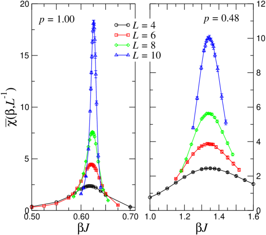
Figure 1: Evolution of the susceptibility as the size of the system increases (up to $L=10$) in the two different regimes: pure system $p=1.0$ on the left plot and high dilution $p=0.48$ on the right plot.

As will be demonstrated below, the tricritical dilution dividing these two regimes is roughly located at $p_{\rm TCP}\approx 0.68-0.84$. In the regime of randomness-induced continuous transitions (or weak first-order transitions, that is at low non-zero bond concentration $p$), the Swendsen-Wang cluster algorithm [22] was preferred in order to reduce the critical slowing-down. As already pointed out by Ballesteros et al. [23, 14], a typical spin configuration at low bond concentration is composed of disconnected clusters for most of the disorder realisations. It is thus safer to use the Swendsen-Wang algorithm, for which the whole lattice is swept at each Monte Carlo iteration, instead of a single-cluster Wolff update procedure. In the strong first-order regime (high bond concentration $p$), the multi-bondic algorithm [24], a multi-canonical version of the Swendsen-Wang algorithm, was chosen in order to enhance tunnellings between the phases in coexistence at the transition temperature. The Swendsen-Wang algorithm, being less time-consuming, was nevertheless preferred even in this regime of long thermal relaxation as long as at least ten tunnelling events between the ordered and disordered phases could be observed. As the first-order regime is approached, more and more sweeps are needed to fulfil this condition. We had to use up to

– $200\ \!000$ Monte Carlo steps (MCS) at $p=0.76$ for $L=16$ for example,

while in the second-order regime for much larger systems, we needed

– $100\ \!000$ MCS at $p=0.68$ for $L=50$,

– $30\ \!000$ MCS at $p=0.56$ for $L=96$, and

– $15\ \!000$ MCS at $p=0.44$ for $L=128$.

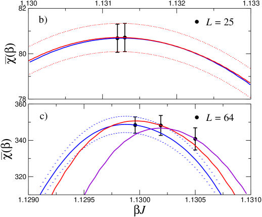
Figure 2: a) Comparison between canonical Swendsen-Wang and multi-bondic algorithms for a pure system ($p=1.0$) of size $L=6$ (histogram reweightings produced from simulations at inverse temperatures $\beta J=0.605$ to $0.655$ are superimposed). The insert shows a zoom of the peak location. b) and c) Histogram reweighting of the average susceptibility $\overline{\chi}(\beta)$ in a disordered system with $p=0.56$ at different sizes $L=25$ and 64. The maximum is progressively obtained after a few iterations (the next simulation is performed at the temperature of the maximum of the histogram reweighting of the current simulation).

This is the essential reason for the size limitation in the first-order regime. A comparison between the two algorithms is illustrated in the case of the pure system for a moderate size ($L=6$) in Fig. 2a. The insert shows a zoom of the peak in the susceptibility and reveals as expected that in this first-order regime, the multi-bondic algorithm provides a better description of the maximum which, since being higher is probably closer to the truth.

In both regimes, the procedure of histogram reweighting enables us to extrapolate thermodynamic quantities to neighbouring temperatures. It leads to a better estimate of the transition temperature and of the maximum of the susceptibility, refining the finite-size estimate at each new size considered, since the maximum is progressively reached (Fig. 2b and 2c). The reweighting has to be done for each sample, then the average is obtained as in Eq. (6). For a particular sample, the probability to measure at a given inverse temperature $\beta$ a microstate $[\sigma]$ with total magnetisation $M_{[\sigma,J]}=M$ and energy $E_{[\sigma,J]}=E$, is $P_{\beta}(M,E)=(Z_{[J]}(\beta))^{-1}\Omega(M,E)\ \!{\rm e}^{\beta E}$ where $\Omega(M,E)$ is the degeneracy of the macrostate. Note that we defined $E$ as minus the energy in order to deal with a positive quantity. We thus get at a different inverse temperature $\beta^{\prime}$

$$P_{\beta^{\prime}}(M,E)=(Z_{[J]}(\beta)/Z_{[J]}(\beta^{\prime}))P_{\beta}(M,E)\ \!{\rm e}^{(\beta^{\prime}-\beta)E},$$ (25)

where the prefactor $(Z_{[J]}(\beta)/Z_{[J]}(\beta^{\prime}))$ only depends on the two temperatures. For any quantity $Q$ depending only on $M_{[\sigma,J]}$ and $E_{[\sigma,J]}$ the thermal average at the new point $\beta^{\prime}$ hence follows from

$$\langle Q_{[J]}\rangle_{\beta^{\prime}}=\frac{\sum_{M,E}Q(M,E)\ \!P_{\beta}(M,E)\ \!{\rm e}^{(\beta^{\prime}-\beta)E}}{\sum_{M,E}P_{\beta}(M,E)\ \!{\rm e}^{(\beta^{\prime}-\beta)E}}.$$ (26)

It is well known that the quality of the reweighting strongly depends on the number of Monte Carlo iterations, the larger this number the better the sampling of the configuration space and thus of the tails of $P_{\beta}$. Here we have to face up to the disorder average also and a compromise between a good disorder statistics and a large temperature scale for the reweighting of individual samples has to be found, but we are mainly interested in the close neighbourhood of the susceptibility maximum, i.e., in a small temperature window.

3.2 Equilibration of the samples and thermal averages

Before any measurement, each sample has to be in thermal equilibrium at the simulation temperature. Starting from an arbitrary initial configuration of spins, during the initial steps of the simulation process, the system explores configurations which are still strongly correlated to the starting configuration. The typical time scale over which this “memory effect” takes place is measured by the autocorrelation time. The integrated energy autocorrelation time $\tau^{e}$ (one can define more generally an autocorrelation time for any quantity) is given by

$$\tau_{[J]}^{e}(\beta)=\frac{1}{2\sigma_{e}^{2}}\sum_{i=0}^{I}\frac{1}{N_{\rm MCS}-I}\sum_{j=1}^{N_{\rm MCS}-I}\left(e^{j}_{[J]}e^{j+i}_{[J]}-\langle e_{[J]}\rangle_{\beta}^{2}\right),$$ (27)

where $\sigma_{e}^{2}=\langle e_{[J]}^{2}\rangle_{\beta}-\langle e_{[J]}\rangle_{\beta}^{2}$ is the variance, $e^{j}_{[J]}$ is the value of the energy density at iteration $j$ for the realization $[J]$, and $I$ is a cutoff (as defined, e.g., by Sokal [25]) introduced in order to avoid to run a double sum up to $N_{\rm MCS}$, which would render the estimates very noisy.

Figure 3: Monte Carlo data of the magnetisation for the disorder realization that gave the largest value of $\chi_{[J]}(\beta_{\rm max})$ for $p=0.44$ at lattice size $L=128$, $p=0.56$ ($L=96$) and $p=0.68$ ($L=50$).

Figure 4: Susceptibility for sample $\#1$ for $p=0.44$ and $L=128$. The different curves show the result of histogram reweighting of simulations close to the maximum location after $5\ \!000$, $10\ \!000$, $12\ \!000$, and $15\ \!000$ MCS. We can safely consider that the value at the temperature of the maximum of the average susceptibility (vertical dashed line) is reliable after $15\ \!000$ MCS.

It is worth giving a definition of the errors as computed in this work. There are two different contributions. Assuming the different realizations of disorder as completely independent, one has an error due to randomness on any physical quantity $Q$, defined according to

$$\Delta_{\rm rdm}\overline{Q}=\left(\frac{\overline{Q^{2}}-\overline{Q}^{2}}{N\{J\}}\right)^{1/2}.$$ (28)

To the thermal average for each sample is also attached an error which depends on the autocorrelation time $\tau^{Q}$, such that the total error on a physical quantity is here defined as:

$$\Delta_{\rm tot}\overline{Q}=\left(\Delta^{2}_{\rm rdm}\overline{Q}+\frac{1}{N\{J\}}\frac{2\overline{\tau^{Q}}\ \overline{\sigma_{Q}^{2}}}{N_{\rm MCS}}\right)^{1/2}.$$ (29)

For each disorder realization, the preliminary configurations have to be discarded and one usually considers that after 20 times the autocorrelation time $\tau^{e}$, thermal equilibrium is reached. The measurement process can then start and the thermal average of the physical quantities is considered, in the case of a single sample, as satisfying when measurements were done during typically $10^{2}\times\tau^{e}$. For a quantity $Q$, a satisfactory relative error of the order of

$$\frac{\Delta_{\rm therm.}\overline{Q}}{\sqrt{\overline{\sigma_{Q}^{2}}}}=\sqrt{\frac{2\overline{\tau^{Q}}}{N\{J\}\times N_{\rm MCS}}}\simeq 10^{-2}$$ (30)

indeed requires typically $N\{J\}\times N_{\rm MCS}\simeq 10^{4}\overline{\tau^{Q}}$. Since we also need a large number of disorder realizations in order to minimise $\Delta^{2}_{\rm rdm}\overline{Q}$, typically $N\{J\}\simeq 10^{2}-10^{4}$, each sample requires a “production” process during $N_{\rm MCS}\simeq(10^{0}-10^{2})\overline{\tau^{Q}}$. In this paper, we choose to work at the upper limit with $N_{\rm MCS}>10^{2}\tau^{e}$ (since there is a single dynamics in the algorithm, the time scale is usually measured through the energy autocorrelation time) and $N\{J\}>10^{3}$.

Examples of times series of the magnetisation are shown in Fig. 3 for particular samples (those which contribute the most to the average susceptibility) at the three largest sizes studied at dilutions $p=0.44$, $0.56$, and $0.64$ in the second-order regime. The simulation temperature is extremely close to the transition temperature and tunnelling between ordered and disordered phases guarantees a reliable thermal average.

Another test of thermal equilibration is given by the influence of the number of MCS which are taken into account in the evaluation of thermal averages. An example is shown in Fig. 4 where the histogram reweightings of the susceptibility, as obtained with different MCS $\#$’s, are shown for a typical sample (the first sample, $\#\ \!1$, is in fact supposed to be typical). Although quite different far from the simulation temperature (which is close to the maximum) the different curves are in a satisfying agreement at the temperature $\beta_{\rm max}$ of the maximum of the average susceptibility, shown by a vertical dashed line. The criterion $\#\ \!$MCS $\geq 250\times\tau^{e}$ is safely satisfied for the larger number of iterations.

3.3 Properties of disorder averages

For different samples, corresponding to distinct disorder realizations, the susceptibility $\chi_{[J]}(\beta)$ at thermal equilibrium may have very different values (see Fig. 5 where the running average over the samples is also shown and remains stable after a few hundreds of realizations).

Figure 5: Different values of $\chi_{[J]}(\beta_{\rm max})$ (over the samples) of susceptibility at $p=0.56$, $L=96$ (the simulation is performed at the temperature of the maximum of the average susceptibility). The running average over the samples is shown by the solid line.

We paid attention to average the data over a sufficiently large number of disorder realizations (typically 2000 to 5000) to ensure reliable estimates of non-self-averaging quantities [26]. Averaging over a too small number of random configurations leads to typical (i.e. most probable) values instead of average ones. Indeed, as can be seen in Fig. 6, the probability distribution of $\chi_{[J]}$ (plotted at the temperature $\beta_{\rm max}$ where the average susceptibility is maximum) presents a long tail of rare events with large values of the susceptibility. These samples have a large contribution to the average, shifted far from the most probable value. The larger the value of $p$, the longer the tail. Scanning the regime close to the first-order transition thus requires large numbers of samples to explore efficiently the configuration space, so the simulations were limited to $L=50$ at $p=0.68$ while we made the calculation up to $L=128$ at $p=0.44$. In the example of Fig. 3, the thermodynamic quantities have been averaged over $3500$ disorder realizations for $p=0.44$ at lattice size $L=128$, $2048$ for $p=0.56$, $L=96$, and $5000$ disorder realizations for $p=0.68$, $L=50$.

Figure 6: Probability distribution of the susceptibility $\chi_{[J]}(\beta_{\rm max})$ for the bond concentrations $p=0.44$, $0.56$, and $0.68$ for the largest lattice size in each case. The full curve represents the integrated distribution. At each dilution, a full vertical line shows the location of the average susceptibility, a dashed line shows the median and a dotted line shows the average over the events which are smaller than the median.

Self-averaging properties are quantified through the normalised squared width, for example in the case of the susceptibility, $R_{\chi}=\sigma_{\chi}^{2}(L)/\overline{\chi}^{2}$, where $\sigma_{\chi}^{2}=\overline{\chi^{2}}-\overline{\chi}^{2}$. For a self-averaging quantity, say $Q$, the probability distribution, albeit not truly Gaussian, may be considered so in first approximation close to the peak, and $P_{\beta}(Q)\simeq(2\pi\sigma_{Q}^{2})^{-1/2}{\rm e}^{-(Q-\overline{\langle Q\rangle})^{2}/2\sigma_{Q}^{2}}$ evolves towards a sharp peak in the thermodynamic limit, $P_{\beta}(Q)\to_{L\to\infty}\delta(Q-\overline{\langle Q\rangle})$. The probability of the average event $\overline{\langle Q\rangle}$ goes to 1 and the normalised squared width evolves towards zero in the thermodynamic limit while it keeps a finite value for a non-self-averaging quantity, as shown in the case of the susceptibility in Fig. 7. The observation of a longer tail in the probability distribution of the $\chi$ values when $p$ increases is expressed in Fig. 7 by the fact that $\chi$ becomes less and less self-averaging when $p$ increases.

Figure 7: Normalised squared width of the susceptibility, $R_{\chi}$, plotted against the inverse lattice size for the three dilutions $p=0.44$, 0.56, and 0.68. The solid lines are polynomial fits used as guides for the eyes. Note that $\chi$ is apparently less and less self-averaging as $p$ increases.

Figure 8: Normalised squared width of the energy, $R_{E}$ plotted on a log-log scale against the inverse lattice size for the three dilutions $p=0.44$, 0.56, and 0.68. Power-law fits have been performed and corresponding exponents printed by the curve. The insert presents the same data plotted on a linear scale.

In contradistinction to the magnetic susceptibility, the energy seems to be weakly self-averaging in the range of lattice sizes that we studied as seen in Fig. 8. The associated exponent depends on the concentration of bonds $p$. This concentration dependence may be effective and due to corrections generated by other fixed points (see below).

In Table 1, the influence of the number of MCS is shown for typical samples, but also for the average susceptibility. Although the variations for a given sample and from sample to sample are important, the average seems stable with our choice of number of iterations (the largest), and also the autocorrelation time (for the average) is stable.

Table 1: Evolution of the susceptibility with the number of Monte Carlo sweeps per spin for different samples, $\chi_{[J]}$ and the average value (with 2048 samples) at $p=0.56$, $L=96$. The data are given at the maximum location of the average susceptibility, $\beta_{\rm max}$. The last column gives the number of independent measurements per sample.

$N_{\rm MCS}$	$\chi_{\#1}$	$\chi_{\#2}$	$\chi_{\#3}$	$\chi_{\#4}$	$\chi_{\#5}$	$\overline{\chi}_{\rm max}$	$\tau^{e}(\beta_{\rm max})$	meas. $/$ sample
5000	994	404	611	682	1803	617(8)	95.1	$\simeq\,~{}50$
10000	952	390	698	614	1574	634(8)	107.4	$\simeq\,~{}90$
15000	1010	356	680	819	1398	638(8)	111.7	$\simeq 130$
20000	939	351	689	851	1320	641(7)	114.0	$\simeq 175$
25000	911	327	675	848	1308	643(8)	115.3	$\simeq 200$
30000	934	327	733	837	1297	643(8)	116.9	$\simeq 250$

In Fig. 6, a full vertical line points out the location of the average susceptibility $\overline{\chi}_{\rm max}$. In order to give a comparison, the median value $\chi_{\rm med}$, defined as the value of $\chi_{[J]}$ where the integrated probability takes the value $50\%$, is shown as the dashed line. The more it differs from the average, the more asymmetric is the probability distribution. This is more pronounced when $p$ increases. We also notice that the maximum of the probability distribution (the typical samples) corresponds to smaller susceptibilities. For a given number of disorder realizations, this peak is better described than the tail at larger susceptibilities, so we also define (shown as dotted lines) an average over the samples smaller than the median susceptibility, that we denote $\chi_{50\%}$,

$$\chi_{50\%}=2\int_{0}^{\chi_{\rm med}}\chi_{[J]}P_{\beta}(\chi_{[J]})\ \!{d}\chi_{[J]},\quad\quad\int_{0}^{\chi_{\rm med}}P_{\beta}(\chi_{[J]})\ \!{d}\chi_{[J]}={1\over 2},$$ (31)

where the factor $2$ normalises the truncated distribution. In the particular case of the probability distributions observed here, i.e. with a sharp initial increase, a peak located at small events and a long tail at large values of the variable, this definition empirically gives a sensitive measure of the typical or most probable value. We shall refer to this quantity when typical behaviour will be concerned.

4 Qualitative description of the transition

Before performing a quantitative analysis of the transition, it is interesting to study in some detail why the probability distributions have significantly different shapes when $p$ varies, and which type of sample can be considered as a typical one, or which one corresponds to a rare event with quite a large or very small susceptibility. Here we shall focus on the second-order regime and in particular on $p=0.44$ for the largest simulated size, $L=128$, for which the probability distribution of $\chi_{[J]}$ at $\beta_{\rm max}$ can be inspected in Fig. 6.

Table 2: Relative variations of the peak height $\Delta\chi_{[J]}/\bar{\chi}_{\rm max}$ and peak location $\Delta\beta_{[J],{\rm max}}/\beta_{\rm max}$ for a few samples, chosen among the rare and the typical samples at $p=0.44$, $L=128$. For reference, the values of the average are given by $\beta_{\rm max}J=1.4820$, $\overline{\chi}_{\rm max}=1450$. The asterisks $(*)$ mark those samples that are discussed in detail in Figs. 12 – 14.

type	sample $\#$	$\chi_{[J],{\rm max}}$	$\beta_{[J],{\rm max}}J$	$\Delta\chi_{[J]}/\bar{\chi}_{\rm max}$	$\Delta\beta_{[J],{\rm max}}/\beta_{\rm max}$
	0035 (*)	5253	1.4823	$262.3~{}\%$	$\,~{}~{}0.02~{}\%$
rare	0438	3862	1.4822	$166.3~{}\%$	$\,~{}~{}0.013~{}\%$
(large $\chi$)	1135	3825	1.4821	$163.8~{}\%$	$\,~{}~{}0.007~{}\%$
	3302	4314	1.4823	$197.5~{}\%$	$\,~{}~{}0.02~{}\%$
	0006	1550	1.4831	$6.9~{}\%$	$\,~{}~{}0.07~{}\%$
typical	0008 (*)	2792	1.4810	$92.5~{}\%$	$-0.07~{}\%$
(around peak)	0021	1473	1.4819	$1.6~{}\%$	$-0.007~{}\%$
	0039	2345	1.4817	$61.7~{}\%$	$-0.02~{}\%$
	0373	946	1.4852	$-34.7~{}\%$	$\,~{}~{}0.22~{}\%$
rare	1492 (*)	286	1.4830	$-80.3~{}\%$	$\,~{}~{}0.07~{}\%$
(small $\chi$)	1967	1063	1.4847	$-26.7~{}\%$	$\,~{}~{}0.2~{}\%$
	2294	769	1.4853	$-46.9~{}\%$	$\,~{}~{}0.2~{}\%$

Each sample displays its own maximum and due to the fluctuations over disorder, the temperature $\beta_{[J],{\rm max}}$ where it occurs varies from sample to sample. In Table 2, we quote for a few rare and typical samples the values of $\chi_{[J]_{\rm max}}$ and $\beta_{[J],{\rm max}}$, the maximum of the sample susceptibility and the corresponding inverse temperature (see also Figs. 9 to 11). The relative variations of these numbers with respect to their average values at $\beta_{\rm max}$ : $\Delta\chi_{[J]}/\bar{\chi}_{\rm max}=[\chi_{[J],{\rm max}}-\bar{\chi}_{\rm max}]/\bar{\chi}_{\rm max}$, and $\Delta\beta_{[J]}/\beta_{\rm max}=[\beta_{[J],{\rm max}}-\beta_{\rm max}]/\beta_{\rm max}$ are also collected in Table 2. It turns out that rare events with large susceptibility do also display a very small shift of the temperature $\beta_{[J],{\rm max}}$ with respect to the average. Other events have a smaller susceptibility at $\beta_{\rm max}$ both because their maximum $\chi_{[J],{\rm max}}$ is smaller but also because of a larger shift of the temperature $\beta_{[J],{\rm max}}$ where this maximum occurs. A few examples of rare events corresponding to large values of $\chi_{[J]}$ are shown in Fig. 9. Rare events corresponding to small values of $\chi_{[J]}$ are presented in Fig. 11. They have a very small contribution to the phase transition so in the following, we will refer only to events with large values of $\chi_{[J]}$ when mentioning rare events. In Fig. 10, the same is done for typical events, i.e., those for which the values of $\chi_{[J]}$ are in the peak of the distribution. The scales of both axis are the same in the three figures in order to facilitate the comparison.

Figure 9: Examples of rare events for $p=0.44$ and $L=128$. with large values of $\chi_{[J]}$. The thick lines show the averages over all realizations.

Figure 10: Examples of typical events for the same parameters as in Fig. 9. The thick lines show the averages over all realizations.

Figure 11: Examples of rare events for the same parameters as in Fig. 9 with $\chi_{[J]}$ at the foot of the probability distribution. The thick lines show the averages over all realizations.

Figure 12: Time series of the magnetisation and the energy density and corresponding probability distributions for a rare event ($\#35$) with large $\chi_{[J]}$ ($p=0.44$, $L=128$, simulation at inverse temperature $\beta J=1.48218$).

Figure 13: Time series of the magnetisation and the energy density and corresponding probability distributions for a typical event ($\#8$) with $\chi_{[J]}$ in the vicinity of the most probable value ($p=0.44$, $L=128$, simulation at inverse temperature $\beta J=1.48218$).

Figure 14: Time series of the magnetisation and the energy density and corresponding probability distributions for a rare event ($\#1492$) with very small $\chi_{[J]}$, which looks similar to typical events ($p=0.44$, $L=128$, simulation at inverse temperature $\beta J=1.48218$).

In Figs. 12-14, we can follow the fluctuations of the magnetisation during the thermalisation process (after equilibration) for three different samples. Configuration $\#35$ (Fig. 12) corresponds to a rare event, with the definition given above, while the sample $\#8$ (Fig. 13) is a typical one. The last sample, $\#1492$ (Fig. 14), is an example of a realization of disorder which leads to a very small susceptibility peak. These figures also present the magnetisation and energy probability distributions. The rare event (Fig. 12) displays a double-peak structure in the probability distributions (only a shoulder is visible in $P_{\beta_{\rm max}}(e_{[J]})$), presumably a remnant of the first-order type transition of the pure system. In the average behaviour, it seems that at small values of $p$, these types of samples are “lost” in the large majority of typical samples which have a “second-order type” of probability distribution. This observation is corroborated by similar “signals” in Figs. 9 to 11 concerning the shape of the susceptibility (narrow peak for rare events with large susceptibilities and broader for others), of the order parameter (sharp increase with $\beta$ at the transition for rare events, and smoother variation for the typical samples), or of the Binder cumulant (deep well at the transition in the case of rare events and less pronounced wells for typical ones).

Figure 15: Probability distribution of the susceptibility for a system of size $L=20$ at $p=0.84$ and $\beta J=0.74704$, in the seemingly first-order regime. The simulation was performed with the multibondic algorithm.

Figure 16: Probability distributions $\overline{P}$ and $P_{[J]}$ of the energy $e$ for the average behaviour and for a rare event (large susceptibility), respectively, at $p=0.84$ ($L=13$). The double-peak structure suggests a behaviour for this specific sample which is similar to the one observed at a first-order transition. The simulation is performed at inverse temperature $\beta J=0.746\,356$.

We may thus argue that a possible mechanism which keeps the pure model’s first-order character of the transition at larger values of $p$ is connected to the occurrence of a larger proportion of samples with the “first-order type”, i.e., a very big susceptibility signal at $\beta_{\rm max}$. In Fig. 15, the quite long tail of large susceptibilities in the susceptibility distribution confirms this assumption, for $p=0.84$ ($L=20$), i.e., closer to, or probably inside the first-order regime. Also the double-peak structure of the energy distribution at this dilution (see Fig. 16) is compatible with a first-order like transition for the average behaviour (of course one would have to study the evolution of the energy barrier as the size increases, but this makes no sense for a specific disorder realization for which the notion of thermodynamic limit is meaningless). The possible interpretation is that the rare events of higher susceptibilities when $p$ becomes larger are more comparable to a system displaying a first-order transition. This would explain that the susceptibility peak is narrower (and thus does coincide with the temperature of the maximum of the average only in very rare cases).

5 Phase diagram and strength of the transition

5.1 Transition line

We can now come back to the preliminary phases of this work. The transition temperature was determined for 19 values of the bond concentration ranging from $p=0.28$ to $p=1.00$ (pure system). We defined an effective inverse transition temperature $\beta_{c}(L,p)$ at a given lattice size $L$ as the location of the maximum of the average magnetic susceptibility $\overline{\chi}$ (see Fig. 17). Any diverging quantity could equally have been chosen but it turned out that the specific heat was displaying larger statistical errors than the magnetic susceptibility. Moreover, the stability of the random fixed point implies a slowly varying specific heat with a critical exponent $\alpha\leq 0$.

For each $p$ and $L$, several Monte Carlo simulations were necessary to get a reasonable estimate of $\beta_{c}(L,p)$. As mentioned before, histogram reweighting was used to refine the determination. The procedure was applied up to lattice sizes $L=16$. The resulting phase diagram for two different lattice sizes is plotted in Fig. 18. The data appear to be in a remarkable accordance.

The numerical data presented in Fig. 18 are furthermore in agreement with the mean-field prediction $T_{c}(p)=pT_{c}(p=1)$ for large bond concentration, close to the pure system ($p\simeq 1$). At smaller concentration $p$, the topological properties of the bond configuration become important and the mean-field prediction fails to reproduce the observed behaviour. The effective-medium approximation introduced in this context in the eighties

Figure 17: Average susceptibility and its histogram reweighting for systems of sizes $10^{3}$ and $16^{3}$ for dilutions (from left to right) $p=0.32$, 0.40, 0.48, 0.56, 0.64, 0.72, 0.80, 0.88, and 0.96.

by Turban [28] reproduces quite accurately the numerical data. Limiting the approximation to a single bond, the following estimate for the transition temperature is obtained:

$$\beta_{c}(p)=J^{-1}\ln\left[{(1-p_{c})e^{\beta_{c}^{\rm pure}J}-(1-p)\over(p-p_{c})}\right],$$ (32)

where $\beta_{c}^{\rm pure}J=0.62863(2)$ for the pure system. This expression is exact (as exact as it might be with numerical factors introduced) in the limits of the pure system ($p=1$) and the percolation threshold ($p_{c}=0.248\,812\,6(5)$).

Figure 18: Transition temperatures $k_{B}T_{c}(p)/J$ with respect to the bond concentration $p$ for two lattice sizes $L=10$ and $L=16$. Mean-field and effective-medium approximations are also indicated by the dashed and solid lines, respectively.

5.2 Order of the transition

Distinguishing a weak first-order phase transition from a continuous one is a very difficult task. The autocorrelation time of the energy $\tau^{e}$ at the transition temperature may be useful, since it displays a behaviour which depends on the order of the transition. When using a canonical Monte Carlo simulation for the study of a first-order transition, the time-scale of the dynamics is dominated by the tunnelling events between the ordered and disordered phases in coexistence at the transition temperature. Such a tunnelling event implies the creation and the growth of an interface whose energy cost behaves as $\beta\Delta F=2\sigma_{\rm o.d.}L^{D-1}$ where $\sigma_{\rm o.d.}$ is the reduced interface tension. As a consequence, the autocorrelation time grows exponentially as

$$\tau^{e}(L)\sim e^{{2\sigma_{\rm o.d.}}L^{D-1}}.$$ (33)

For a continuous phase transition, this interface tension vanishes and the autocorrelation time scales as a power-law of the lattice size,

$$\tau^{e}(L)\sim L^{z},$$ (34)

where $z$ is the dynamical critical exponent.

Figure 19: Autocorrelation time of the energy $\tau^{e}$ with respect to the lattice size at the (pseudo-) transition temperature. The curves correspond to different bond concentrations $p$ (from bottom $p=0.28$ to the top $p=1.00$ in steps of $0.04$). The results shown here all follow from MC simulations using the Swendsen-Wang algorithm.

The numerical estimates of the autocorrelation time $\tau^{e}$ are plotted in Fig. 19 for several dilutions. They show a growth of the autocorrelation time with the lattice size which becomes dramatic as the bond concentration increases and a behaviour compatible with a power law of the system size when $p$ decreases, as expected since the dilution softens the transition and thus reduces the dynamical exponent $z$. Nevertheless, it is not possible to distinguish precisely the two regimes on a plot of the autocorrelation time versus the lattice size. Here, we may locate approximately the boundary between the two regimes around – slightly above $p=0.68$. Indeed, the autocorrelation time at $p=0.68$ is very well fitted with a power-law for all lattice sizes smaller than $L=30$. Above, the data display a downward bending that can be explained by a correction to the power-law behaviour but not by an exponential prefactor (the bending would be upward). On the other hand, for $p=0.84$ it is not possible to find any set of three consecutive points that could be fitted by a power-law: the autocorrelation time clearly grows faster than a power-law. Using two successive lattice sizes $L_{1}$ and $L_{2}>L_{1}$, we defined an effective dynamical exponent

$$z_{\rm eff}(L_{1},L_{2})={\ln\tau^{e}(L_{2})-\ln\tau^{e}(L_{1})\over\ln L_{2}-\ln L_{1}}$$ (35)

which is expected to reach a finite value for continuous transitions and to diverge for first-order ones. The data, plotted in Fig. 20, again do not lead to any sound estimate of the location of the tricritical point. Nevertheless, the transition again definitely remains continuous up to the bond concentration $p=0.68$. For higher concentrations, the data show an increase of the dynamical exponent with lattice size, but it is not possible to state unambiguously whether they develop a divergence or not. We also notice that the necessary finite number of iterations leads to an underestimate of $\tau^{e}$ and thus of $z$ for bond concentrations close to $p=1$ at large lattice sizes (this is particularly clear in Fig. 20 for the size $L=13-16$). Multi-bondic simulations were thus needed in this case to improve the measurement of thermodynamic quantities when $p$ is close to 1.

Figure 20: Effective dynamical exponent (SW algorithm) with respect to the smaller lattice size at the transition temperature. The curves correspond to different bond concentrations $p$ (from bottom $p=0.28$ to the top $p=1.00$ in steps of $0.04$).

Figure 21: Probability distribution of the energy at the temperature for which the two peaks have equal heights. The two plots correspond to two different bond concentrations: $p=0.56$ on the left (SW algorithm, increasing sizes $L=25$, 30, 35, 40, 50, 64, and 96) and $p=0.84$ on the right (multi-bondic simulations, sizes $L=16$, 20, and 25). The order-disorder interface tension $\sigma_{\rm o.d.}=\ln(P_{\rm max}/P_{\rm min})/(2L^{D-1})$ is plotted against $L^{-1}$ in the upper part of the figure.

Another approach is provided by the behaviour of the order-disorder interface tension. Numerically, the interface tension can be estimated from the probability distribution $P(e)$ of the energy. One has

$${P_{\rm min}\over P_{\rm max}}\propto e^{-{\beta\Delta F}}=e^{-2\sigma_{\rm o.d.}L^{D-1}}.$$ (36)

Indeed, the free-energy barrier can be related to the ratio of the (equally high) probabilities of the ordered and disordered phases (corresponding to the two peaks) and of the mixed phase regime involving two interfaces and which corresponds to the bottom of the gap between the two peaks. We started from the effective transition temperatures estimated from the maxima of the magnetic susceptibility. At this temperature, the statistical weight of the ordered and disordered phases are comparable so the height of the peaks is very different. In order to define the interface tension, we reweighted the time series of the simulations to the (close) temperature for which the two peaks have equal heights. The order-disorder interface tension is plotted against the inverse of the lattice size at the transition temperature in the upper part of Fig. 21. It shows undoubtedly a vanishing of the interface tension for $p=0.56$, and presumably for $p=0.76$ (not shown here) also, being a clear indication of a disorder induced second-order transition. On the other hand, for $p=0.84$ the interface tension seems to converge towards a finite (but very small?) value in the thermodynamic limit, which can be taken as a signal for the persistence of the first-order nature of the transition in the pure case at $p=1$ down to this dilution.

As a consequence, we are led to the conclusion that the tricritical point is presumably located between $p=0.68$ and $p=0.84$, the upper bound corresponding to the observation of an exponential growth of the autocorrelation time and the lower to a constant dynamical exponent and the vanishing of the latent heat (both values of $p$ are indicated in the previous Figs. 19 and 20). However, one cannot unambiguously prove by numerical simulations on finite systems that what we identified as a second-order phase transition is not a weak first-order phase transition with a correlation length larger than $L=128$, or that the fast growth of the autocorrelation time for $p\geq 0.84$ is not a cross-over to a power-law regime at larger system sizes.

6 Critical behaviour

6.1 Leading behaviour and critical exponents

We now concentrate on the second-order regime only, i.e., on $p\leq 0.68$ where we performed an investigation of the universality class at the disorder fixed point. The critical exponents are computed using the finite-size scaling behaviour of the physical quantities (Eqs. (14)-(17)) at the effective transition temperature $\beta_{c}(L,p)$. In the usual renormalisation group scheme for disordered systems, the renormalisation flow is subject to the influence of three fixed points describing respectively the pure system, the random system and the percolation transition. The scaling behaviour is thus expected to display large corrections resulting in a cross-over to a unique universal behaviour at large lattice sizes. According to this scheme, the exponents which are measured are expected to be (apparently) concentration dependent. In the previous sections (see, e.g., Fig. 17), the corrections to scaling for the transition temperature have been observed to be weaker for the bond concentration $p=0.56$. This behaviour is illustrated, e.g., in Fig. 22 where the cross-over effect reflects in the bending of the curves $\beta_{\rm max}(L,p)J$ vs. $L^{-1}$ for three dilutions $p=0.32$, $p=0.56$, and $p=0.80$. The curve at $p=0.56$, on the other hand, is almost flat. The corresponding data for the three main dilutions in the second order regime, $p=0.44$, $p=0.56$, and $p=0.68$, are then plotted against $L^{-1/\nu}$ on the right part. Although the value of $\nu$ is not yet known, we anticipate here the later result, using already the “to-be-determined-exponent”. Again, the curve at $p=0.56$ has an almost vanishing slope. As a consequence, we decided to make further large-scale Monte Carlo simulations at this concentration $p=0.56$ up to the lattice size $L=96$. To monitor the effects of the competing fixed points, we also made additional large-scale simulations for the concentrations $p=0.44$ (towards the percolation transition) and $p=0.68$ (towards the regime of first-order transitions) up to the lattice sizes $L=128$ and $L=50$, respectively (size limitations at these concentrations are linked to the discussion of Sect. 3).

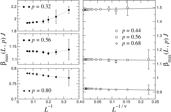
Figure 22: Evolution of the size-dependent (pseudo-)critical coupling with the inverse system size for relatively small sizes on the left plots. The same on the right plot for the three main dilutions, where the data are by anticipation fitted to a linear relation $\beta_{\rm max}(L,p)=\beta_{c}(p)+aL^{-1/\nu}+\dots$, where our estimate for $\nu$ ($\approx 0.75$) will be discussed later. The slope coefficient is slightly positive for $p=0.44$, slightly negative for $p=0.68$ and virtually zero at $p=0.56$, where the corrections-to-scaling (at least for this quantity) appear to be the smallest.

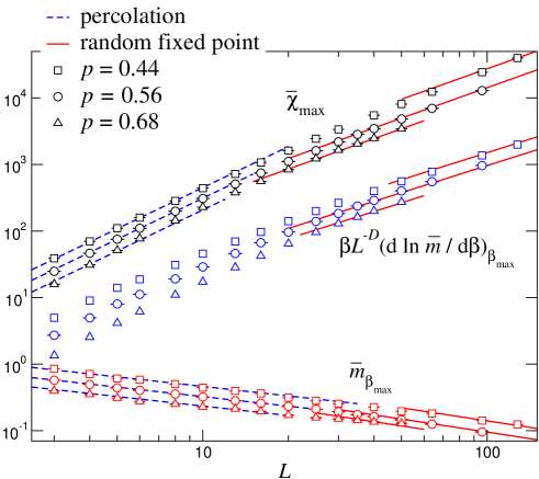
Figure 23: Finite-size scaling behaviour of the susceptibility, the magnetisation and of $\beta L^{-D}d\ln\overline{m}/d\beta$ at $\beta_{\rm max}$ (the quantities have been shifted in the vertical direction for the sake of clarity). The behaviour at small lattice sizes is presumably governed by the percolation fixed point (shown as dashed lines and characterised by exponent ratios $\gamma/\nu\simeq 2.05$ and $\beta/\nu\simeq 0.475$). Above a crossover length scale a new (random) fixed point is reached (shown by the solid lines, with exponent ratios $\gamma/\nu\simeq 1.535$, $1/\nu\simeq 1.34$, and $\beta/\nu\simeq 0.73$, discussed in detail below).

Figure 24: Log-log plot of the average susceptibility (open symbols) and the typical susceptibility (filled symbols), as defined in Eq. (31) by $\chi_{50\%}$ for the three principal dilutions studied, indicating that the asymptotic scaling regime sets in earlier for the latter quantity.

In Fig. 23, the finite-size scaling behaviour of the maximum susceptibility, $\overline{\chi}_{\rm max}$, the magnetisation at $\beta_{\rm max}$ and the derivative of $\ln\overline{m}$ with respect to the inverse temperature evaluated at ${\beta_{\rm max}}$ are plotted versus the system size on a log-log scale. These curves should give access to the exponents $\gamma/\nu$, $\beta/\nu$, and $1/\nu$, respectively. The three main dilutions are represented. One clearly observes a crossover between two regimes. For small lattice sizes, the system is strongly influenced by the proximity of a perturbing fixed point while a different, unique fixed point, is apparently reached at large sizes, as revealed by the slopes which are at first sight independent of the dilution when the linear extent of the lattice reaches values of about $L\geq 30$. The most probable susceptibility $\chi_{50\%}$ is shown in Fig. 24 and can also lead to estimates for $\gamma/\nu$. According to the discussion given in Sect. 3, we expect that the most probable susceptibility is better described than the average susceptibility, for which there exists a significant contribution of rare events, and these rare disorder realizations might be poorly scanned if a too small number of samples is considered. This difficulty might be circumvented through the study of what we defined as $\chi_{50\%}$ in Eq. (31). In the presence of multifractality, the universal behaviour of $\chi_{50\%}$ should differ from that of $\overline{\chi}$. Since such a peculiar behaviour does not occur in the case of a global quantity [26], like $\chi$, we expect compatible values of $\gamma/\nu$ as deduced from $\chi_{50\%}$ or $\overline{\chi}$. Observing the data plotted in Fig. 24, in fact, confirms our previous analysis. It seems that $\chi_{50\%}$ is less influenced by the crossover effects than the average $\overline{\chi}_{\rm max}$. In order to support this statement, we will present the results of fits of the susceptibility in two different tables for the two regimes and for the three main dilutions:

• At small lattice sizes, the behaviour of $\overline{\chi}_{\rm max}$ and $\overline{m}_{\beta_{\rm max}}$ is in all three cases compatible with the percolation exponents $(\gamma/\nu)_{\rm perco}\simeq 2.05$ and $(\beta/\nu)_{\rm perco}\simeq 0.475$ shown in Fig. 23 by the dashed lines. This seems to be true (particularly in the case of the susceptibility) over a wider range of sizes for $p=0.44$ than for $p=0.56$ or $p=0.68$. This observation is compatible with a stronger influence of the percolation fixed point when $p=0.44$, which is closer to the percolation threshold than the two other dilutions. Surprisingly, the assumption of a percolation influence is absolutely not confirmed by the behaviour at small sizes of the third quantity of interest, $L^{-D}(d\ln\overline{m}/d\beta)_{\beta_{\rm max}}$. Due to the involved differentiation with respect to inverse temperature, the identification with percolation quantities becomes less obvious, but we do not have any explanation for this strange result. In Table 3, we try to point out the influence of the percolation fixed point. This is achieved by power-law fits between a fixed minimum size $L_{\rm min}=4$ up to an increasing maximum size $L_{\rm max}$ below the value $L=30$ which apparently marks the modification in the behaviour of the physical quantities under interest. We first observe that $\beta/\nu$ starts from a value very close to the percolation value, and second, that $\chi_{50\%}$ has always a lower exponent (i.e. more distinct from the percolation value).

  Table 3: Exponents deduced from the finite-size scaling behaviour of $\overline{\chi}_{\rm max}$ and $\chi_{50\%}$ in the vicinity of the percolation fixed point (small sizes). Recall the percolation value $(\gamma/\nu)_{\rm perco}\simeq 2.05$ for comparison.

  		$p=0.44$		$p=0.56$		$p=0.68$
  		$\gamma/\nu$ deduced from		$\gamma/\nu$ deduced from		$\gamma/\nu$ deduced from
  $L_{\rm min}$	$L_{\rm max}$	$\overline{\chi}_{\rm max}$	$\chi_{50\%}$	$\overline{\chi}_{\rm max}$	$\chi_{50\%}$	$\overline{\chi}_{\rm max}$	$\chi_{50\%}$
  4	8	2.015	1.902	2.098	1.916	2.211	1.915
  4	13	1.984	1.866	2.034	1.818	2.132	1.720
  4	20	1.954	1.833	1.973	1.748	2.051	1.579
  4	30	1.924	1.808	1.913	1.691	1.974	1.500

  Table 4: Exponents deduced from the finite-size scaling behaviour of $\overline{\chi}_{\rm max}$ and $\chi_{50\%}$ in the vicinity of the random fixed point (large sizes). The largest size taken into account in the fits is $L_{\rm max}=128$ for $p=0.44$, 96 for $p=0.56$, and 50 for $p=0.68$.

  	$p=0.44$		$p=0.56$		$p=0.68$
  	$\gamma/\nu$ deduced from		$\gamma/\nu$ deduced from		$\gamma/\nu$ deduced from
  $L_{\rm min}$	$\overline{\chi}_{\rm max}$	$\chi_{50\%}$	$\overline{\chi}_{\rm max}$	$\chi_{50\%}$	$\overline{\chi}_{\rm max}$	$\chi_{50\%}$
  20	1.724	1.672	1.571	1.579	1.541	1.412
  25	1.711	1.664	1.543	1.587	1.479	1.471
  30	1.706	1.669	1.518	1.596	1.438	1.539
  35	-	-	1.500	1.581	1.447	1.645
  40	1.703	1.679	1.502	1.587	1.464	1.675
  50	1.695	1.657	1.506	1.593
  64	1.680	1.659

• At large sizes, for each quantity considered here, the curves corresponding to the three dilutions in Figs. 23 and 24 evolve, after a crossover regime whose exact location depends on the value of $p$, towards a presumably unique power-law behaviour which seems to remain stable then (solid lines in Fig. 23). We thus believe that we have reached large enough sizes in order to get reliable estimates of the random fixed point exponents. This is only a visual impression, since in fact the effective exponents are still subject to significant variations, especially for the extreme dilutions $p=0.44$ and $p=0.68$. Effective exponents $\gamma/\nu$, $\beta/\nu$, and $1/\nu$ may be defined from power-law fits of $\overline{\chi}_{\rm max}$, $\overline{m}_{\beta_{\rm max}}$, and $L^{-D}d\ln\overline{m}/d\beta$ between an increasing minimum size, $L_{\rm min}$, and a maximum one, $L_{\rm max}$. The value $L_{\max}$ is kept to the maximum available value $L=128$, $96$, and $50$ for $p=0.44$, 0.56, and 0.68, respectively, and the results for the susceptibility are presented in Table 4. We see there that $\chi_{50\%}$ is again better behaved (more stable) than the average susceptibility.

Since we are mainly interested in the randomness fixed point, we now concentrate on fits at large system sizes. An exhaustive summary (i.e. for all three dilutions under interest) of the results of the fits performed at dilutions $p=0.44$, $p=0.56$, and $p=0.68$ is presented in Table 5. The corresponding effective exponents are also plotted against $L^{-1}_{\rm min}$ in Fig. 25. These results show that the data analysis is much more complicated than our previous preliminary determination of exponents in Table 4. Again, the crossover between percolation and random fixed point behaviours is visible through the variation of effective exponents and the data present large corrections-to-scaling.

Table 5: Linear fits for $\overline{\chi}_{\rm max}$, $\overline{m}_{\beta_{\rm max}}$, and $L^{-D}d\ln\overline{m}/d\beta$ at $\beta_{\rm max}$, leading to finite-size estimates of the combinations of critical exponents $\gamma/\nu$, $\beta/\nu$ and $1/\nu$. These results correspond to the three main dilutions, and they are extracted from the finite-size scaling behaviour of the quantities at the temperature where the maximum of the average susceptibility is found by histogram reweighting. The results for dilutions $p=0.44$ and $p=0.68$ are less stable than for $p=0.56$, reflecting the role of the crossover.

$p$	$L_{\rm min}$	$L_{\rm max}$	$\gamma/\nu$	error	$\beta/\nu$	error	$1/\nu$	error	$\gamma/\nu+2\beta/\nu$
0.44	30	128	1.706	0.006	0.544	0.005	1.395	0.006	2.794(16)
—	40	—	1.703	0.008	0.552	0.007	1.381	0.008	2.807(22)
—	50	—	1.695	0.010	0.540	0.009	1.358	0.010	2.775(28)
—	64	—	1.680	0.016	0.534	0.014	1.357	0.016	2.748(44)
0.56	30	96	1.518	0.011	0.588	0.010	1.389	0.011	2.694(31)
—	35	—	1.500	0.014	0.592	0.012	1.362	0.013	2.684(38)
—	40	—	1.502	0.016	0.608	0.015	1.353	0.016	2.718(46)
—	50	—	1.506	0.026	0.645	0.024	1.330	0.025	2.796(74)
0.68	25	64	1.479	0.021	0.343	0.015	1.505	0.021	2.165(51)
—	30	—	1.438	0.031	0.344	0.022	1.453	0.030	2.126(75)
—	35	—	1.447	0.047	0.342	0.033	1.437	0.046	2.13(11)
—	40	—	1.464	0.075	0.547	0.051	1.379	0.075	2.56(18)

Figure 25: Effective critical exponents $\gamma/\nu$ and $\beta/\nu$, as computed from a power-law fit between $L_{\rm min}$ and $L_{\rm max}$, with $L_{\max}$ fixed to the maximum available value $L=128$, $96$ and $50$ for $p=0.44$, 0.56, and 0.68, respectively. They are plotted against $L^{-1}_{\rm min}$. The thin solid line shows the percolation values and the shadow stripe corresponds to our estimate for the random fixed point values. In the case of the dilution $p=0.56$, the value of $2\beta/\nu+\gamma/\nu$ is also shown.

A precise determination of the magnetic exponents is quite difficult. Indeed, as can be seen in Fig. 25, the effective critical exponents $(\gamma/\nu)_{\rm eff}$ and $(\beta/\nu)_{\rm eff}$ do not converge towards $p$-independent limits when $L_{\rm min}\rightarrow L_{\rm max}$. The cross-over effects on the thermal quantities are much smaller. Indeed, the effective critical exponent $\nu_{\rm eff}$ is converging to a roughly $p$-independent limit when $L_{\rm min}\rightarrow L_{\rm max}$. We can give the following estimates for $\gamma/\nu$ and $1/\nu$ :

$$p=0.44: (\gamma/\nu)_{\rm eff}\simeq 1.68(2), (1/\nu)_{\rm eff}\simeq 1.36(2),$$ (37)

$$p=0.56: (\gamma/\nu)_{\rm eff}\simeq 1.51(3), (1/\nu)_{\rm eff}\simeq 1.33(3),$$ (38)

$$p=0.68: (\gamma/\nu)_{\rm eff}\simeq 1.46(8), (1/\nu)_{\rm eff}\simeq 1.38(8),$$ (39)

simply corresponding to the last line of Table 5, i.e., to the largest studied value of $L_{\rm min}$, for each dilution. The value of $\beta/\nu$ on the other hand is definitely not stable and more subject to the competing influence of fixed points. For $p=0.44$ for example, the estimate of $(\beta/\nu)_{\rm eff}$ is relatively stable against variations of $L_{\rm min}$, with fitted values below $0.5$, close to the expected value for the percolation transition ($0.475$). This is a quantitative indication that the system is probably still subject to cross-over caused by the percolation fixed point. In the case of $p=0.68$, the estimate of $(\beta/\nu)_{\rm eff}$ is very small, then suddenly increasing for $L_{\rm min}=64$. These remarks are consistent with the renormalisation scheme described above. In order to help us to decide between the different effective values measured at the three dilutions, we use the scaling relation $\gamma/\nu+2\beta/\nu=D=3$ which is almost satisfied for the bond concentration $p=0.56$ only (shown in Fig. 25) when taking into account the lattice sizes $L\geq 50$. For the bond concentrations $p=0.44$ and $p=0.68$, this scaling relation is not satisfied for any of the accessible values. One is thus led to conclude that the critical regime has not yet been reached for these concentrations, in spite of our efforts to go up to very large sizes. Remember also that the corrections-to-scaling were found to be the smallest at $p=0.56$, so the asymptotic regime in neighbouring dilutions should be more difficult to reach. Figure 25 thus suggests to rely only on the values measured at dilution $p=0.56$, extrapolated to $L_{\rm min}\to\infty$, as shown in Fig. 26, where a dashed stripe emphasises such an extrapolation of the effective exponents measured at the largest sizes. The values of $(\gamma/\nu)_{\rm eff}$ and $(1/\nu)_{\rm eff}$ are indeed stable in the regime $L\geq 35$. We may thus have reliable estimates of the asymptotic values for these exponents, and a reasonable estimate for $\beta/\nu$, ratifying the scaling relation.

Using this extrapolation procedure, our final estimates of the critical exponents of the disorder induced random fixed point of the three-dimensional bond-diluted 4-state Potts model are the following values:

$$\gamma/\nu =1.535(30),$$ (40)

$$\beta/\nu =0.732(24),$$ (41)

$$1/\nu =1.339(25),$$ (42)

resulting from a linear extrapolation of the data points for $L_{\rm min}=25$, 30, 35, 40, 50, and 64 at $p=0.56$. Note that since the data are correlated, we have kept the error of the last point.

Figure 26: Effective critical exponents $\gamma/\nu$, $\beta/\nu$, and $1/\nu$ for the dilution $p=0.56$ obtained from fits between $L_{\rm min}$ and $L_{\rm max}=96$ and extrapolated to $L_{\rm min}\to\infty$. In this limit, the scaling relation $\gamma/\nu+2\beta/\nu=D$ is nicely satisfied.

6.2 Corrections to scaling

For the 3D disordered Ising model it is well known that the correction-to-scaling close to the random fixed point are strong (with a corrections-to-scaling exponent around $\omega=0.4$). Let us assume here also the existence of an irrelevant scaling field $g$ with scaling dimension $y_{g}=-\omega<0$. The scaling expression for the susceptibility

$$\overline{\chi}(L^{-1},\beta-\beta_{c},g)=L^{\gamma/\nu}f_{\chi}(L|\beta-\beta_{c}|^{\nu},L^{-\omega}g),$$ (43)

expanded at $\beta_{c}$ (on a finite system the susceptibility is always finite) around the fixed point value $g=0$, leads to the standard expression $\Gamma_{c}L^{\gamma/\nu}[1+b_{\chi}L^{-\omega}+O(L^{-2\omega})]$. In order to investigate this question for the 3D 4-state Potts model, we tried to fit the physical quantities for $p=0.56$ as

$$\overline{\chi}_{\rm max}(L)=\Gamma_{c}L^{\gamma/\nu}(1+b_{\chi}L^{-\omega}),$$ (44)

and similar expressions for $\overline{m}_{\beta_{\rm max}}$, in the range $L\geq 25$ where the leading term was already fitted in the previous section, and the subleading correction is due to the first irrelevant scaling field.

Since four-parameter non-linear fits are not stable, we preferred linear fits where the exponents are taken as fixed parameters but the amplitudes are free. In Fig. 27, we show a 3D plot of the cumulated square deviation of the least-square linear fit, $\chi^{2}$, as a function of $\gamma/\nu$ and $\omega$. There is a clear valley which confirms that $\gamma/\nu$ is close to 1.5, but the valley is so

Figure 27: Plot of the $\chi^{2}$ deduced from linear fits of $\overline{\chi}_{\rm max}(L)=\Gamma_{c}L^{\gamma/\nu}(1+b_{\chi}L^{-\omega})$ in the range $25\leq L\leq 96$ for $p=0.56$. The exponents are treated as fixed parameters and the amplitudes are free. The base plane gives the ranges of variation of the exponents: $1.25\leq\gamma/\nu\leq 1.75$ and $0\leq\omega\leq 5$. The absolute minimum is at $\gamma/\nu=1.49$, $\omega=3.88$, but the valley is extremely flat in the $\omega$-direction. A cutoff at $\chi^{2}=50$ has been introduced in order to improve clarity of the figure.

flat in the $\omega$-direction that there is no clear minimum to give a reliable estimation of the corrections-to-scaling exponent. The same procedure for $\beta/\nu$ is illustrated in the next figure (Fig. 28). Again, there is no way to get a compatible corrections-to-scaling exponent from the three fits, but the leading exponents are indeed close to $\beta/\nu=0.71$ (and $1/\nu=1.35$). Of course the minima of $\chi^{2}$ do not exactly coincide with the data presented in the table which should correspond to $\omega\to\infty$.

Figure 28: Plot of the $\chi^{2}$ deduced from linear fits of $\overline{m}$ (the exponent is thus negative) in the range $25\leq L\leq 96$ for $p=0.56$. In the base plane, the range of variation of the exponents is $-1\leq-\beta/\nu\leq-0.5$ and $0\leq\omega\leq 5$, and the minimum is at $\beta/\nu=0.85$, $\omega=0.135$.

7 Conclusion

We studied the three-dimensional bond-diluted 4-state Potts model by large-scale Monte Carlo simulations. The pure system undergoes a strong first-order phase transition. The numerical estimates of the dynamical exponent $z$ and of the interface tension give evidences for the existence of a disorder-induced tricritical point for bond dilutions between $p=0.68$ and $p=0.84$ below which the transition is softened to second order. Very strong crossover corrections are observed up to lattice size $L\leq 30-40$. The regime of the random fixed point is best observed for the bond concentration $p=0.56$. From the values of the ratios of exponents measured at that concentration,

$$\gamma/\nu =1.535(30),$$ (45)

$$\beta/\nu =0.732(24),$$ (46)

$$1/\nu =1.339(25),$$ (47)

the following estimates of the critical exponents are derived:

$$\gamma =1.146(44),$$ (48)

$$\beta =0.547(28),$$ (49)

$$\nu =0.747(14).$$ (50)

Let us mention that these exponents are in reasonably good agreement with recent star-graph high-temperature expansions [16] of this model which give $\gamma=1.00(3)$. The value of $\nu$ is eventually safe with respect to the bound $\nu\geq 2/D=0.6666\dots$ of the stability of the random fixed point. In the random fixed point regime, we are unable to extract from the numerical data any reliable correction-to-scaling exponent (linked to the possible appearance of irrelevant scaling fields), even though it is clear that such corrections cannot be ignored.

In some sense, the outcome of this time-consuming work is disappointing, since we were not able to reach the asymptotic regime where exponents in the second-order regime of the phase diagram become dilution-independent, since the corrections to scaling are too strong, and since the tricritical point was not located with precision. We believe that this is due to the extreme difficulty of the problem and not to an unadapted approach. Perhaps we were too ambitious, but we have the feeling that the final values given for the critical exponents are reliable enough and should not be contradicted in the future by similar studies.

References

- [1] D.E. Khmel’nitskiĭ, Sov. Phys. JETP 41, 981 (1974).
- [2] A.B. Harris, J. Phys. C 7, 1671 (1974).
- [3] A.W.W. Ludwig and J.L. Cardy, Nucl. Phys. B 330 [FS19], 687 (1987); Vl. Dotsenko, M. Picco, and P. Pujol, Nucl. Phys. B 455 [FS], 701 (1995); J.L. Jacobsen and J.L. Cardy, Nucl. Phys. B 515, 701 (1998); T. Olson and A.P. Young, Phys. Rev. B 60, 3428 (1999); C. Chatelain and B. Berche, Nucl. Phys. B 572, 626 (2000); C. Chatelain, B. Berche, and L.N. Shchur, J. Phys. A 34, 9593 (2001).
- [4] B. Berche and C. Chatelain, in: Order, Disorder and Criticality, ed. Y. Holovatch (World Scientific, Singapore, 2004), p. 147 [cond-mat/0207421].
- [5] Vik.S. Dotsenko and Vl.S. Dotsenko, Adv. Phys. 32 129 (1983).
- [6] B.N. Shalaev, Sov. Phys. Solid State 26, 1811 (1984); R. Shankar, Phys. Rev. Lett. 58, 2466 (1987); A.W.W. Ludwig, Nucl. Phys. B 285, 97 (1987); A.W.W. Ludwig, Phys. Rev. Lett. 61, 2388 (1988); R. Shankar, Phys. Rev. Lett. 61, 2390 (1988); B.N. Shalaev, Phys. Rep. 237, 129 (1994); A. Roder, J. Adler, and W. Janke, Phys. Rev. Lett. 80, 4697 (1998); Physica A 265, 28 (1999); B. Berche and L.N. Shchur, JETP Lett. 79, 213 (2004).
- [7] R. Folk, Yu. Holovatch, and T. Yavors’kii, Uspiekhi 173, 175 (2003) [cond-mat/0106468].
- [8] Y. Imry and M. Wortis, Phys. Rev. B 19, 3580 (1979).
- [9] M. Aizenman and J. Wehr, Phys. Rev. Lett. 62, 2503 (1989); K. Hui and A.N. Berker, Phys. Rev. Lett. 62, 2507 (1989).
- [10] S. Chen, A.M. Ferrenberg, and D.P. Landau, Phys. Rev. Lett. 69, 1213 (1992); Phys. Rev. E 52, 1377 (1995).
- [11] J.L. Cardy and J.L. Jacobsen, Phys. Rev. Lett. 79, 4063 (1997).
- [12] C. Chatelain and B. Berche, Phys. Rev. Lett. 80, 1670 (1998); Phys. Rev. E 58, R6899 (1998); Phys. Rev. E 60, 3853 (1999).
- [13] J. Cardy, Physica A 263, 215 (1999).
- [14] H.G. Ballesteros, L.A. Fernández, V. Martín-Mayor, A. Muñoz Sudupe, G. Parisi, and J.J. Ruiz-Lorenzo, Phys. Rev. B 61, 3215 (2000).
- [15] C. Chatelain, B. Berche, W. Janke, and P.-E. Berche, Phys. Rev. E 64, 036120 (2001).
- [16] M. Hellmund and W. Janke, Nucl. Phys. B (Proc. Suppl.) 106&107, 923 (2002); Phys. Rev. E 67, 026118 (2003).
- [17] W. Janke and S. Kappler, unpublished (1996).
- [18] C.D. Lorenz and R.M. Ziff, Phys. Rev. E 57, 230 (1998).
- [19] K. Binder, Z. Phys. B 43, 119 (1981).
- [20] C. Borgs and J. Imbrie, Comm. Math. Phys. 123, 305 (1989); C. Borgs and R. Kotecký, J. Stat. Phys. 61, 79 (1990); G.G. Cabrera, Int. J. Mod. Phys. B 4, 1671 (1990); C. Borgs and W. Janke, Phys. Rev. Lett. 68, 1738 (1992); W. Janke, Phys. Rev. B 47, 14757 (1993).
- [21] H. Meyer-Ortmanns and T. Reisz, J. Math. Phys. 39, 5316 (1998); W. Janke, First-Order Phase Transitions, in: Computer Simulations of Surfaces and Interfaces, Proceedings of the NATO Advanced Study Institute, Albena, Bulgaria, September 9–20, 2002, edited by B. Dünweg, D.P. Landau, and A.I. Milchev, NATO Science Series, II. Mathematics, Physics and Chemistry – Vol. 114 (Kluwer, Dordrecht, 2003), pp. 111–135.
- [22] R.H. Swendsen and J.S. Wang, Phys. Rev. Lett. 58, 86 (1987).
- [23] H.G. Ballesteros, L.A. Fernández, V. Martín-Mayor, A. Muñoz Sudupe, G. Parisi, and J.J. Ruiz-Lorenzo, Phys. Rev. B 58, 2740 (1998).
- [24] W. Janke and S. Kappler, Phys. Rev. Lett. 74, 212 (1995).
- [25] A.D. Sokal, Monte Carlo Methods in Statistical Mechanics: Foundations and New Algorithms, in: Functional Integration: Basics and Applications, Proceedings of the NATO Advanced Study Institute, Cargèse, France, September 1–14, 1996, edited by C. DeWitt-Morette, P. Cartier, and A. Folacci, NATO ASI Series B: Physics – Vol. 361 (Plenum Press, New York, 1997), pp. 131–192 [updated version of the lectures given at the Cours de Troisième Cycle de la Physique en Suisse Romande (Lausanne, Switzerland), unpublished (1989)].
- [26] B. Derrida, Phys. Rep. 103, 29 (1984); A. Aharony and A.B. Harris, Phys. Rev. Lett. 77, 3700 (1996); S. Wiseman and E. Domany, Phys. Rev. Lett. 81, 22 (1998).
- [27] P.E. Berche, C. Chatelain, B. Berche, and W. Janke, Eur. Phys. J. B 38, 463 (2004).
- [28] L. Turban, Phys. Lett. 75A 307 (1980); J. Phys. C 13, L13 (1980).