Abstract

The one-dimensional problem of $N$ particles with contact interaction in the presence of a tunable transmitting and reflecting impurity is investigated along the lines of the coordinate Bethe ansatz. As a result, the system is shown to be exactly solvable by determining the eigenfunctions and the energy spectrum. The latter is given by the solutions of the Bethe ansatz equations which we establish for different boundary conditions in the presence of the impurity. These impurity Bethe equations contain as special cases well-known Bethe equations for systems on the half-line. We briefly study them on their own through the toy-examples of one and two particles. It turns out that the impurity can be tuned to lift degeneracies in the energies and can create bound states when it is sufficiently attractive. The example of an impurity sitting at the center of a box and breaking parity invariance shows that such an impurity can be used to confine asymmetrically a stationary state. This could have interesting applications in condensed matter physics.

MSC numbers: 82B23, 81R12, 70H06

PACS numbers: 02.30.Ik, 03.65.Fd, 72.10.Fk

LAPTH-1083/05

cond-mat/0501110

Introduction

Forty years ago, E. Lieb and W. Liniger published their seminal paper presenting exact results for the one-dimensional repulsive Bose gas [1], extending the previous investigation for hard-core bosons [2]. This was completed in [3] for the attractive interaction. It is remarkable that this purely theoretical work finds a huge amount of applications nowadays with the advent of optical lattices. The latter allow to produce quasi one-dimensional environment where the quantum behaviour of ultracold atoms can be probed experimentally [4]. The main ingredient used in [1] is the celebrated Bethe ansatz [5] for the wavefunction. In essence, this ansatz assumes an expansion of the wavefunction on plane waves and the coefficients are determined so as to take the interactions into account. Then, the energy spectrum is given by the solution of the Bethe ansatz equations. Soon after, M. Gaudin [6] and then C. N. Yang [7] generalized the results for particles with different type of statistics by considering a wavefunction in different irreducible representation of the permutation group. In particular, the investigation of C. N. Yang relied on the now famous Yang-Baxter equation [8]. Finally, M. Gaudin studied also the analog of the system of [1] when the bosons are enclosed in a box [9]. In particular, he introduced a slightly more general Hamiltonian than the contact interaction Hamiltonian of [1] depending on two different coupling constants. The latter was recovered recently in [10], for particles with arbitrary spin, as a limit of a long range interacting Hamiltonian of Sutherland type [11] for which integrability was proved. It was also shown that the symmetry of this system is the reflection algebra symmetry [12, 13]. This motivates the interpretation of the Hamiltonian considered by Gaudin as describing particles on the half-line, or equivalently in the presence of a purely reflecting impurity.

Let us stress that the many-body Hamiltonian of [1] is the restriction to the $N$-particle Fock space of the well-known nonlinear Schrödinger (NLS) Hamiltonian (see e.g. [14] for a review). The NLS model is one of most studied examples of integrable field theory for which a huge amount of exact results is known. In the same way, the Hamiltonian of [9] is the counterpart of the NLS model on the half-line whose symmetry is given by the reflection algebra [15], showing the consistency of the approach of [10]. In [15], the concept of boundary algebra [16] was crucial to establish all the properties of NLS on the half-line as an integrable system.

The question of a reflecting and transmitting impurity in integrable systems appeared naturally as a generalization of a purely reflecting boundary. The first approach in this context was done in [17] where a set of reflection-transmission equations was derived. Later in [18], it was proved that non-trivial solutions for the two-body scattering matrix do not exist if we require a non-vanishing reflection and transmission coefficients for the impurity. More recently, a new framework was introduced to handle reflecting and transmitting impurities in integrable systems [19] and was shown to be more general [20]. It was successfully applied to the NLS model with impurity [21, 22] providing the first non-trivial integrable system with impurity.

Consequently, it seemed natural to us to consider the many-body analog of NLS with impurity and to investigate it along the lines of [1] and [9]. Just like the system without impurity, it may be of particular interest for current experiments in condensed matter physics.

After presenting the problem in Section 1 together with some notations to describe it, we show in Section 2 that it is exactly solvable thanks to an appropriate Bethe ansatz for the $N$-particle wavefunction. In Section 3, the full use of the Bethe ansatz combined with the physical requirement of a finite size system allows to establish the Bethe ansatz equations in the presence of an impurity. This, in turn, is well-known to determine the energy spectrum. Section 4 is devoted to specific examples. First, we show that our setup reproduces the results of [9] as a special case. Then, we use the one and two-particle cases as toy examples to illustrate the effects of the impurity on the energy levels and on the parity symmetry. Finally, in Section 5, we present our conclusions for this work and give an outlook of future investigations.

1 The nature of the problem

1.1 Combining two systems

In this paper, we study a one-dimensional system of $N$ particles interacting through a repulsive $\delta$ potential in the presence of an impurity sitting at the origin and described by a point-like external potential. This problem is the combination of the interacting system studied in [1, 7] and the free problem in the presence of a point-like potential, see e.g. [23] and [24].

Each of these problems has a well-defined translation in terms of a partial differential equation problem together with boundary conditions for the wavefunction. For example, let us denote by $\varphi(x_{1},\ldots,x_{N})$ the $N$-particle wavefunction for a gas with a repulsive $\delta$ interaction of coupling constant $g>0$. Then, following [1], $\varphi$ is solution of the free problem for the energy $E$

$$-\sum_{i=1}^{N}\partial^{2}_{x_{i}}~{}\varphi(x_{1},\ldots,x_{N}) = E~{}\varphi(x_{1},\ldots,x_{N})\,,$$ (1.1)

with the additional requirement of continuity and jump in the derivative at each hyperplane $x_{j}=x_{k}$, $j\neq k$

$$\varphi(x_{1},\ldots,x_{N})|_{~{}x_{j}=x_{k}^{+}} = \varphi(x_{1},\ldots,x_{N})|_{~{}x_{j}=x_{k}^{-}}$$ (1.2)

$$(\partial_{x_{j}}-\partial_{x_{k}})~{}\varphi(x_{1},\ldots,x_{N})|_{~{}x_{j}=x_{k}^{+}} = [(\partial_{x_{j}}-\partial_{x_{k}})+2g]\varphi(x_{1},\ldots,x_{N})|_{~{}x_{j}=x_{k}^{-}}$$ (1.3)

Now, in [23], the second problem is presented for the one-particle wavefunction $\varphi(x)$, $x\neq 0$ using a unitary matrix $U\in U(2)$ characterizing the impurity:

$$\lim_{x\to 0^{+}}\left((U-{\mathbb{I}})\Phi(x)+i(U+{\mathbb{I}})\Phi^{\prime}(x)\right)=0\,,$$ (1.4)

where

$$\Phi(x)=\left(\begin{array}[]{c}\varphi(x)\\ \varphi(-x)\\ \end{array}\right)~{}~{},~{}~{}\Phi^{\prime}(x)=\left(\begin{array}[]{c}\varphi^{\prime}(x)\\ -\varphi^{\prime}(-x)\\ \end{array}\right)~{}~{},~{}~{}x>0\,,$$ (1.5)

$\varphi^{\prime}(x)=d/dx~{}\varphi(x)$ and ${\mathbb{I}}$ is the $2\times 2$ unit matrix. The matrix $U$ can be parametrized as follows

$$U=e^{i\xi}\left(\begin{array}[]{cc}\mu&\nu\\ -\nu^{*}&\mu^{*}\\ \end{array}\right)~{}~{},~{}~{}\xi\in[0,\pi),~{}\mu,\nu\in{\mathbb{C}}~{}~{}\text{such that}~{}~{}|\mu|^{2}+|\nu|^{2}=1\,.$$ (1.6)

The symbol ^∗ stands for complex conjugation. Mathematically, this problem corresponds to all the possible self-adjoint extensions of the free Hamiltonian when the point $x=0$ is removed from the line.

As announced in the introduction, the goal of this paper is to present and solve the quantum $N$-body problem combining these two models. Physically speaking, we address the problem of a one-dimensional gas of interacting particles in the presence of a tunable impurity in the sense that the parameters in (1.6) are free and can therefore be used to model different impurities with different coupling constants.

1.2 Notations and definitions

From the mathematical point of view, the lesson we learn from [1, 7] is the crucial role played by the permutation group ${\mathfrak{S}}_{N}$ of $N!$ elements. It consists of $N$ generators: the identity $Id$ and $N-1$ elements $T_{1},\ldots,T_{N-1}$ satisfying

$$T_{j}\,T_{j}=Id\qquad\mbox{,}\quad T_{j}T_{\ell}=T_{\ell}T_{j}\qquad\mbox{for}\quad|j-\ell|>1\qquad\mbox{,}\quad$$ (1.7)

$$T_{j}T_{j+1}T_{j}=T_{j+1}T_{j}T_{j+1}\qquad\mbox{.}\quad$$ (1.8)

In particular, the last relation gives rise to the famous Yang-Baxter equation [7, 8]. For convenience, we denote a general transposition of ${\mathfrak{S}}_{N}$ by $T_{ij}$, $i<j$, given by

$$T_{ij}=T_{j-1}\ldots T_{i+1}T_{i}T_{i+1}\ldots T_{j-1}$$ (1.9)

Then, in [9], the role of the so-called reflection group was emphasized and in [16], the Weyl group ${\mathfrak{W}}_{N}$ associated to the Lie algebra $B_{N}$ replaced the permutation group in the construction of a Fock space for systems on the half-line. Let us note that the same group proved to be fundamental in the constructions of [25] corresponding to an interacting gas on the half-line where the usual $\delta$ interaction was replaced by another contact interaction, the so-called $\delta^{\prime}$ interaction. ${\mathfrak{W}}_{N}$ contains $2^{N}N!$ elements generated by $Id$, $T_{1},\ldots,T_{N-1}$ and $R_{1}$ satisfying (1.7), (1.8) and

$$R_{1}\,R_{1}=Id\qquad\mbox{,}\quad$$ (1.10)

$$R_{1}T_{1}R_{1}T_{1}=T_{1}R_{1}T_{1}R_{1}\qquad\mbox{,}\quad$$ (1.11)

$$R_{1}T_{j}=T_{j}R_{1}\qquad\mbox{for}\quad j>1\,.$$ (1.12)

Let us define also $R_{j}$, $j=2,\ldots,N$ as

$$R_{j}=T_{j-1}\ldots T_{1}R_{1}T_{1}\ldots T_{j-1}$$ (1.13)

Remarkably enough, the same group appears in the construction of Fock space representations for systems with an impurity in the context of RT algebras [19]. One may wonder how the same structure can account for systems on the half-line (i.e. with purely reflecting impurity) and also for systems on the whole line with a reflecting and transmitting impurity. The essential point is the choice of representation. Typically, for a system on the half-line involving particles with $n$ internal degrees of freedom, $n$-dimensional representations of ${\mathfrak{W}}_{N}$ are used. It was realized in [21, 22] that the same problem on the whole line with a reflecting and transmitting impurity requires $2n$-dimensional representations of ${\mathfrak{W}}_{N}$. The interpretation of this fact is that the impurity naturally defines two half-lines which are physically inequivalent. Thus, in addition to the $n$ degrees of freedom of the internal symmetry, each particle carries two degrees of freedom $+$ or $-$ labelling the side of the impurity. These correspond to the two components of the wavefunction $\Phi$ in (2.4).

2 Exact solvability of the model

For pedagogical reasons, we present first the one and two-particle cases in detail before turning to the study of the $N$-particle problem in its full generality. We refer the experienced reader directly to section 2.3.

2.1 One particle

For $x\in{\mathbb{R}}\setminus\{0\}$, the one-particle wavefunction is taken as follows

$$\varphi(x)=\begin{cases}\varphi^{+}(x)&x>0\\ \varphi^{-}(x)&x<0\end{cases}$$ (2.1)

Note that no parity relation is assumed for $\varphi$, which is a crucial point in our approach. We define for $x>0$

$$\Phi(x)=\left(\begin{array}[]{c}\varphi^{+}(x)\\ \varphi^{-}(-x)\\ \end{array}\right)$$ (2.4)

and following the previous paragraph, the boundary conditions at $x=0$, which we will call in this paper the impurity conditions, read

$$(U-{\mathbb{I}})\Phi(x)=-i(U+{\mathbb{I}})\Phi^{\prime}(x)\qquad\mbox{for}\quad x\rightarrow 0^{+}\,,$$ (2.5)

the matrix $U$ being given in (1.6). Let us expand $\Phi$ on plane waves as follows

$$\Phi(x)=\exp(ikx){\cal A}_{Id}+\exp(-ikx){\cal A}_{R}$$ (2.6)

where ${\cal A}_{P}=\left(\begin{array}[]{c}A_{P}^{+}\\ A_{P}^{-}\\ \end{array}\right)$, $P=Id,R$. These coefficients are constrained by condition (2.5). This is essentially the celebrated Bethe ansatz for one particle and it is solution of equation (1.1) with $E=k^{2}$. Plugging back into (2.5), one gets,

$${\cal A}_{R}=Z(-k){\cal A}_{Id}~{}~{}\text{and}~{}~{}{\cal A}_{Id}=Z(k){\cal A}_{R}$$ (2.7)

where

$$Z(k)=-[U-{\mathbb{I}}-k(U+{\mathbb{I}})]^{-1}~{}[U-{\mathbb{I}}+k(U+{\mathbb{I}})]$$ (2.8)

The consistency of the ansatz is ensured by $Z(k)Z(-k)={\mathbb{I}}$ which is readily seen to hold. The property $Z^{\dagger}(k)=Z(-k)$, where ^† stands for Hermitian conjugation, then leads to the physical unitarity $Z^{\dagger}(k)Z(k)={\mathbb{I}}$.

For completeness, let us make the connection with the other usual setting of the problem. For $\nu\neq 0$, (2.5) is equivalent to

$$\left(\begin{array}[]{cc}\varphi(x)\\ \varphi^{\prime}(x)\end{array}\right)=\alpha\left(\begin{array}[]{cc}a&b\\ c&d\end{array}\right)\left(\begin{array}[]{cc}\varphi(-x)\\ \varphi^{\prime}(-x)\end{array}\right)\,,\text{for}~{}~{}x\to 0^{+}\,,$$ (2.9)

where

$$\{a,...,d\in{\mathbb{R}},\,\alpha\in{\mathbb{C}}\,:\,ad-bc=1,\,{\alpha^{*}}\alpha=1\}\,.$$ (2.10)

This is the $SU(2)$ parametrization. Writing $\mu=\mu_{R}+i\mu_{I}$, $\nu=\nu_{R}+i\nu_{I}$ with $\mu_{R}$, $\mu_{I}$, $\nu_{R}$, $\nu_{I}$$\in{\mathbb{R}}$, the relation between the two parametrizations is

$$\alpha=\frac{i\nu}{|\nu|}~{},~{}a=\frac{\sin\xi-\mu_{I}}{|\nu|}~{},~{}b=-\frac{\cos\xi+\mu_{R}}{|\nu|}~{},~{}c=\frac{\cos\xi-\mu_{R}}{|\nu|}~{},~{}d=\frac{\sin\xi+\mu_{I}}{|\nu|}\,.$$ (2.11)

From this one finds

$$Z(k)=\left(\begin{array}[]{cc}R^{+}(k)&T^{+}(k)\\ T^{-}(-k)&R^{-}(-k)\\ \end{array}\right)$$ (2.12)

where

$$R^{+}(k)=\frac{bk^{2}+i(a-d)k+c}{bk^{2}+i(a+d)k-c}\,,\qquad T^{+}(k)=\frac{2i\alpha k}{bk^{2}+i(a+d)k-c}\,,$$ (2.13)

$$R^{-}(k)=\frac{bk^{2}+i(a-d)k+c}{bk^{2}-i(a+d)k-c}\,,\qquad T^{-}(k)=\frac{-2i{\alpha^{*}}k}{bk^{2}-i(a+d)k-c}\,,$$ (2.14)

are usually referred to as reflection and transmission coefficients of the impurity. Of great importance is the well-known associated basis of orthonormal eigenfunctions for scattering states

$$\psi_{k}^{+}(x)=\theta(-x)T^{-}(k)e^{ikx}+\theta(x)\left[e^{ikx}+R^{+}(-k)e^{-ikx}\right]\,,\quad k<0\,,$$ (2.15)

$$\psi_{k}^{-}(x)=\theta(x)T^{+}(k)e^{ikx}+\theta(-x)\left[e^{ikx}+R^{-}(-k)e^{-ikx}\right]\,,\quad k>0\,,$$ (2.16)

which appears as a particular choice of the above setting, justifying the Bethe ansatz approach. These eigenfunctions play a crucial role in the quantum field theoretic version of this problem i.e. the nonlinear Schrödinger equation with impurity [21].

For $\nu=0$, (2.5) gives rise to the so-called separated boundary conditions of the form

$$\varphi^{+^{\prime}}(0^{+})=q^{+}~{}\varphi^{+}(0^{+})~{}~{},~{}~{}\varphi^{-^{\prime}}(-0^{+})=q^{-}~{}\varphi^{-}(-0^{+})$$ (2.17)

with $q^{+}$, $q^{-}$$\in{\mathbb{R}}\cup\{\infty\}$ given by $q^{\pm}=\mp\tan(\frac{\xi\pm\zeta}{2})$, $\zeta$ being the argument of $\mu$.

2.2 Two particles

In the same spirit as before, for $x_{1},x_{2}\in{\mathbb{R}}\setminus\{0\}$ and $x_{1}\neq x_{2}$, the two-particle wavefunction is taken to be

$$\varphi(x_{1},x_{2})=\begin{cases}\varphi^{++}(x_{1},x_{2})&x_{1}>0,x_{2}>0\\ \varphi^{+-}(x_{1},x_{2})&x_{1}>0,x_{2}<0\\ \varphi^{-+}(x_{1},x_{2})&x_{1}<0,x_{2}>0\\ \varphi^{--}(x_{1},x_{2})&x_{1}<0,x_{2}<0\end{cases}$$ (2.18)

Then, we define for $x_{1},x_{2}>0$ and $x_{1}\neq x_{2}$

$$\Phi(x_{1},x_{2})=\left(\begin{array}[]{c}\varphi^{++}(x_{1},x_{2})\\ \varphi^{+-}(x_{1},-x_{2})\\ \varphi^{-+}(-x_{1},x_{2})\\ \varphi^{--}(-x_{1},-x_{2})\\ \end{array}\right)$$ (2.23)

Now, we implement the fact that each particle can interact with the impurity by imposing two impurity conditions

$$[(U-{\mathbb{I}})\otimes{\mathbb{I}}]\Phi(x_{1},x_{2})=-i[(U+{\mathbb{I}})\otimes{\mathbb{I}}]\partial_{x_{1}}\Phi(x_{1},x_{2})\qquad\mbox{for}\quad x_{1}\rightarrow 0^{+}$$ (2.24)

$$[{\mathbb{I}}\otimes(U-{\mathbb{I}})]\Phi(x_{1},x_{2})=-i[{\mathbb{I}}\otimes(U+{\mathbb{I}})]\partial_{x_{2}}\Phi(x_{1},x_{2})\qquad\mbox{for}\quad x_{2}\rightarrow 0^{+}\,.$$ (2.25)

The interaction in the bulk between the two particles through a $\delta$ potential is implemented as follows

$$\left.\Phi(x_{1},x_{2})\right|_{~{}x_{1}=x_{2}^{+}} = \widetilde{T}_{1}\left.\Phi(x_{1},x_{2})\right|_{~{}x_{1}=x_{2}^{-}}$$ (2.26)

$$(\partial_{x_{1}}-\partial_{x_{2}})\left.\Phi(x_{1},x_{2})\right|_{~{}x_{1}=x_{2}^{+}} = \widetilde{T}_{1}\left[(\partial_{x_{1}}-\partial_{x_{2}})+2g\right]\Phi(x_{1},x_{2})|_{~{}x_{1}=x_{2}^{-}}$$ (2.27)

where $\widetilde{T}_{1}$ is the representation on ${\mathbb{C}}^{2}\otimes{\mathbb{C}}^{2}$ of $T_{1}\in{\mathfrak{S}}_{2}$ given by

$$\widetilde{T}_{1}=\left(\begin{array}[]{c c c c}1&0&0&0\\ 0&0&1&0\\ 0&1&0&0\\ 0&0&0&1\\ \end{array}\right)$$ (2.32)

Similarly, $\widetilde{Id}$ is the $4\times 4$ unit matrix representing $Id$.

The crucial and new point now is to formulate an ansatz for $\Phi(x_{1},x_{2})$ and show that it solves the problem. For $0<x_{Q1}<x_{Q2}$ with $Q\in{\mathfrak{S}}_{2}=\{Id,T_{1}\}$, we take

$$\Phi_{Q}(x_{1},x_{2})=\sum_{P\in~{}{\mathfrak{W}}_{2}}\exp[i(k_{P1}x_{Q1}+k_{P2}x_{Q2})]~{}~{}\widetilde{Q}{\cal A}_{P}(Q)$$ (2.33)

where ${\cal A}_{P}(Q)=\left(\begin{array}[]{c}A_{P}^{++}(Q)\\ A_{P}^{+-}(Q)\\ A_{P}^{-+}(Q)\\ A_{P}^{--}(Q)\end{array}\right)$ are the coefficients to determine. The energy is simply $E=k_{1}^{2}+k_{2}^{2}$.
The impurity conditions imply

$${\cal A}_{PR_{1}}(Id) = [Z(-k_{P1})\otimes{\mathbb{I}}]~{}{\cal A}_{P}(Id)$$ (2.34)

$$\widetilde{T}_{1}~{}{\cal A}_{PR_{1}}(T_{1}) = [{\mathbb{I}}\otimes Z(-k_{P1})]~{}\widetilde{T}_{1}~{}{\cal A}_{P}(T_{1})$$ (2.35)

which reduce to

$${\cal A}_{PR_{1}}(Q)=[Z(-k_{P1})\otimes{\mathbb{I}}]~{}{\cal A}_{P}(Q)\qquad\mbox{with}\quad Q\in{\mathfrak{S}}_{2}$$ (2.36)

using

$$\widetilde{T}_{1}~{}[{\mathbb{I}}\otimes Z(k)]~{}\widetilde{T}_{1}=Z(k)\otimes{\mathbb{I}}\,.$$ (2.37)

The matrix $Z$ is the one given in (2.8).

The bulk conditions (2.26) and (2.27) give

$${\cal A}_{PT_{1}}(Q)=\frac{1}{k_{P1}-k_{P2}+ig}\left((k_{P1}-k_{P2}){\cal A}_{P}(QT_{1})-ig{\cal A}_{P}(Q)\right)\qquad\mbox{with}\quad Q\in{\mathfrak{S}}_{2}$$ (2.38)

Introducing the eight-component vector

$${\cal A}_{P}=\left(\begin{array}[]{c}{\cal A}_{P}(Id)\\ {\cal A}_{P}(T_{1})\\ \end{array}\right)$$ (2.41)

We can rewrite (2.36) and (2.38) in a compact form

$${\cal A}_{PR_{1}}=[{\mathbb{I}}\otimes Z(-k_{P1})\otimes{\mathbb{I}}]~{}{\cal A}_{P}$$ (2.42)

$${\cal A}_{PT_{1}}=Y(k_{P1}-k_{P2}){\cal A}_{P}$$ (2.43)

where

$$Y(k)=\left(\begin{array}[]{c c c c |c c c c}\frac{-ig}{k+ig}&&&&\frac{k}{k+ig}\\ &\frac{-ig}{k+ig}&&&&\frac{k}{k+ig}\\ &&\frac{-ig}{k+ig}&&&&\frac{k}{k+ig}\\ &&&\frac{-ig}{k+ig}&&&&\frac{k}{k+ig}\\ \hline\cr\frac{k}{k+ig}&&&&\frac{-ig}{k+ig}\\ &\frac{k}{k+ig}&&&&\frac{-ig}{k+ig}\\ &&\frac{k}{k+ig}&&&&\frac{-ig}{k+ig}\\ &&&\frac{k}{k+ig}&&&&\frac{-ig}{k+ig}\end{array}\right)$$ (2.52)

Since the relations $R_{1}^{2}=Id$, $T_{1}^{2}=Id$ and $R_{1}T_{1}R_{1}T_{1}=T_{1}R_{1}T_{1}R_{1}$ hold in ${\mathfrak{W}}_{2}$, equations (2.42) and (2.43) require that $Y(k)$ and $Z(k)$ satisfy the consistency relations

$$Z(k)Z(-k)={\mathbb{I}}~{}~{},~{}~{}Y(k_{1}-k_{2})Y(k_{2}-k_{1})={\mathbb{I}}\otimes{\mathbb{I}}\otimes{\mathbb{I}}$$ (2.53)

and a generalization of the celebrated reflection equation [12, 13],

$$Y(u-v)[{\mathbb{I}}\otimes Z(u)\otimes{\mathbb{I}}]Y(u+v)[{\mathbb{I}}\otimes Z(v)\otimes{\mathbb{I}}]=[{\mathbb{I}}\otimes Z(v)\otimes{\mathbb{I}}]Y(u+v)[{\mathbb{I}}\otimes Z(u)\otimes{\mathbb{I}}]Y(u-v)$$

The explicit form of $Y$ and $Z$ ensures the validity of these equations.

It is a generalization in the sense that even in the scalar case (particles with no internal degrees of freedom), our setup produces a two-dimensional representation of ${\mathfrak{W}}_{2}$. This is the first illustration of the general statement at the end of Section 1.

We conclude that the two-particle model is exactly solvable in the sense that the eigenfunction can be consistently given starting from a given ${\cal A}_{P}$, say ${\cal A}_{Id}$.

2.3 N particles

Following the previous arguments, we present the general solution of our problem for $N$ particles and prove its exact solvability.

For $x_{1},\dots,x_{N}\in{\mathbb{R}}\setminus\{0\}$ and $x_{1},\dots,x_{N}$ 2 by 2 different, the natural generalization of (2.18) for the wavefunction is

$$\varphi(x_{1},\dots,x_{N})=\varphi^{\epsilon_{1}\,\dots\,\epsilon_{N}}(x_{1},\dots,x_{N})\qquad\mbox{in the region}\quad\epsilon_{1}x_{1}>0,~{}\dots,~{}\epsilon_{N}x_{N}>0$$ (2.54)

where $\epsilon_{i}=\pm$, $i=1,\ldots,N$. Then, for $x_{1},\dots,x_{N}>0$ and $x_{1},\dots,x_{N}$ 2 by 2 different, we define

$$\Phi(x_{1},\dots,x_{N})=\sum_{\epsilon_{1},\dots,\epsilon_{N}=\pm}\varphi^{\epsilon_{1}\,\dots\,\epsilon_{N}}(\epsilon_{1}x_{1},\dots,\epsilon_{N}x_{N})~{}~{}e_{\epsilon_{1}}\otimes\dots\otimes e_{\epsilon_{N}}$$ (2.55)

where $e_{+}=\left(\begin{array}[]{c}1\\ 0\\ \end{array}\right)$ and $e_{-}=\left(\begin{array}[]{c}0\\ 1\\ \end{array}\right)$. Here we stress that the original wavefunction $\varphi$ is defined for both signs of the $x_{j}$’s and that the wavefunction $\Phi$ contains the same physical information but is defined for $x_{1},\dots,x_{N}>0$ only. The advantage of the latter is that it allows to impose all the conditions on the wavefunction (interactions between particles in the bulk and boundary conditions at the impurity) in a very compact form as we shall see.

Given a tensor product of spaces, $({\mathbb{C}}^{2})^{\otimes N}$, we define the action of a matrix $M\in End({\mathbb{C}}^{2})$ on the $k$-th space by

$$M^{[k]}=\underbrace{{\mathbb{I}}\otimes\dots\otimes{\mathbb{I}}}_{k-1}\otimes M\otimes\underbrace{{\mathbb{I}}\otimes\dots\otimes{\mathbb{I}}}_{N-k}$$ (2.56)

Therefore, the impurity conditions are,

$$(U-{\mathbb{I}})^{[k]}~{}\Phi(x_{1},\dots,x_{N})=-i(U+{\mathbb{I}})^{[k]}~{}\partial_{x_{k}}\Phi(x_{1},\dots,x_{N})\qquad\mbox{for}\quad x_{k}\rightarrow 0^{+}~{}~{},~{}~{}1\leqslant k\leqslant N$$ (2.57)

The natural generalization of the bulk conditions read, for $Q\in{\mathfrak{S}}_{N}$ and $1\leqslant i\leqslant N-1$,

$$\Phi(x_{1},\dots,x_{N})|_{~{}x_{Qi}=x_{Q(i+1)}^{+}}=\widetilde{Q}~{}\widetilde{T_{i}}~{}\widetilde{Q}^{-1}~{}\Phi(x_{1},\dots,x_{N})|_{~{}x_{Qi}=x_{Q(i+1)}^{-}}$$ (2.58)

$$(\partial_{x_{Qi}}-\partial_{x_{Q(i+1)}})~{}\Phi(x_{1},\dots,x_{N})|_{~{}x_{Qi}=x_{Q(i+1)}^{+}}$$

$$\hskip 14.22636pt=\widetilde{Q}~{}\widetilde{T_{i}}~{}\widetilde{Q}^{-1}~{}\left[(\partial_{x_{Qi}}-\partial_{x_{Q(i+1)}})+2g\right]\Phi(x_{1},\dots,x_{N})|_{~{}x_{Qi}=x_{Q(i+1)}^{-}}$$ (2.59)

$\widetilde{Q}$ is the usual representation of the element $Q\in{\mathfrak{S}}_{N}$ on $({\mathbb{C}}^{2})^{\otimes N}$. Namely, denoting by $E_{ij}$, $i,j=1,2$ the matrices with $1$ at position $(i,j)$ and $0$ elsewhere, one has

$$\widetilde{T}_{j}=\sum_{k,\ell=1}^{2}\underbrace{{\mathbb{I}}\otimes\dots\otimes{\mathbb{I}}}_{j-1}\otimes E_{k\ell}\otimes E_{\ell k}\otimes\underbrace{{\mathbb{I}}\otimes\dots\otimes{\mathbb{I}}}_{N-j-1}\,.$$ (2.60)

Then using $\widetilde{T_{i}T_{j}}=\widetilde{T}_{i}\widetilde{T}_{j}$ and (1.9), it is easy to get $\widetilde{Q}$ for any $Q\in{\mathfrak{S}}_{N}$ since an arbitrary permutation can always be decomposed in transpositions. At this stage, we have explicitly formulated the $N$-body problem corresponding to the combination of the two systems as described in Section 1.

Let us make the ansatz for $\Phi$: in the region $0<x_{Q1}<\dots<x_{QN}$, $Q\in{\mathfrak{S}}_{N}$, it is represented by

$$\Phi_{Q}(x_{1},\dots,x_{N})=\sum_{P\in~{}{\mathfrak{W}}_{N}}\exp[i(k_{P1}x_{Q1}+\dots+k_{PN}x_{QN})]~{}~{}\widetilde{Q}{\cal A}_{P}(Q)$$ (2.61)

where

$${\cal A}_{P}(Q)=\sum_{\epsilon_{1},\dots,\epsilon_{N}=\pm}A_{P}^{\epsilon_{1}\,\dots\,\epsilon_{N}}(Q)~{}e_{\epsilon_{1}}\otimes\dots\otimes e_{\epsilon_{N}}$$ (2.62)

Again, the eigenvalue problem is simply solved by $E=\sum_{i=1}^{N}~{}k_{i}^{2}$.
Inserting in (2.57), one gets

$${\cal A}_{PR_{1}}(Q)=Z^{[1]}(-k_{P1})~{}{\cal A}_{P}(Q)$$ (2.63)

where $Z$ is given by (2.8). From relations (2.58), (2.59), we get for $1\leqslant j\leqslant N-1$

$${\cal A}_{PT_{j}}(Q)=\frac{1}{k_{Pj}-k_{P(j+1)}+ig}\left((k_{Pj}-k_{P(j+1)}){\cal A}_{P}(QT_{j})-ig{\cal A}_{P}(Q)\right)$$ (2.64)

To get an analog of (2.41), we introduce an ordering on ${\mathfrak{S}}_{N}$ by associating to each element $Q\in{\mathfrak{S}}_{N}$ an integer $[Q]\in\{1,\dots,N!\}$ so that $Q$ be the $[Q]^{\text{th}}$ element of the ordering list. Next, we define

$${\cal A}_{P}=\sum_{Q\in{\mathfrak{S}}_{N}}e_{[Q]}\otimes{\cal A}_{P}(Q)$$ (2.65)

where $e_{[Q]}=\begin{array}[]{c l l}\left(\begin{array}[]{c}0\\ \vdots\\ 0\\ 1\\ 0\\ \vdots\\ 0\\ \end{array}\right)&\begin{array}[]{l}\left\}\begin{array}[]{c}\\ \\ \\ \end{array}\right.\\ \\ \left\}\begin{array}[]{c}\\ \\ \\ \end{array}\right.\\ \end{array}&\begin{array}[]{l}\\ {}[Q]-1\\ \\ \\ \\ N!-[Q]\\ \\ \end{array}\end{array}~{}~{}\in{\mathbb{C}}^{N!}$  so that ${\cal A}_{P}(Q)$ is just $({\cal A}_{P})_{[Q]}$.
Thus, the relations (2.63) and (2.64) take the compact form

$${\cal A}_{PR_{1}}=\mathcal{Z}_{1}(-k_{P1})~{}{\cal A}_{P}$$ (2.66)

and for $1\leqslant j\leqslant N-1$

$${\cal A}_{PT_{j}}=Y_{j}(k_{Pj}-k_{P(j+1)}){\cal A}_{P}$$ (2.67)

where the matrix elements of $\mathcal{Z}$ and $Y_{j}$ read (recall that these matrix elements are matrices themselves acting on $({\mathbb{C}}^{2})^{\otimes N}$)

$$\mathcal{Z}_{1}(k)_{[Q],[Q^{\prime}]} = Z^{[1]}(k)\delta_{[Q],[Q^{\prime}]}$$ (2.68)

$$Y_{j}(k)_{[Q],[Q^{\prime}]} = \frac{1}{k+ig}\left(~{}k~{}\delta_{[QT_{j}],[Q^{\prime}]}-ig~{}\delta_{[Q],[Q^{\prime}]}\right){\mathbb{I}}^{\otimes N}$$ (2.69)

Since our construction is based on ${\mathfrak{W}}_{N}$, the Bethe ansatz solution is consistent if $\mathcal{Z}_{1}$ and $Y_{j}$ satisfy

$$Y_{j}(k)Y_{j}(-k)={\mathbb{I}}_{N!}\otimes{\mathbb{I}}^{\otimes N}\qquad\mbox{,}\quad\mathcal{Z}_{1}(k)\mathcal{Z}_{1}(-k)={\mathbb{I}}_{N!}\otimes{\mathbb{I}}^{\otimes N}$$ (2.70)

$$Y_{j}(k_{1})Y_{j+1}(k_{1}+k_{2})Y_{j}(k_{2})=Y_{j+1}(k_{2})Y_{j}(k_{1}+k_{2})Y_{j+1}(k_{1})$$ (2.71)

$$Y_{1}(k_{1}-k_{2})\mathcal{Z}_{1}(k_{1})Y_{1}(k_{1}+k_{2})\mathcal{Z}_{1}(k_{2})=\mathcal{Z}_{1}(k_{2})Y_{1}(k_{1}+k_{2})\mathcal{Z}_{1}(k_{1})Y_{1}(k_{1}-k_{2})$$ (2.72)

$$Y_{j}(k_{1})Y_{\ell}(k_{2})=Y_{\ell}(k_{2})Y_{j}(k_{1})\qquad\mbox{for}\quad|j-\ell|>1~{},$$ (2.73)

$$\mathcal{Z}_{1}(k_{1})Y_{j}(k_{2})=Y_{j}(k_{2})\mathcal{Z}_{1}(k_{1})\qquad\mbox{for}\quad j>1$$ (2.74)

where ${\mathbb{I}}_{N!}$ the $N!\times N!$ unit matrix. Relations (2.70) are usually called unitarity conditions while (2.71) is the celebrated quantum Yang-Baxter equation [7, 8]. Relation (2.72) is again our generalized reflection equation. One can check that these relations hold true by direct computation (whatever the values of $g$ and $\xi$, $\mu$ and $\nu$ defined in (1.6)), finishing our argument about the exact solvability of our $N$-particle system. Starting from ${\cal A}_{Id}$ and using (2.66) and (2.67) repeatedly, one gets the eigenfunction.

3 Bethe ansatz: spectrum in the presence of an impurity

In the previous section, we showed that the energy problem reads

$$E=\sum_{i=1}^{N}~{}k_{i}^{2}$$ (3.1)

where the $k$’s are the momenta of the particles. It is known that the complete use of the Bethe ansatz entails that the $k$’s are the solutions of the so-called Bethe ansatz equations. From these equations, it is possible to get some insight in the energy spectrum of the problem. The usual approach is to enclose the system in a finite region of space. One can imagine two types of conditions at the border of the finite region. In one dimension, one can put the $N$ particles on a circle requiring periodic (or even anti-periodic) condition. This was the choice made in [1] where the properties on the whole line were subsequently extracted through the so-called thermodynamic limit. An alternative approach is to enclose the particles in a box requiring the vanishing of the wave function on the walls of the box. This was explore e.g. in [9].

3.1 Bethe ansatz equations for particles on a circle

Let us imagine that the $N$ particles live on the interval $[-L,L]$ centered for convenience on the impurity. In terms of the original wavefunction $\varphi$, the periodic (resp. anti-periodic) condition on the $\ell$-th particle, $1\leqslant\ell\leqslant N$, reads,

$$\varphi(x_{1},\dots,x_{\ell-1},L,x_{\ell+1}\dots,x_{N})=\theta~{}\varphi(x_{1},\dots,x_{\ell-1},-L,x_{\ell+1}\dots,x_{N})$$ (3.2)

$$\varphi^{\prime}(x_{1},\dots,x_{\ell-1},L,x_{\ell+1}\dots,x_{N})=\theta~{}\varphi^{\prime}(x_{1},\dots,x_{\ell-1},-L,x_{\ell+1}\dots,x_{N})\,,$$ (3.3)

with $\theta=1~{}(\text{resp.}~{}\theta=-1)$. Introducing

$$\sigma=\theta\left(\begin{array}[]{cc}0&1\\ 1&0\\ \end{array}\right)\,,$$ (3.4)

and using the tensor notations (2.56), equations (3.2) and (3.3) can be equivalently written in terms of $\Phi$ as

$$\Phi(x_{1},\dots,x_{\ell-1},L,x_{\ell+1}\dots,x_{N})=\sigma^{[\ell]}~{}\Phi(x_{1},\dots,x_{\ell-1},L,x_{\ell+1}\dots,x_{N})$$ (3.5)

$$\partial_{x_{\ell}}\Phi(x_{1},\dots,x_{\ell-1},L,x_{\ell+1}\dots,x_{N})=-\sigma^{[\ell]}~{}\partial_{x_{\ell}}\Phi(x_{1},\dots,x_{\ell-1},L,x_{\ell+1}\dots,x_{N})$$ (3.6)

Invoking the Bethe ansatz solution (2.61) for some $Q_{\ell}\in{\mathfrak{S}}_{N}$ such that $Q_{\ell}(N)=\ell$, one gets (noting that $\widetilde{Q}_{\ell}~{}\sigma^{[\ell]}=\sigma^{[N]}~{}\widetilde{Q}_{\ell}$)

$$e^{ik_{PN}L}{\cal A}_{P}(Q_{\ell})+e^{-ik_{PN}L}{\cal A}_{PR_{N}}(Q_{\ell})=\sigma^{[N]}~{}\big{(}{e^{ik_{PN}L}{\cal A}_{P}(Q_{\ell})+e^{-ik_{PN}L}{\cal A}_{PR_{N}}(Q_{\ell})}\big{)}$$ (3.7)

$$e^{ik_{PN}L}{\cal A}_{P}(Q_{\ell})-e^{-ik_{PN}L}{\cal A}_{PR_{N}}(Q_{\ell})=-\sigma^{[N]}~{}\big{(}{e^{ik_{PN}L}{\cal A}_{P}(Q_{\ell})-e^{-ik_{PN}L}{\cal A}_{PR_{N}}(Q_{\ell})}\big{)}$$ (3.8)

This entails

$$e^{2ik_{PN}L}{\cal A}_{P}(Q_{\ell})-\sigma^{[N]}{\cal A}_{PR_{N}}(Q_{\ell})=0~{}~{},~{}~{}\ell=1,\ldots,N\,$$ (3.9)

that is, in terms of ${\cal A}_{P}$ as defined in (2.65)

$$e^{2ik_{PN}L}{\cal A}_{P}-\Sigma{\cal A}_{PR_{N}}=0\,,~{}~{}\Sigma={\mathbb{I}}_{N!}\otimes\sigma^{[N]}~{}.$$ (3.10)

This holds for any $P\in{\mathfrak{W}}_{N}$ yielding a priori $2^{N}N!$ different equations. In fact, let us show that we only need to consider $N$ of them by proving that if (3.10) holds for ${\cal A}_{P}$ then it holds for ${\cal A}_{PT_{j}}$, $j=1,\ldots,N-2$, ${\cal A}_{PR_{1}}$ and ${\cal A}_{PR_{N}}$. For $j=1,\ldots,N-2$

$${\cal A}_{PT_{j}} = Y_{j}(k_{Pj}-k_{P(j+1)}){\cal A}_{P}$$ (3.11)

$$= e^{-2ik_{PN}L}Y_{j}(k_{Pj}-k_{P(j+1)})\Sigma{\cal A}_{PR_{N}}$$ (3.12)

$$= e^{-2ik_{PN}L}\Sigma Y_{j}(k_{Pj}-k_{P(j+1)}){\cal A}_{PR_{N}}$$ (3.13)

$$= e^{-2ik_{PN}L}\Sigma{\cal A}_{PR_{N}T_{j}}$$ (3.14)

$$= e^{-2ik_{PN}L}\Sigma{\cal A}_{PT_{j}R_{N}}$$ (3.15)

where we used $Y_{j}(k)\Sigma=\Sigma Y_{j}(k)$ and $R_{N}T_{j}=T_{j}R_{N}$. The proof for the other two cases is similar and requires $\mathcal{Z}_{1}(k)\Sigma=\Sigma\mathcal{Z}_{1}(k)$, $R_{N}R_{1}=R_{1}R_{N}$ and $\Sigma^{2}={\mathbb{I}}_{N!}\otimes{\mathbb{I}}^{\otimes N}$. Since $T_{j}$, $j=1,\ldots,N-2$ and $R_{1}$ are the generators of $W_{N-1}$ of cardinal $2^{N-1}(N-1)!$, adding $R_{N}$ brings the number of elements to $2^{N}(N-1)!$. Therefore, quotienting ${\mathfrak{W}}_{N}$ by this set, we are left with $N$ different elements: $S_{N}=Id$ and $S_{j}=T_{j}\ldots T_{N-1}$ for $j=1,\ldots,N-1$.

Now using (2.66) and (2.67) repeatedly, one has

$${\cal A}_{S_{j}R_{N}} = Y_{N-1}(-k_{N}-k_{j})\dots Y_{1}(-k_{1}-k_{j})$$ (3.16)

$$~{}~{}\times~{}~{}\mathcal{Z}_{1}(-k_{j})Y_{1}(k_{1}-k_{j})\dots Y_{N-1}(k_{N}-k_{j}){\cal A}_{S_{j}}\,,$$

and

$${\cal A}_{S_{j}}=Y_{N-1}(k_{j}-k_{N})\ldots Y_{j}(k_{j}-k_{j+1}){\cal A}_{Id}\,.$$ (3.17)

Let us introduce the matrices ${\cal R}_{j}$ for $j=1,\ldots,N$ as

$${\cal R}_{j} = Y_{j}(k_{j+1}-k_{j})\ldots Y_{N-1}(k_{N}-k_{j})~{}\Sigma~{}Y_{N-1}(-k_{N}-k_{j})\dots Y_{j}(-k_{j+1}-k_{j})$$ (3.18)

$$~{}\times Y_{j-1}(-k_{j-1}-k_{j})\dots Y_{1}(-k_{1}-k_{j})\mathcal{Z}_{1}(-k_{j})Y_{1}(k_{1}-k_{j})\dots Y_{j-1}(k_{j-1}-k_{j})$$

Applying all these results in (3.10), we are now in position to state the main result of this paper:

Proposition 3.1

The wavefunction of our exactly solvable model is completely determined for a given vector ${\cal A}_{Id}$, using relations (2.66) and (2.67) to find ${\cal A}_{P}$ for any $P\in{\mathfrak{W}}_{N}$. In turn, ${\cal A}_{Id}$ is the common eigenvector of the matrices ${\cal R}_{j}$ with the eigenvalues $e^{2ik_{j}L}$ respectively, $j=1,\ldots,N$:

$${\cal R}_{j}~{}{\cal A}_{Id}=e^{2ik_{j}L}~{}{\cal A}_{Id}\,.$$ (3.19)

This entails in particular the following constraints

$$\det\left[{\cal R}_{j}-e^{2ik_{j}L}~{}{\mathbb{I}}_{N!}\otimes{\mathbb{I}}^{\otimes N}\right]=0~{}~{},~{}~{}j=1,\ldots,N\,.$$ (3.20)

These are the impurity Bethe ansatz equations constraining the allowed values of the momenta of the particles. The presence of $Z$ in ${\cal R}_{j}$ accounts for the effect of the impurity on the dynamics of the system while the matrices $Y_{j}$ contain the interaction effects.

The proof goes as follows. First, relation (3.19) is a direct consequence of (3.10), (3.16) and (3.17). The fact that ${\cal A}_{Id}$ is the common eigenvector of all these matrices follows from

$${\cal R}_{j}~{}{\cal R}_{\ell}={\cal R}_{\ell}~{}{\cal R}_{j}~{}~{},~{}~{}j,\ell=1,\ldots,N\,.$$ (3.21)

This equality, albeit tedious to establish, holds thanks to relations (2.70)-(2.74) together with

$$\left[Y_{j}(k_{1}),Y_{j}(k_{2})\right]=0~{}~{},~{}~{}\text{for all}~{}k_{1},k_{2}\,.$$ (3.22)

3.2 Fixing the statistics

So far, we said nothing about the statistics of the particles under considerations (on purpose). Indeed, our setup can be accommodated along the lines of [7] to allow for arbitrary statistics. Here, to get more insight when dealing with the Bethe ansatz equations, let us choose the statistics of our model. For bosons (resp. fermions), the wavefunction should be symmetric (resp. antisymmetric) under the exchange of any two particles. In terms of $\Phi$, this reads, for $1\leqslant i<j\leqslant N$,

$$\Phi(x_{1},\dots,x_{i},\dots,x_{j},\dots,x_{N})=\tau~{}\widetilde{T}_{ij}~{}~{}\Phi(x_{1},\dots,x_{j},\dots,x_{i},\dots,x_{N})$$ (3.23)

with $\tau=+1$ for bosons and $\tau=-1$ for fermions. In turn, this yields an additional relation between the coefficients ${\cal A}_{P}(QT_{i})$ and ${\cal A}_{P}(Q)$:

$${\cal A}_{P}(QT_{i})=\tau{\cal A}_{P}(Q)\,.$$ (3.24)

As a consequence, all the matrices $Y_{j}(u)$ become proportional to the identity, the multiplication factor being $y^{\tau}(k)$ given by

$$y^{\tau}(k)=\frac{\tau k-ig}{k+ig}$$ (3.25)

When $\tau=-1$, we recover that the $\delta$ interaction is trivial for spinless fermions. The $N$ impurity Bethe equations are equivalent to

$$\det\left[\prod_{m\neq j}y^{\tau}(k_{j}+k_{m})y^{\tau}(k_{j}-k_{m})\exp(2ik_{j}L)-Z^{[1]}(-k_{j})\sigma^{[N]}\right]=0~{}~{},~{}~{}1\leqslant j\leqslant N\,$$ (3.26)

Let us denote $z_{1}(k)$, $z_{2}(k)$ the eigenvalues of $Z(k)$ then, for $N\geq 2$, $Z^{[1]}(k)\sigma^{[N]}$ has four different eigenvalues $z_{1}(k)$, $-z_{1}(k)$, $z_{2}(k)$ and $-z_{2}(k)$, each of which is $2^{N-2}$-fold degenerate. For $N\geq 2$, the $N$ equations (3.26) are in turn equivalent to

$$\exp(2ik_{j}L)~{}\prod_{m\neq j}y^{\tau}(k_{j}+k_{m})y^{\tau}(k_{j}-k_{m})=\lambda_{j}(k_{j})~{}~{},~{}~{}1\leqslant j\leqslant N\,$$ (3.27)

where for each $j$, $\lambda_{j}(k_{j})$ takes one of the four possible values $z_{1}(-k_{j})$, $-z_{1}(-k_{j})$, $z_{2}(-k_{j})$ or $-z_{2}(-k_{j})$. Then, to find the complete spectrum, we need to solve the set of $N$ equations (3.27) for the $N$ unknowns $\{k_{j}\}$. Since, for each equation, four choices of $\lambda_{j}$ are possible, there are $4^{N}$ different sets of $N$ equations to solve.

For $N=1$, the equations read

$$\exp(2ikL)=s_{1}(-k)\qquad\mbox{or}\quad\exp(2ikL)=s_{2}(-k)$$ (3.28)

where $s_{1}(k)$, $s_{2}(k)$ are the eigenvalues of $\sigma Z(k)$. In the previous equations, we isolated on the left-hand side the usual terms corresponding to the interaction and on the right-hand side the new part arising from the presence of the reflecting and transmitting impurity.

3.3 Bethe ansatz equations for particles in a box

In this paragraph, instead of putting the particle on a circle, we are going to let them live in a box $[-L,L]$. Thus, we impose the following conditions for $1\leqslant\ell\leqslant N$

$$\Phi(x_{1},\dots,x_{\ell-1},L,x_{\ell+1}\dots,x_{N})=0\,,$$ (3.29)

and we follow the above analysis along the same lines. The linear system of equations relating the $2^{N}N!$ coefficients in each ${\cal A}_{S_{j}}$, $j=1,\ldots,N$, take the form

$${\cal R}_{j}{\cal A}_{Id}=-e^{2ik_{j}L}{\cal A}_{Id}$$ (3.30)

with ${\cal R}_{j}$ as defined in (3.18) replacing $\Sigma$ by the identity here. In this case, the impurity Bethe equations read

$$\det\left[{\cal R}_{j}+\exp(2ik_{j}L)~{}{\mathbb{I}}_{N!}\otimes{\mathbb{I}}^{\otimes N}\right]=0~{}~{},~{}~{}j=1,\ldots,N\,.$$ (3.31)

These are the Bethe ansatz equations for our system with the particular box conditions under consideration. If we fix the statistics for bosons or fermions as in the previous paragraph, these equations take the simpler form

$$\exp(2ik_{j}L)~{}\prod_{m\neq j}y^{\tau}(k_{j}+k_{m})y^{\tau}(k_{j}-k_{m})=\gamma_{j}(k_{j})~{}~{},~{}~{}1\leqslant j\leqslant N\,$$ (3.32)

where for each $j$, $\gamma_{j}(k_{j})$ takes two possible values : $z_{1}(-k_{j})$ or $z_{2}(-k_{j})$, yielding $2^{N}$ different sets of $N$ equations. This setup will be used in the examples to illustrate the case of a parity-breaking impurity.

4 Detailed study of selected examples

4.1 Recovering previous results

Let us show how to recover the historical results of [9] which are the analog of the results of [1] when the particles are confined in a box.

We recall briefly the setup of [9] and adapt ours to reproduce it. M. Gaudin considered a gas of $N$ bosons with $\delta$ interaction enclosed in a box of length $L$. The symmetric wavefunction $\phi(x_{1},\ldots,x_{N})$ is required to satisfy

$$\phi(x_{1}=0,x_{2},\ldots,x_{N})=0\,,$$ (4.1)

$$\phi(x_{1},x_{2},\ldots,x_{N}=L)=0\,,$$ (4.2)

in the region $0\leq x_{1}\leq x_{2}\leq\ldots\leq x_{N}\leq L$.

Thus we must take (3.25) with $\tau=1$. Then, the most natural idea that comes to mind to recover this setup from ours is to ”fold” our system which lives on $[-L,L]$ and tune the parameters of the impurity so as to make it a wall of the box at the origin. This goes as follows: for $j=1,\ldots,N$, we require

$$\varphi(x_{1},\ldots,x_{j},\ldots,x_{N})=\varphi(x_{1},\ldots,-x_{j},\ldots,x_{N})~{}~{},~{}~{}0<x_{j}<L$$ (4.3)

This global property has a direct consequence on $\Phi$ as defined in (2.55)

$$\Phi(x_{1},\ldots,x_{N})=\varphi^{+\ldots~{}+}(x_{1},\ldots,x_{N})~{}\begin{array}[]{c l l}\left(\begin{array}[]{c}1\\ \vdots\\ 1\\ \end{array}\right)&\begin{array}[]{l}\left\}\begin{array}[]{c}\\ \\ \\ \end{array}\right.\end{array}&\begin{array}[]{l}\\ {}2^{N}\\ \\ \end{array}\end{array}\,.$$ (4.15)

In other words, the representation is completely reducible and the only relevant wavefunction is $\varphi^{+\ldots~{}+}(x_{1},\ldots,x_{N})$ which we identify to $\phi(x_{1},\ldots,x_{N})$. The reducibility of the problem will show up again consistently in the rest of this paragraph (e.g. for $Z(k)$). It has to be related to the fact that we break the chirality of the impurity when we require (4.3), that is we restore the parity invariance and the need for a two-dimensional representation disappears.

In this respect, we also expect (4.3) not to be compatible with the impurity conditions (2.57) in general. In fact, it is easy to see that the coefficients $\mu$, $\nu$ in (1.6) must satisfy

$$\mu-\mu^{*}=0~{}~{},~{}~{}\nu+\nu^{*}=0\,.$$ (4.16)

When translated in terms of $\alpha,a,b,c,d$ in (2.11), this is perfectly consistent with the well-known characterization of a parity-invariant impurity i.e. $a=d$ and $\alpha^{2}=1$.

Now to reproduce (4.1), one just has to choose $\mu=-1$ and $\nu=0$. In particular, this gives $Z(k)=-{\mathbb{I}}$ showing again the reducibility of the problem to a scalar representation where the impurity is to be seen as a purely reflecting wall with reflection coefficient equal to $-1$.

Finally, taking $\theta=-1$ in (3.5), (3.6) yields (4.2) with no condition for the derivative as required. Again, the representation using $\sigma$ is reducible and one can see that the relevant eigenvalue for sigma is $-1$. Collecting all these settings, we end up with the following Bethe equations

$$e^{2ik_{j}L}=\prod_{m\neq j}\frac{k_{m}-k_{j}-ig}{k_{m}-k_{j}+ig}\frac{k_{m}+k_{j}-ig}{k_{m}+k_{j}+ig}~{}~{},~{}~{}j=1,\ldots,N$$ (4.17)

which are precisely those obtained by Gaudin in [9].

4.2 One and two particles with $\delta$ impurity

As a first step towards the understanding of the properties of our system, we pay special attention to the special cases of one and two particles in the presence of the well-known $\delta$ impurity. The one-particle case is presented as a reminder and already displays the interesting features of degeneracies and bound states. Then, the two-particle exhibits the new properties arising from the impurity Bethe equations.

The $\delta$ impurity is characterized by

$$U_{\delta}=-\exp(i\xi)\left(\begin{array}[]{cc}\cos(\xi)&i\sin(\xi)\\ i\sin(\xi)&\cos(\xi)\\ \end{array}\right)~{}~{},~{}~{}\xi\in[0,\pi)$$ (4.20)

and the impurity Bethe equations constraining the momentum of the particle read

$$\exp(2ikL)=\theta\qquad\mbox{or}\quad\exp(2ikL)=\theta\,\frac{k\tan\xi+i}{k\tan\xi-i}$$ (4.21)

The first equation reproduces the usual integer quantization of the momentum while the second shows how this quantization is controlled by $\xi$.

Figure 2 shows the energy spectrum as a function of the tunable impurity parameter $\xi$.

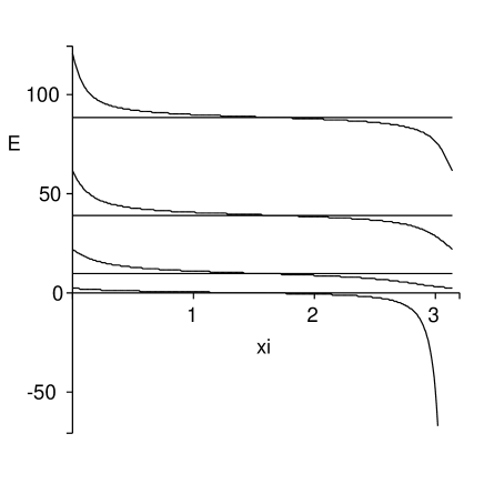
Figure 1: Lowest energy level in terms of $\xi$ for $\delta$ impurity and $\theta=1$

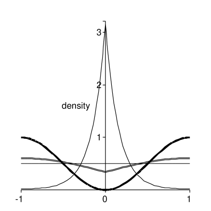
Figure 2: Density (=$|\varphi(x)|^{2}$) for various values of $\xi$.

The constant energy levels correspond to the first equation and do not depend on the impurity parameter $\xi$ as expected. The other energy levels show the effect of the impurity on the spectrum. Of special interest is the lowest energy level which exhibits a bound state for $\xi>\pi/2$. This is consistent with the fact that the coupling constant to the impurity $\eta$, given by $\eta=1/\tan\xi$, becomes negative. We have also plotted in Figure 2 the corresponding densities for different regimes. The thick curve corresponds to $\xi=0$: the impurity is completely reflecting and no transmission occurs. For $\xi=\pi/3$, the double-solid curve shows reflection and transmission for a repulsive impurity. The constant curve for $\xi=\pi/2$ is very special since for this value of $\xi$, the impurity becomes trivial in the sense that the reflection vanishes and the transmission is just $1$. This corresponds to the zero energy state. Finally, the thin curve represents the profile for $\xi=11\pi/12$: this is the bound state whose profile gets sharper and sharper as $\xi\to\pi$ (infinitely attractive impurity).

Let us move on to the case of two particles. The impurity Bethe equations read

$$\begin{cases}\exp(2ik_{1}L)\,\frac{k_{1}+k_{2}-ig}{k_{1}+k_{2}+ig}\frac{k_{1}-k_{2}-ig}{k_{1}-k_{2}+ig}=\lambda_{1}(k_{1})\\ \exp(2ik_{2}L)\,\frac{k_{2}+k_{1}-ig}{k_{2}+k_{1}+ig}\frac{k_{2}-k_{1}-ig}{k_{2}-k_{1}+ig}=\lambda_{2}(k_{2})\end{cases}$$ (4.22)

where each of the eigenvalues $\lambda_{1}(k)$, $\lambda_{2}(k)$ can be either $\pm 1$ or $\pm\frac{k\tan\xi+i}{k\tan\xi-i}$. We display on Figure 3 the corresponding lowest energy levels.

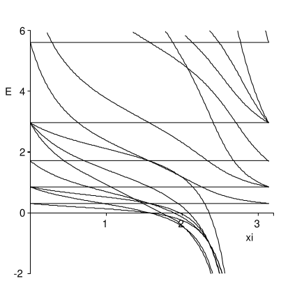
Figure 3: Lowest energy level in terms of $\xi$ for 2 particles and $\delta$ impurity

When the two eigenvalues are $\pm 1$, we obtain the constant energy levels. Otherwise, when one at least of the eigenvalues is $\pm\frac{k\tan\xi+i}{k\tan\xi-i}$, the energy levels are decreasing functions of $\xi$. Again, for special values of $\xi$ ($\xi=0$, $\xi=\pi/2$), there are degeneracies which are lifted when we tune the impurity. Finally, for $\xi>\pi/2$, the lowest energy levels give rise to bound states with the impurity (we recall that $\xi\to\pi$ corresponds to $\eta\to-\infty$ i.e. an infinitely negative coupling constant).

4.3 Asymmetric impurity in a box

In this paragraph, we give an example of an asymmetric impurity i.e. an impurity which breaks parity invariance. We simply present the one-particle case for the box boundary conditions of section 3.3. For convenience, we use the parametrization (2.9) and the impurity is characterized by a single parameter as follows

$$\alpha=1~{}~{},~{}~{}a=\sin^{2}\text{w}~{}~{},~{}~{}b=-\cos\text{w}~{}~{},~{}~{}c=\cos\text{w}~{}~{},~{}~{}d=1~{}~{},~{}~{}\text{w}\in[0,\pi)\,.$$ (4.23)

Then the Bethe equations take the form

$$e^{2ikL}=-\frac{(k^{2}-1)\cos\text{w}+ik\sqrt{4+\cos^{4}\text{w}}}{(k^{2}+1)\cos\text{w}-ik(\cos^{2}\text{w}-2)}\qquad\mbox{or}\quad e^{2ikL}=-\frac{(k^{2}-1)\cos\text{w}-ik\sqrt{4+\cos^{4}\text{w}}}{(k^{2}+1)\cos\text{w}-ik(\cos^{2}\text{w}-2)}$$ (4.24)

The two equations are never equivalent so that we do not observe level crossing (see Figure 5).

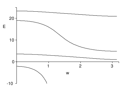
Figure 4: Lowest energy levels for a parity breaking impurity

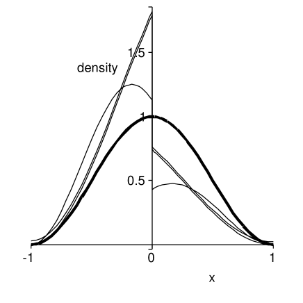
Figure 5: Density (=$|\varphi(x)|^{2}$) for the first positive energy level

On Figure 5, the density profile for the lowest positive energy level shows the striking feature of this impurity for different values of w. One can clearly see the parity invariance breaking on the thin and double-solid curves ($\text{w}=0$ and $11\pi/12$ respectively). Again for the particular value $\text{w}=\pi/2$ (the thick curve), the impurity becomes reflectionless with trivial transmission equal to $1$. Parity is restored and we observe a single excited mode in a box.

5 Conclusions and outlook

In this paper, we presented and solved the one-dimensional problem of $N$ interacting particles in the presence of an impurity. In the process of the Bethe ansatz for the wavefunction, doubling the dimension of the representation of the underlying Weyl group was a crucial ingredient with respect to previous approaches. This is reminiscent of the general RT algebras framework recently introduced and allows for an exact treatment of impurities.

We also established the impurity Bethe equations controlling the energy spectrum. Although some basic understanding emerged from the study of the simple one and two-particle cases, a systematic study of the finite size Bethe equations as well as of the integral equations arising in the thermodynamic limit is needed. This will give important non-perturbative information on the effect of the impurity on the system. This should be compared to the perturbative and effective approach of Kane and Ficher [26]. A way to tackle this problem is to compute the sound velocity $u$ and the Luttinger liquid parameter $K$ directly from our impurity Bethe equations. The result will actually give the analogs of the renormalized $u^{*}$ and $K^{*}$ in Kane and Fisher’s approach. This issue as well as other physical consequences deserve careful attention and will be investigated elsewhere.

In any case, we already observed that a tunable impurity can lift degeneracies in the energy. It can also confine asymmetrically stationary states. In this respect, we emphasize that the present approach allows for the description of unusual asymmetric impurities (and not only the standard ”delta impurity”) whose effects for finite size systems and in the thermodynamic limit will also be addressed elsewhere.

Acknowledgements: V.C. thanks the UK Engineering and Physical Sciences Research council for a Research Fellowship. N.C. is supported by the TMR Network ”EUCLID. Integrable models and applications: from strings to condensed matter”, contract number HPRN-CT-2002-00325. We acknowledge the warm support of M. Mintchev and E. Ragoucy.

References

• [1] E. H. Lieb and W. Liniger, Exact Analysis of an Interacting Bose Gas. I. The General Solution and the ground state, Phys. Rev. 130 No. 4 (1963) 1605.
• [2] M. Girardeau, Relationship between Systems of Impenetrable Bosons and Fermions in One Dimension, J. Math. Phys. 1 (1960) 516.
• [3] J. B. McGuire, Study of Exactly Soluble One-Dimensional N-Body Problems, J. Math. Phys. 5 (1964) 622.
• [4] B. Paredes et al., Tonks-Girardeau gas of ultracold atoms in an optical lattice, Nature 429 (2004) 277.
• [5] H. Bethe, Zur theorie der metalle. Eigenwerte und eingenfunktionen atomkete, Zeitschrift für Physik 71 (1931) 205.
• [6] M. Gaudin, Un système à une dimension de fermions en interaction, Phys. Lett. A24 (1967) 55.
• [7] C. N. Yang, Some exact results for the many-body problem in one dimension with repulsive delta-function interaction, Phys. Rev. Lett 19 (1967) 1312.
• [8] R. J. Baxter, Partition function of the eight-vertex lattice model, Ann. Phys. 70 (1972) 193 et J. Stat. Phys. 8 (1973) 25; Exactly solved models in statistical mechanics, (Academic Press, 1982).
• [9] M. Gaudin, Boundary Energy of a Bose Gas in One Dimension, Phys. Rev. A4 (1971) 386.
• [10] V. Caudrelier and N. Crampé, Integrable N-particle Hamiltonians with Yangian or Reflection Algebra Symmetry, J. Phys. A37 (2004) 6285 and math-ph/0310028.
• [11] B. Sutherland, Exact Results for a Quantum Many-Body Problem in One Dimension, Phys. Rev. A4 (1971) 2019.
• [12] I. V. Cherednik, Factorizing particles on a half line and root systems, Theor. Math. Phys. 61 (1984) 977.
• [13] E. K. Sklyanin, Boundary conditions for integrable quantum systems, J. Phys. A21 (1988) 2375.
• [14] E. Gutkin, Quantum Nonlinear Schrödinger Equation: Two Solutions, Phys. Rep. 167 (1988) 1.
• [15] M. Gattobigio, A. Liguori and M. Mintchev, The Nonlinear Schrödinger Equation on the Half-line, J. Math. Phys. 40 (1999) 2949 and hep-th/9811188.
• [16] A. Liguori, M. Mintchev and L. Zhao, Boundary Exchange Algebras and Scattering on the Half Line, Commun. Math. Phys. 194 (1998) 569 and hep-th/9607085.
• [17] G. Delfino, G. Mussardo and P. Simonetti, Statistical Models with a Line of Defect, Phys. Lett. B328 (1994) 123 and hep-th/9403049 ; Scattering Theory and Correlation Functions in Statistical Models with a Line of Defect, Nucl. Phys. B432 (1994) 518 and hep-th/9409076.
• [18] O.A. Castro-Alvaredo, A. Fring and F. Göhmann, On the absence of simultaneous reflection and transmission in integrable impurity systems, hep-th/0201142.
• [19] M. Mintchev, E. Ragoucy and P. Sorba, Reflection-Transmission Algebras, J.Phys. A36 (2003) 10407 and hep-th/0303187.
• [20] V. Caudrelier, M. Mintchev, É. Ragoucy and P. Sorba, Reflection transmission quantum Yang-Baxter equations, J. Phys. A38 (2005) 3431 and hep-th/0412159.
• [21] V. Caudrelier, M. Mintchev and E. Ragoucy, Solving the Quantum Nonlinear Schrödinger equation with delta-type impurity, J. Math. Phys. 46 (2004) 042703 and math-ph/0404047; The quantum non-linear Schrodinger model with point-like defect, J.Phys. A37 (2004) L367 and hep-th/0404144.
• [22] V. Caudrelier and E. Ragoucy, Spontaneous symmetry breaking in the non-linear Schrodinger hierarchy with defect, J. Phys. A38 (2005) 2241 and math-ph/0411022.
• [23] T. Cheon, T. Fulop and I. Tsutsui, Symmetry, Duality and Anholonomy of Point Interactions in One Dimension, Annals Phys. 294 (2001) 1 and quant-ph/0008123.
• [24] S. Albeverio, L. Dabrowski and P. Kurasov, Symmetries of Schrödinger Operators with Point Interactions, Lett. Math. Phys. 45 (1998) 33.
• [25] M. Hallnäs and E. Langmann, Exact solutions of two complementary 1D quantum many-body systems on the half-line, J. Math. Phys. 46 (2005) 052101 and math-ph/0404023.
• [26] C. L. Kane and M. P. L. Fisher, Transmission through barriers and resonant tunneling in an interacting one-dimensional electron gas, Phys. Rev. B46 (1992) 15233.