Many-body Landau-Zener effect at fast sweep

Abstract

The asymptotic staying probability $P$ in the Landau-Zener effect with interaction is analytically investigated at fast sweep, $\varepsilon=\pi\Delta^{2}/(2\hbar v)\ll 1$. We have rigorously calculated the value of $I_{0}$ in the expansion $P\cong 1-\varepsilon+\varepsilon^{2}/2+\varepsilon^{2}I_{0}$ for arbitrary couplings and relative resonance shifts of individual tunneling particles. The results essentially differ from those of the mean-field approximation. It is shown that strong long-range interactions such as dipole-dipole interaction (DDI) generate huge values of $I_{0}$ because flip of one particle strongly influences many others. However, in the presence of strong static disorder making resonance for individual particles shifted with respect to each other the influence of interactions is strongly reduced. In molecular magnets the main source of static disorder is the coupling to nuclear spins. Our calculations using the actual shape of the Fe₈ crystal studied in the the Landau-Zener experiments [Wernsdorfer et al, Europhys. Lett. 50, 552 (2000)] yield $I_{0}\$that is in a good agreement with the value extracted from the experimental data.

I Introduction

Landau-Zener (LZ) effect lan32 ; zen32 (see also Refs. stu32, ; akusch92, ; dobzve97, ) is a well known quantum phenomenon of transitions at avoided level crossing, see Fig. 1. LZ effect was encountered mainly in physics of atomic and molecular collisions (see, e.g., Refs. chi74, ; nak02, and references therein). In the time-dependent formulation, the LZ effect can be modeled by a two-level system (TLS)

$$\hat{H}=-\frac{1}{2}W(t)\sigma_{z}+\frac{1}{2}\Delta\sigma_{x},$$ (1)

where $\sigma_{\alpha},$ $\alpha=x,y,z$ are the Pauli matrices and

$$W(t)\equiv E_{\downarrow}(t)-E_{\uparrow}(t)$$ (2)

is the time-dependent bias of the two bare ($\Delta=0)$ energy levels. The general state of this model and the probability $P(t)$ to stay in the $\left|\downarrow\right\rangle$ state can be written as

$$\Psi(t)=a_{\downarrow}(t)\left|\downarrow\right\rangle+a_{\uparrow}(t)\left|\uparrow\right\rangle,\qquad P(t)=\left|a_{\downarrow}(t)\right|^{2}.$$ (3)

The initial condition is $W(-\infty)=-\infty$ and $P(-\infty)=1.$ If $W(t)$ changes fast, the system does not have enough time for transition to the state $\left|\uparrow\right\rangle$ and it practically remains in the state $\left|\downarrow\right\rangle,$ thus $P(t)\cong 1.$ In the opposite case of slow $W(t)$ the system mainly remains at the lower of the adiabatic energy levels

$$E_{\pm}(t)=\pm\frac{1}{2}\sqrt{W^{2}(t)+\Delta^{2}},$$ (4)

thus the asymptotic staying probability $P(\infty)\cong 0.$

The time-dependent Schrödinger equation for the Hamiltonian of Eq. (1) can be solved exactly for the linear sweep $W(t)=vt$, the result for the asymptotic staying probability being

$$P\equiv P(\infty)=e^{-\varepsilon},\qquad\varepsilon\equiv\frac{\pi\Delta^{2}}{2\hbar v}.$$ (5)

As the Schrödinger equation (SE) for a spin 1/2 is mathematically equivalent to the classical dissipationless Landau-Lifshitz equation (LLE), the effect can be viewed upon as a rotation of a classical magnetization vector. chugar02 ; gar03prb

\begin{picture}(11.0,6.0)\centerline{\hbox{\psfig{angle=-90,width=256.0748pt}}} \end{picture}

Figure 1: A pair of tunnel-splitted levels vs. energy bias $W(t)$. Here $E_{\downarrow}$ and $E_{\uparrow}$ are the bare energy levels ($\Delta=0$), whereas $E_{\pm}$ are the exact adiabatic energy levels of Eq. (4). $P$ denotes the probability to remain in the (bare) state $\left|\downarrow\right\rangle$ after crossing the resonance.

\begin{picture}(11.0,6.0)\centerline{\hbox{\psfig{angle=-90,width=256.0748pt}}} \end{picture}

Figure 2: Bare energy levels vs the sweep field $W$ for a ring of 10 two-level systems with $V_{i}=0,$ coupled by an antiferromagnetic nearest-neighbor interaction. All the lines except the two ones with the highest slopes that correspond to the states with all spins up and all spins down are strongly degenerate. The energy levels for the ferromagnetic coupling can be obtained by the upside-down transformation of this graph.

Recently the LZ effect was observed on crystals of molecular magnets Fe₈ in Refs. werses99science, ; weretal00epl, (see Refs. wer01thesis, ; sesgat03,  for a recent review). This posed a new problem of the many-body LZ effect that can be described by the Hamiltonian of the transverse Ising model

$$\hat{H}=-\frac{1}{2}\sum_{i}\left\{\left[W(t)-V_{i}\right]\sigma_{iz}+\Delta\sigma_{ix}\right\}-\frac{1}{2}\sum_{ij}J_{ij}\sigma_{iz}\sigma_{jz},$$ (6)

where $V_{i}$ are the local shifts of the resonances for individual TLSs that can be induced, for instance, by nuclear spinsweretal00prl and $J_{ij}$ is their coupling. The SE for such a system of $N\gg 1$ coupled TLSs contains $2^{N}$ time-dependent coefficients of the wave function. In the language of the time-dependent bare energy levels, there are $2^{N}$ different lines that cross each other at different values of $W,$ see Fig. 2.

Eq. (6) can be extended by taking into account coupling to environmental degrees of freedom such as phonons, as was done for one-particle LZ effect in Refs. aoram91prb, ; kaynak98prb, . One can also consider dynamics of nuclear spinssinpro03prb that are treated in a simplified way as static disorder in Eq. (6). As quantum dynamics of many-body systems far from equilibrium and coupled to environment is very involved, simplified theories using postulated rate equations (neglecting quantum-mechanical coherence) have been proposed for both the LZ effect and the relaxation out of a prepared state. prosta98prl ; cucforretadavil99epjb ; alofer01prl ; liuetal02prb ; feralo03prl All these theories consider the molecular field at the cite $i$ to determine whether the particle $i$ is in the vicinity of the resonance and thus can flip. This means that these theories are based on the mean-field approximation (MFA).

One can perform the MFA for the dissipationless system described by Eq. (6) by considering a single particle undergoing a LZ transition in the effective field being the sum of the externally sweeped field $W(t)$ and the molecular field from other particles that is determined self consistently. hamraemiysai00 This is a model of the nonlinear LZ effect that was applied to tunneling of the Bose-Einstein condensate. zobgar00 ; wuniu00 Again the problem can be reformulated in terms of a classical nonlinear LLE, see Ref. gar03prb, , although the LZ effect is a quantum-mechanical phenomenon! The MFA solution shows that ferromagnetic interactions suppress transitions since in this case the total effective field changes faster than $W(t)$ and thus the effective value of the sweep-rate parameter $\varepsilon$ in Eq. (5) becomes smaller, while antiferromagnetic interactions enhance transitions. There are, however, models with couplings of different signs for which contributions to the molecular fields cancel each other and the MFA wrongly predicts no effect of interactions.

An important special case of Eq. (6) is the so-called “spin-bag” model with the same coupling $J$ for any two spins. hamraemiysai00 ; gar03prb In the limit $N\rightarrow\infty$ with $J_{0}\equiv(N-1)J=\mathrm{const}$ the MFA for the spin-bag model becomes exact.  This model can be exactly mapped onto the model with the spin $S=N/2$ and the Hamiltonian $\widehat{H}=-W(t)S_{z}-\Delta S_{x}-2JS_{z}^{2}.$ In contrast to the model with a general interaction that is difficult to solve numerically, the spin-bag model can be numerically solved up to pretty big values of $N$ that allows to check approaching to the mean-field limit $N\rightarrow\infty$ for the original model and to the classical limit for the equivalent spin-$S$ model. gar03prb A surprising result of Ref. gar03prb, that also should be valid for a general interaction is that MFA becomes exact in the linear order in small $J,$ even without going to the limit $N\rightarrow\infty.$ Quantum corrections to the dynamics of the spin-$S$ model in the limit $S\gg 1$ (i.e., deviations from the mean-field results for the original spin-bag model) were systematically investigated in Ref. garsch04prb, .

For models with realistic finite-range interactions that are not small, the applicability of the MFA to the description of the LZ effect is not justified. In particular, one can expect large deviations from the MFA for competing interactions such as the dipole-dipole interaction (DDI). Fortunately, in the fast-sweep limit $\varepsilon\ll 1$ one can construct a rigorous perturbative expansion of the staying probability $P$ for Eq. (6) in powers of $\Delta^{2}.$ The result can be written in the formgarsch03eprint

$$P\cong 1-\varepsilon+\varepsilon^{2}/2+\varepsilon^{2}I_{0}\cong e^{-\varepsilon}+\varepsilon^{2}I_{0}$$ (7)

with $I_{0}$ depending on the coupling $J_{ij},$ resonance shifts $V_{i}$ and the sweep rate $v.$ The applicability of this expansion requires $\varepsilon I_{0}\lesssim 1.$ Eq. (7) shows whether interactions suppress transitions ($I_{0}>0$) or enhance them ($I_{0}<0$) that is not clear in the case of the DDI. On the other hand, this rigorous result can be used to test the applicability of the MFA and other approximations that can be suggested to describe the many-body LZ effect. The results of experiments measuring $P$ can be parametrized with the help of the effective splitting $\Delta^{\mathrm{eff}}$ calculated from Eq. (5):

$$\Delta^{\mathrm{eff}}=\sqrt{\frac{2\hbar v}{\pi}\ln\frac{1}{P}},$$ (8)

as was done in Ref. weretal00epl, . In the fast-sweep limit $\Delta^{\mathrm{eff}}$ should have the form following from Eq. (7):

$$\Delta^{\mathrm{eff}}=\Delta\sqrt{\frac{1}{\varepsilon}\ln\frac{1}{P}}\cong\Delta\left(1-\frac{1}{2}I_{0}\varepsilon\right).$$ (9)

Thus if $I_{0}\approx\mathrm{const},$ as is the case for strong couplings, garsch03eprint Eq. (9) allows to determine $\Delta$ and $I_{0}$ from the linear extrapolation to $\varepsilon\rightarrow 0,$ see Fig. 8 below.

The aim of this article is to explain the derivation of Eq. (7) in a more detail, provide a comparison with the MFA result, and investigate the role of the DDI in crystals of molecular magnets of non-ellipsoidal shape where the magnetostatic field is inhomogeneous and thus the resonance fields for molecules in different parts of the crystal are different. The latter is needed to make a comparison with the results of Ref. weretal00epl, on a crystal of a rectangular shape.

The remainder of this paper is organized as follows. In Sec. II we construct the perturbation scheme for the many-body LZ effect at fast sweep and derive the general expression for $I_{0}.$ In Sec. III we analyze different limiting forms of $I_{0}$ that will be used below. In this section we also consider the role of static disorder, mainly due to nuclear spins, described by $V_{i}$ in Eq. (6) and perform averaging over Gaussian distribution of $V_{i}.$ In Sec. IV we consider the influence of the DDI on the Landau-Zener transitions in samples of the ellipsoidal shape, where the dipolar field is homogeneous, as well in samples of a general shape in the case of strong static disorder. We compare our results with the experimental data of Ref. weretal00epl, in Sec. V. In Sec. VI we recollect our main results and make some proposals for future research.

II Perturbation theory for fast sweep

We consider the transverse-field Ising model, Eq. (6), with the time-linear sweep $W(t)=vt$. The wave function of the system of $N$ tunneling particles (TLSs) can be written as the expansion over the direct-product states

$$\Psi(t) = \sum_{m_{1},\ldots,m_{N}=-1,1}\mathcal{C}_{m_{1},\ldots,m_{N}}(t)\psi_{m_{1}}\otimes\ldots\otimes\psi_{m_{N}}$$

$$\psi_{-1} = \left(\begin{array}[]{c}0\\ 1\end{array}\right)=|\downarrow\rangle,\qquad\psi_{1}=\left(\begin{array}[]{c}1\\ 0\end{array}\right)=|\uparrow\rangle.$$ (14)

The initial condition for $\Psi(t)$ is $\left|\mathcal{C}_{-1,\ldots,-1}(-\infty)\right|=1$ whereas all other coefficients are zero, i.e., the system starts in the state with all spins down. One can denote this state as $\left|\downarrow\downarrow\ldots\downarrow\right\rangle.$ As the time evolves, the state of the system becomes a superposition of all possible basis states in Eq. (14). One can write the wave function in the form

$$\Psi(t) = c_{0}(t)\left|\downarrow\downarrow\ldots\downarrow\right\rangle+\sum_{i}c_{i}(t)\sigma_{i+}\left|\downarrow\downarrow\ldots\downarrow\right\rangle$$ (15)

$$+\frac{1}{2!}\sum_{ij}c_{ij}(t)\sigma_{i+}\sigma_{j+}\left|\downarrow\downarrow\ldots\downarrow\right\rangle+\ldots$$

including all possible numbers of flipped spins. Then the initial condition becomes $\left|c_{0}(-\infty)\right|=1$ and $c_{ij}(-\infty)=0,$ etc. The normalization condition for this wave function is

$$1=\left|c_{0}\right|^{2}+\sum_{i}\left|c_{i}\right|^{2}+\frac{1}{2!}\sum_{ij}\left|c_{ij}\right|^{2}+\ldots$$ (16)

The probability for a particle at the site $i$ to stay in the initial state is given by

$$P_{i} = \left|c_{0}\right|^{2}+\sum_{j\neq i}\left|c_{j}\right|^{2}+\frac{1}{2!}\sum_{j\neq i,k\neq i}\left|c_{jk}\right|^{2}+\ldots$$ (17)

$$= 1-\left|c_{i}\right|^{2}-\sum_{j}\left|c_{ij}\right|^{2}+\ldots$$

where we have used Eq. (16) to simplify the expression. The staying probability averaged over the system is

$$P=\frac{1}{N}\sum_{i}P_{i}=1-\frac{1}{N}\sum_{i}\left|c_{i}\right|^{2}-\frac{1}{N}\sum_{ij}\left|c_{ij}\right|^{2}-\ldots$$ (18)

The Schrödinger equation for the coefficients in Eq. (15) reads

$$i\hbar\dot{c}_{0} = 0\times c_{0}-\frac{\Delta}{2}\sum_{i}c_{i}$$

$$i\hbar\dot{c}_{i} = E_{i}(t)c_{i}-\frac{\Delta}{2}c_{0}-\frac{\Delta}{2}\sum_{j}c_{ij}$$

$$i\hbar\dot{c}_{ij} = E_{ij}(t)c_{ij}-\frac{\Delta}{2}\left(c_{i}+c_{j}\right)-\frac{\Delta}{2}\sum_{l}c_{ijl},$$ (19)

etc. Here $E_{i}$ and $E_{ij}$ are the eigenvalues of the Hamiltonian with $\Delta=0$ and the ground-state energy $E_{0}(t)$ subtracted

$$E_{i}(t) = -W(t)+\tilde{V}_{i},\qquad$$

$$E_{ij}(t) = -2W(t)+\tilde{V}_{i}+\tilde{V}_{j}-4J_{ij},$$ (20)

where

$$\tilde{V}_{i}\equiv V_{i}+V_{i}^{(\mathrm{int})},\qquad V_{i}^{(\mathrm{int})}\equiv 2\sum_{j}J_{ij}.$$ (21)

Whereas $V_{i}$ that enters Eq. (6) can be random, there is another contribution into resonance shifts, $V_{i}^{(\mathrm{int})},$ that can gradually change across the sample for long-range interactions such as the DDI.

For fast sweep there is little time for spin flipping and the system remains near the initial state: $\left|c_{0}(t)\right|\cong 1$ while all other coefficients are small. Since spin flipping is caused by $\Delta,$ one can consider $\Delta$ as a formal small parameter and obtain the solution of Eq. (19) in the fast-sweep limit iteratively in powers of $\Delta$. To this end, it is convenient to introduce slow amplitudes $\tilde{c}(t)$ according to

$$c_{\nu}(t)=\tilde{c}_{\nu}(t)e^{-i\Phi_{\nu}(t)},\qquad\Phi_{\nu}(t)\equiv\frac{1}{\hbar}\int_{0}^{t}dt^{\prime}E_{\nu}(t^{\prime})$$ (22)

with $\nu=i,ij$ and rewrite Eq. (19) in the form

$$\frac{d}{dt}\tilde{c}_{0} = \frac{i\Delta}{2\hbar}\sum_{i}\tilde{c}_{i}e^{-i\Phi_{i}(t)}$$

$$\frac{d}{dt}\tilde{c}_{i} = \frac{i\Delta}{2\hbar}\tilde{c}_{0}e^{i\Phi_{i}(t)}+\frac{i\Delta}{2\hbar}\sum_{j}\tilde{c}_{ij}e^{i\left[\Phi_{i}(t)-\Phi_{ij}(t)\right]}$$

$$\frac{d}{dt}\tilde{c}_{ij} = \frac{i\Delta}{2\hbar}\tilde{c}_{i}e^{i\left[-\Phi_{i}(t)+\Phi_{ij}(t)\right]}+\left(i\rightleftharpoons j\right).$$ (23)

In the last equation we have dropped the term with $\tilde{c}_{ijl}$ since we are going to calculate $P$ up to $\Delta^{4}$ and it can be shown that at this order $\tilde{c}_{ijl}$ is irrelevant. Iterating Eqs. (23) yields

$$\tilde{c}_{0} = 1+\left(\frac{i\Delta}{2\hbar}\right)^{2}\tilde{c}_{0}^{(2)}+\ldots$$

$$\tilde{c}_{i} = \frac{i\Delta}{2\hbar}\tilde{c}_{i}^{(1)}+\left(\frac{i\Delta}{2\hbar}\right)^{3}\tilde{c}_{i}^{(3)}+\ldots$$

$$\tilde{c}_{ij} = \left(\frac{i\Delta}{2\hbar}\right)^{2}\tilde{c}_{ij}^{(2)}+\ldots$$ (24)

where we have written down only relevant terms that are given by

$$\tilde{c}_{i}^{(1)}(t) = \int_{-\infty}^{t}dt^{\prime}e^{i\Phi_{i}(t^{\prime})}$$

$$\tilde{c}_{ij}^{(2)}(t) = \int_{-\infty}^{t}dt^{\prime}e^{i\left[-\Phi_{i}(t^{\prime})+\Phi_{ij}(t^{\prime})\right]}\tilde{c}_{i}^{(1)}(t^{\prime})+\left(i\rightleftharpoons j\right)$$

$$\tilde{c}_{0}^{(2)}(t) = \int_{-\infty}^{t}dt^{\prime}\sum_{i}\tilde{c}_{i}^{(1)}(t^{\prime})e^{-i\Phi_{i}(t^{\prime})}$$

$$\tilde{c}_{i}^{(3)}(t) = \int_{-\infty}^{t}dt^{\prime}e^{i\Phi_{i}(t^{\prime})}\tilde{c}_{0}^{(2)}(t^{\prime})$$ (25)

$$+\sum_{j}\int_{-\infty}^{t}dt^{\prime}\tilde{c}_{ij}^{(2)}(t^{\prime})e^{i\left[\Phi_{i}(t^{\prime})-\Phi_{ij}(t^{\prime})\right]}.$$

Now the expansion of $P_{i}$ of Eq. (17) up to $\Delta^{4}$ has the form

$$P_{i}(t) = 1-\left(\frac{\Delta}{2\hbar}\right)^{2}\left|\tilde{c}_{i}^{(1)}\right|^{2}-\left(\frac{\Delta}{2\hbar}\right)^{4}$$ (26)

$$\quad\times\left[\sum_{j}\left|\tilde{c}_{ij}^{(2)}\right|^{2}+2\mathop{\mathrm{R}e}\left(\tilde{c}_{i}^{(1)\ast}\tilde{c}_{i}^{(3)}\right)\right]+\ldots$$

It is convenient to split $P_{i}$ into the part corresponding to noninteracting particles and the part depending on the interaction, the result for the former being already known from Eq. (5), and to introduce $\varepsilon$. Thus one obtains at $t\rightarrow\infty$

$$P_{i}\cong 1-\varepsilon+\varepsilon^{2}/2+\varepsilon^{2}\sum_{j}I_{ij}\cong e^{-\varepsilon}+\varepsilon^{2}\sum_{j}I_{ij}$$ (27)

with

$$I_{ij} = \left(\frac{v}{2\pi\hbar}\right)^{2}\left[\left|\tilde{c}_{ij}^{(2)(\mathrm{ni})}(\infty)\right|^{2}-\left|\tilde{c}_{ij}^{(2)}(\infty)\right|^{2}\right]$$ (28)

$$+\left(\frac{v}{2\pi\hbar}\right)^{2}2\mathop{\mathrm{R}e}\left\{\tilde{c}_{i}^{(1)\ast}(\infty)\int_{-\infty}^{\infty}dte^{i\Phi_{i}(t)}\right.$$

$$\times\left.\left[\tilde{c}_{ij}^{(2)(\mathrm{ni})}(t)e^{-i\Phi_{ij}^{(\mathrm{ni})}(t)}-\tilde{c}_{ij}^{(2)}(t)e^{-i\Phi_{ij}(t)}\right]\right\}.$$

Here the quantities with the superscript $(\mathrm{ni})$ correspond to the noninteracting system, $J_{ij}=0.$

There is a seeming paradox in the derivation of Eqs. (27), (28). For a macroscopic system, $N\gg 1,$ even at fast sweep, $\varepsilon\ll 1,$ a macroscopic part of the particles $\varepsilon N$ is flipping out of the starting state with all spins down. However the wave function of Eq. (15) with only one or two spins flipped was used in the calculation above, whereas the coefficients $c_{ijk}$ etc. have been dropped. Our calculations is nevertheless correct, because extending of the expansion of Eq. (24) to include more terms would only lead to contributions of orders higher than $\Delta^{4}$ or, correspondingly, higher than $\varepsilon^{2}$ that we are not interested in. The seeming paradox has nothing to do with the interaction and it emerges already for a system of $N$ identical noninteracting TLSs. In this case one can just solve a one-particle problem exactly and expand $P$ of Eq. (5) up to $\varepsilon^{2}$ or, alternatively, one can solve the one-particle problem perturbatively using lines 1 and 2 of Eq. (24). The result is $P=1-\varepsilon+\varepsilon^{2}/2+\ldots.$ On the other hand, one can do the perturbative expansion for the whole system of $N$ particles up to $\varepsilon^{2}$ or higher that evidently leads to the same result. The key observation is that at any order in $\varepsilon$ (both with and without the interaction) the terms that are diverging in the limit $N\rightarrow\infty$ cancel each other, as it should be. In particular, one can see from Eqs. (27), (28) that there is no proplem in the thermodynamic limit since $I_{ij}$ decays with increasing the distance between $i$ and $j$ if the interaction $J_{ij}$ does so. In connection to the above it should be mentioned that the truncated Schrödinger equation, Eq. (23) cannot be directly solved numerically. The problem is that the solution of this equation contains all powers of $\Delta$ or $\varepsilon,$ and starting from $\Delta^{6}$ or $\varepsilon^{3}$ not all terms of the same order are taken into account. This leads to noncancellation of terms diverging in the limit $N\rightarrow\infty$ (i.e., spurious terms of order $\varepsilon^{3}N$ etc.) and thus to an unphysical behavior of the whole solution.

Calculation of the double and triple time integrals in Eq. (28) requires essential efforts. At least for the average staying propability of Eq. (18) where only the symmetrized quantity

$$I_{ij}\Longrightarrow I_{ij}^{(\mathrm{sym})}=\frac{1}{2}\left(I_{ij}+I_{ji}\right)$$ (29)

is needed and from Eq. (18) one obtains Eq. (7) with

$$I_{0}=\frac{1}{N}\sum_{ij}I_{ij}=\frac{1}{N}\sum_{ij}I_{ij}^{(\mathrm{sym})}.$$ (30)

$I_{ij}^{(\mathrm{sym})}$ can be expressed as

$$I_{ij}^{(\mathrm{sym})}=A_{ij}+\cos\left(2\pi\tilde{\delta}_{ij}\beta_{ij}\right)B_{ij}+\sin\left(2\pi\tilde{\delta}_{ij}\beta_{ij}\right)C_{ij}.$$ (31)

Here $A_{ij},$ $B_{ij},$ $C_{ij}$  are combinations of Fresnel integrals $C(x)$ and $S(x)$

$$A_{ij} = \frac{1}{2}-\frac{1}{4}\left[\frac{1}{2}-C\left(\gamma_{ij}\right)\right]^{2}-\frac{1}{4}\left[\frac{1}{2}-S\left(\gamma_{ij}\right)\right]^{2}$$ (32)

$$-\frac{1}{4}\left[\frac{1}{2}-C\left(\gamma_{ji}\right)\right]^{2}-\frac{1}{4}\left[\frac{1}{2}-S\left(\gamma_{ji}\right)\right]^{2}.$$

$$B_{ij} = -\frac{1}{2}\left[\frac{1}{2}-C\left(\gamma_{ij}\right)\right]\left[\frac{1}{2}-C\left(\gamma_{ji}\right)\right]$$ (33)

$$-\frac{1}{2}\left[\frac{1}{2}-S\left(\gamma_{ij}\right)\right]\left[\frac{1}{2}-S\left(\gamma_{ji}\right)\right].$$

$$C_{ij} = \frac{1}{2}\left[\frac{1}{2}-C\left(\gamma_{ij}\right)\right]\left[\frac{1}{2}-S\left(\gamma_{ji}\right)\right]$$ (34)

$$-\frac{1}{2}\left[\frac{1}{2}-S\left(\gamma_{ij}\right)\right]\left[\frac{1}{2}-C\left(\gamma_{ji}\right)\right],$$

and the dimensionless variable $\gamma_{ij}$ is defined by

$$\gamma_{ij} \equiv \tilde{\delta}_{ij}+\beta_{ij},\qquad\tilde{\delta}_{ij}\equiv\tilde{\alpha}_{i}-\tilde{\alpha}_{j}$$

$$\tilde{\alpha}_{i} \equiv \frac{\tilde{V}_{i}}{\sqrt{2\pi\hbar v}},\qquad\beta_{ij}\equiv\frac{4J_{ij}}{\sqrt{2\pi\hbar v}}=\frac{4J_{ij}}{\pi\Delta}\sqrt{\varepsilon}.$$ (35)

Here $\tilde{V}_{i}$ contains interaction according to its definition in Eq. (21). Note that independent arguments in Eqs. (31)–(34) are reduced interaction $\beta_{ij}$ and resonance shifts $\delta_{ij},$ thus we also will be using explicit notations of the kind

$$\Phi_{ij}\equiv\Phi(\tilde{\delta}_{ij},\beta_{ij})$$ (36)

for any of the functions $I_{ij}^{(\mathrm{sym})},$ $A_{ij},$ $B_{ij},$ and $C_{ij}.$ Similarly to Eq. (21), one can write

$$\tilde{\delta}_{ij}=\delta_{ij}+\delta_{ij}^{(\mathrm{int})}.$$ (37)

Eqs. (7) and (30)–(35) is our main result that is valid for arbitrary interactions $J_{ij}$ and resonance shifts $V_{i}$. Note that it has a pair structure and thus it can be verified against the direct numerical solution for the model of two coupled particles. Analytical form makes its application practically possible: Triple time integrals of Eq. (28) cannot be computed numerically with a reasonable precision within a reasonable time.

\begin{picture}(11.0,6.0)\centerline{\hbox{\psfig{angle=-90,width=256.0748pt}}} \end{picture}

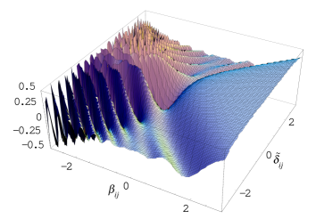
Figure 3: $I_{ij}^{(\mathrm{sym})}$ vs its independent arguments $\beta_{ij}$ and $\tilde{\delta}_{ij}.$

\begin{picture}(11.0,6.0)\centerline{\hbox{\psfig{angle=-90,width=256.0748pt}}} \end{picture}

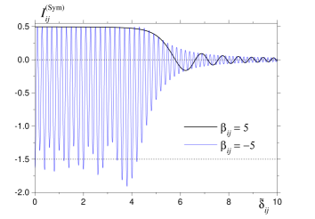
Figure 4: $I_{ij}^{(\mathrm{sym})}$ as a function of the resonance shift $\tilde{\delta}_{ij}$ for $\beta_{ij}=\pm 5.$

III Analysis of the solution

III.1 General properties and limiting cases

A three-dimensional plot of $I_{ij}^{(\mathrm{sym})}$ vs its independent arguments $\beta_{ij}$ and $\tilde{\delta}_{ij}$ is given in Fig. 3. One can see that $I_{ij}^{(\mathrm{sym})}$ has a plateau $I_{ij}^{(\mathrm{sym})}\cong 1/2$ for strong ferromagnetic interactions, $\beta_{ij}\gg 1.$ This means, according to Eqs. (7) and (30) ferromagnetic interactions suppress LZ transitions. For strong antiferromagnetic interactions, $-\beta_{ij}\gg 1,$ the value of $I_{ij}^{(\mathrm{sym})}$ oscillates between the upper bound 1/2 and the lower bound around $-3/2$(see Fig. 4), i.e., on average antiferromagnetic interactions enhance transitions. For large resonance shifts, $\left|\tilde{\delta}_{ij}\right|\gtrsim\left|\beta_{ij}\right|,$ the value of $I_{ij}^{(\mathrm{sym})}$ decays to zero. This “causality” is physically expected since two particles having resonances at very different values of the sweep field $W(t)$ do not affect LZ transitions of each other.

It can be shown that $I_{ij}^{(\mathrm{sym})}$ satisfies the sum rule

$$\int_{-\infty}^{\infty}d\delta I^{(\mathrm{sym})}(\delta,\beta)=\beta$$ (38)

that drastically simplifies the analytical results in the case of strong static disorder.

In the homogeneous case $\tilde{\delta}_{ij}=0$ one has $I_{ij}^{(\mathrm{sym})}=I_{ij}=I(0,\beta_{ij})\equiv F\left(\beta_{ij}\right),$ where

$$F\left(\beta\right)=C\left(\beta\right)\left[1-C\left(\beta\right)\right]+S\left(\beta\right)\left[1-S\left(\beta\right)\right].$$ (39)

The limiting forms of $F(\beta)$ are

$$F(\beta)\cong\left\{\begin{array}[]{ll}-\frac{3}{2}-\frac{2\sqrt{2}}{\pi\beta}\cos\left(\frac{\pi}{2}\beta^{2}+\frac{\pi}{4}\right),&-\beta\gg 1\\ \beta-\beta^{2},&|\beta|\ll 1\\ \frac{1}{2}-\frac{1}{\left(\pi\beta\right)^{2}},&\beta\gg 1.\end{array}\right.$$ (40)

For the weak interaction, $|\beta_{ij}|\ll 1,$ Eq. (7) then yields at the leading order

$$P\cong 1-\varepsilon+\frac{\varepsilon^{2}}{2}+\frac{4J_{0}}{\pi\Delta}\varepsilon^{5/2},$$ (41)

a generalization of Eq. (26) of Ref. gar03prb, for the arbitrary form of $J_{ij}.$ Note that Eq. (41) is essentially a MFA result (see a separate consideration of the MFA for our model in the Appendix) as it only depends on the zero Fourier component $J_{0}$ of the coupling $J_{ij}.$ In contrast to thermodynamic systems, here the applicability of the MFA is controlled by the strength of the interaction in addition to its radius. The correction to the mean-field result of Eq. (41) is described by the term $-\beta^{2}$ in the central line of Eq. (40). For the nearest-neighbor interaction with $z$ nearest neighbors the relative correction to the last term of Eq. (40) is $-\left[4J_{0}/(\pi\Delta)\right]\varepsilon^{1/2}/z$ that becomes small both for large $z$ and for fast sweep.

The saturation for strong ferro- and antiferromagnetic interactions in Eq. (40) corresponds to the case of well-separated resonances studied in Sec. III of Ref. gar03prb, . At fast sweep $\varepsilon\ll 1,$ LZ transitions happen in the range $W\sim W_{LZ}$ around the level crossing, wheregarsch02prb

$$W_{LZ}=\sqrt{2\pi\hbar v}=\pi\Delta/\sqrt{\varepsilon}.$$ (42)

That is, in Eq. (35) $\beta_{ij}=4J_{ij}/W_{LZ}.$ The resonances are well separated for $\left|J_{ij}\right|\gg W_{LZ},$ i.e., for $\left|\beta_{ij}\right|\gg 1.$ This limit cannot be described by the MFA. The latter becomes valid in the limit of nonseparated resonances, $\left|\beta_{ij}\right|\ll 1.$

Let us proceed to the inhomogeneous case, $\tilde{\delta}_{ij}\neq 0$. For $|\beta_{ij}|\ll 1$ Eq. (31) yields

$$I_{ij}^{(\mathrm{sym})}\cong\Xi(\tilde{\delta}_{ij})\beta_{ij}$$ (43)

with

$$\Xi(\delta) = \sin\left(\frac{\pi}{2}\delta^{2}\right)+\cos\left(\frac{\pi}{2}\delta^{2}\right)+\pi\delta\left[S\left(\delta\right)-C\left(\delta\right)\right]$$ (46)

$$\cong \left\{\begin{array}[]{cc}1-\pi\delta^{2}/2,&\delta^{2}\ll 1\\ \frac{\sqrt{2}}{\pi\delta^{2}}\cos\left(\frac{\pi}{2}\delta^{2}+\frac{\pi}{4}\right),&\delta^{2}\gg 1.\end{array}\right.$$

$\Xi(\delta)$ satisfies the sum rule

$$\int_{-\infty}^{\infty}d\delta\,\Xi(\delta)=1$$ (47)

that is a particular case of the more general Eq. (38). We will see in the Appendix that Eq. (43) also follows from the MFA.

For $\left|\tilde{\delta}_{ij}\right|-\max(|\beta_{ij}|,1)\gg 1,$ Eq. (31) yields a small value

$$I_{ij}^{(\mathrm{sym})}\cong\frac{\sqrt{2}}{\pi}\cos\left(\frac{\pi}{2}\gamma_{ji}^{2}+\frac{\pi}{4}\right)\frac{\beta_{ij}}{\tilde{\delta}_{ij}^{2}-\beta_{ij}^{2}},$$ (48)

as explained above. Note that here $\gamma_{ji}=-\tilde{\delta}_{ij}+\beta_{ij}.$ For $\left|\tilde{\delta}_{ij}\right|\gg\max(|\beta_{ij}|,1)$ this reduces to Eq. (43) with the second limiting form of Eq. (46). That is, the applicability range of Eq. (43) is larger than just $|\beta_{ij}|\ll 1.$

In the case $|\beta_{ij}|-\left|\tilde{\delta}_{ij}\right|\gg 1$ one obtains

$$I_{ij}^{(\mathrm{sym})}\cong\left\{\begin{array}[]{ll}-1/2-\cos\left(2\pi\tilde{\delta}_{ij}\beta_{ij}\right),&\beta_{ij}<0\\ 1/2,&\beta_{ij}>0.\end{array}\right.$$ (49)

For long-range interactions such as the DDI each TLS can strongly interact with many other TLSs with different strenghts $|\beta_{ij}|\gg 1,$ and the resonance shifts between different particles can be strong and different, $|\tilde{\delta}_{ij}|\gg 1.$ In this case the cosine term in Eq. (49) averages out in Eq. (30).

Neglecting the small value given by Eq. (48) and replacing the cosine term by zero in Eq. (49) one can combine the expression for $I_{ij}^{(\mathrm{sym})}$ in the case of both large arguments $\beta_{ij}$ and $\tilde{\delta}_{ij}$:

$$I_{ij}^{(\mathrm{sym})}\cong\frac{1}{2}\mathrm{sign}\left(\beta_{ij}\right)\theta\left(|\beta_{ij}|-|\tilde{\delta}_{ij}|\right).$$ (50)

Here $\theta(x)$ is the step function. Note that this form satisfies the sum rule, Eq. (38).

The terms with $\cos\left(2\pi\tilde{\delta}_{ij}\beta_{ij}\right)$ and $\sin\left(2\pi\tilde{\delta}_{ij}\beta_{ij}\right)$ in Eq. (31) represent the effect of the quantum-mechanical phase in the many-body LZ effect. The occurence of these terms is due to the possibility to come to a given final state along different ways. The latter can be seen in Fig. 2 but is absent for the usual LZ effect, Fig. 1. The quantum-mechanical amplitudes corresponding to the different ways add up with their phases in the expression for the staying probability $P$ that causes its oscillations. The minimal model that exhibits this effect is a dimer of two antiferromagnetically coupled two-level systems with shifted resonances. gar04prb Note that the effect of the quantum-mechanical phase is totally absent in the mean-field approximation.

III.2 Effect of static disorder of resonance positions

As can be seen from Eq. (21), the shifts of the resonance positions $\tilde{V}_{i}$ that enter the final formula via Eq. (35) are the sums of the two terms: The original shifts $V_{i}$ of Eq. (6) and the contribution of the interaction $J_{ij}.$ The former can arise due to different types of static disorder, including that induced by nuclear spinsweretal00prl (see below). The latter are constant and thus irrelevant ($V_{i}^{(\mathrm{int})}-V_{j}^{(\mathrm{int})}\cong 0$) within the body of the sample for short-range interactions, and in this case they only affect the particles on the surface. For long-range interactions such as the DDI, $V_{i}^{(\mathrm{int})}-V_{j}^{(\mathrm{int})}$ in general smoothly varies across the sample, depending on the sample shape.

The effect of static disorder can be accounted for by averaging Eq. (31) over stochastic values of $\alpha_{i}=\left[V_{i}/\left(\pi\Delta\right)\right]\sqrt{\varepsilon}$ with a normalized Gaussian distribution $\rho_{\alpha}(\alpha)=\left(2\pi\sigma^{2}\right)^{-1/2}\exp\left[-\alpha^{2}/\left(2\sigma^{2}\right)\right]$ and quadratic average $\left\langle\alpha_{i}^{2}\right\rangle=\sigma^{2}.$ The distribution of $\delta_{ij}=\alpha_{i}-\alpha_{j}$ is then given by the same function with $\sigma^{2}\Rightarrow 2\sigma^{2}.$ Averaging over the static disorder

$$\bar{I}^{(\mathrm{sym})}(\sigma,\delta^{(\mathrm{int})},\beta) = \int_{-\infty}^{\infty}\frac{d\delta}{\sqrt{4\pi\sigma^{2}}}\exp\left[-\frac{\delta^{2}}{4\sigma^{2}}\right]$$ (51)

$$\qquad\times I^{(\mathrm{sym})}(\delta+\delta^{(\mathrm{int})},\beta)$$

can only be done numerically in the general case. There are, however, particular cases in which it can be done analytically.

In the case of strong disorder $\sigma\gg\max(1,\left|\beta\right|)$, the integral in Eq. (51) converges at $\delta\ll\sigma,$ so that one can neglect the exponential, shift the integration variable and use Eq. (38) that yields

$$\bar{I}_{ij}^{(\mathrm{sym})}\cong\frac{1}{2\sqrt{\pi}}\frac{\beta_{ij}}{\sigma},\qquad\sigma\gg\max(1,\left|\beta_{ij}\right|).$$ (52)

Note that in this limit $\bar{I}_{ij}^{(\mathrm{sym})}$ is independent of $\delta_{ij}^{(\mathrm{int})}.$ For $\delta_{ij}^{(\mathrm{int})}=0$ and $\sigma\gg 1$ one can use the simplified form of $I_{ij}^{(\mathrm{sym})}$ given by Eq. (50) to obtain

$$\bar{I}_{ij}^{(\mathrm{sym})}\cong\frac{1}{2}\mathop{\mathrm{e}rf}\left(\frac{\beta_{ij}}{2\sigma}\right),\qquad\sigma\gg 1.$$ (53)

Indeed, for $\sigma\sim\left|\beta_{ij}\right|\gg 1$ Eq. (50) becomes correct while reducing $\left|\beta_{ij}\right|$ leads to Eq. (52).

In the case $\left|\beta\right|\ll 1$ one can use Eq. (43), where the averaged value of $\Xi$ can be found analytically for arbitrary $\sigma$ in the case $\delta^{(\mathrm{int})}=0$. One obtains

$$\bar{I}_{ij}^{(\mathrm{sym})}\cong\beta_{ij}\overline{\Xi}(\sigma),\qquad\delta^{(\mathrm{int})}=0,$$ (54)

where $\overline{\Xi}(\sigma)$ is given by

$$\overline{\Xi}(\sigma) = f\left(2\pi\sigma^{2}\right),\qquad f(x)\equiv\frac{x}{\sqrt{2(1+x^{2})}}$$ (55)

$$\times\left[\frac{x+1}{\sqrt{\sqrt{1+x^{2}}+1}}-\frac{x-1}{\sqrt{\sqrt{1+x^{2}}-1}}\right].$$

Here $f(x)$ monotonically decreases and has limiting forms

$$f(x)\cong\left\{\begin{array}[]{cc}1-x/2,&x\ll 1\\ 1/\sqrt{2x},&x\gg 1.\end{array}\right.$$ (56)

The latter limiting form,

$$\overline{\Xi}(\sigma)\cong\frac{1}{2\sqrt{\pi}\sigma},$$ (57)

follows from Eq. (47) and it is valid for $\delta^{(\mathrm{int})}\neq 0$ as well.

Let us now consider the case of weak disorder $\sigma\ll 1,$ setting $\delta^{(\mathrm{int})}=0.$ In this case the main effect arises for large negative $\beta$ [see Eq. (49)], where even small disorder can average out fast oscillations of $I_{ij}^{(\mathrm{sym})}.$ Combining Eq. (39) with Eq. (49) and using $\left\langle\cos\left(2\pi\delta\beta\right)\right\rangle=e^{-\left(2\pi\beta\sigma\right)^{2}}$ one obtains

$$\bar{I}_{ij}^{(\mathrm{sym})}\cong F(\beta_{ij})+\theta(-\beta_{ij})\left(1-e^{-\left(2\pi\beta_{ij}\sigma\right)^{2}}\right).$$ (58)

It can be seen that the limiting value $\lim_{\beta\rightarrow-\infty}F(\beta)=-3/2$ in Eq. (40) is unstable with respect to small static disorder$:$ For any $\sigma>0$ one obtains $\lim_{\beta\rightarrow-\infty}\bar{I}^{(\mathrm{sym})}(\sigma,0,\beta)=-1/2.$ The reason for that is the effect of the quantum-mechanical phase that leads to the fast oscillating terms in Eq. (31).

\begin{picture}(11.0,6.0)\centerline{\hbox{\psfig{angle=-90,width=256.0748pt}}} \end{picture}

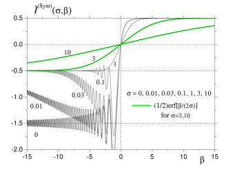
Figure 5: $\bar{I}_{ij}^{(\mathrm{sym})}$ as a function of $\beta$ for different strengths of static disorder $\sigma.$

$\bar{I}_{ij}^{(\mathrm{sym})}$ averaged over static disorder is shown as a functiion of $\beta$ for different $\sigma$ in Fig. 5. One can see that $\sigma\neq 0$ changes the asymptotic behavior of $\bar{I}_{ij}^{(\mathrm{sym})}$ at $\beta\rightarrow-\infty$ and that $\bar{I}_{ij}^{(\mathrm{sym})}$ becomes odd in $\beta$ for $\sigma\gg 1$ (in fact, already for $\sigma\gtrsim 1),$ as described by Eq. (53).

In molecular magnets distribution of resonance positions for electronic spins $V_{i}$ is mainly induced by the coupling to nuclear spins. This can be both the contact hyperfine interaction with the nuclear spins of the magnetic atoms, as in Fe₈ containing the isotope ⁵⁷Fe and in Mn₁₂, and the dipole-dipole interaction with magnetic moments of nuclear spins of non-magnetic atoms, mainly protons. The latter is small as the nuclear magneton but the number of nonmagnetic atoms interacting with the magnetic atoms is of order 10${}^{2},$ so that the total effect is quite substantial. Measurements of Ref. weretal00prl, for the resonance between the ground states $\left|\pm S\right\rangle$ ($S=10$) in Fe₈ with the standard Fe isotope (no nuclear spins on Fe atoms) yield a Gaussian line shape with the width $\sigma_{H}=0.8$ mT that is in agreement with the theoretical evaluation $\sigma_{H}=0.5$ mT. weretal00prl For the ⁵⁷Fe isotope the line width is only about two times larger, 1.2 mT and 1.1 mT, respectively. weretal00prl The dimensionless dispersion $\sigma$ introduced earlier in this section is defined similarly to Eq. (35):

$$\sigma=\frac{\sigma_{V}}{\sqrt{2\pi\hbar v}}=\frac{\sigma_{V}}{\pi\Delta}\sqrt{\varepsilon}\equiv\sigma_{0}\sqrt{\varepsilon},$$ (59)

where $\sigma_{V}=2Sg\mu_{B}\sigma_{H}$ is the dispersion in the energy units. With $\sigma_{H}=0.8$ mT one obtains $\sigma_{V}/k_{B}=21$ mK. With $\Delta/k_{B}\simeq 10^{-7}$ K for the ground-state resonance one obtains a huge value $\sigma_{0}\simeq 0.68\times 10^{5}$ that makes $\sigma$ very large even for a moderately fast sweep such as $\varepsilon\sim 10^{-2}.$ With the help of Eq. (35) one can rewrite Eq. (52) in the natural form as

$$\bar{I}_{ij}^{(\mathrm{sym})}\cong\frac{2}{\sqrt{\pi}}\frac{J_{ij}}{\sigma_{V}},\qquad\left|J_{ij}\right|\ll\sigma_{V}$$ (60)

that is independent of $\Delta.$ One can show that this result follows from the MFA as well, as all our limiting cases where $\bar{I}_{ij}^{(\mathrm{sym})}\varpropto J_{ij}$. If the disorder is so strong that $\left|J_{ij}\right|\ll\sigma_{V}$ is satisfied for all distances, including the nearest neighbors, then the many-body LZ effect can be described by the MFA.

It remains only to justify that nuclear spins can be considered as static disorder. The appropriate condition is

$$\omega_{LZ}\gg\Gamma_{\mathrm{nuc}},$$ (61)

where $\omega_{LZ}$ the characteristic frequency of the LZ transition and $\Gamma_{\mathrm{nuc}}$ is the nuclear relaxation rate. At fast sweep, $\varepsilon\ll 1,$ LZ transition occurs in the range of sweep fields defined by Eq. (42). This yields the Landau-Zener time $t_{LZ}=W_{LZ}/v=\sqrt{2\pi\hbar/v}$ and the LZ frequency

$$\omega_{LZ}=\frac{1}{t_{LZ}}=\sqrt{\frac{v}{2\pi\hbar}}=\frac{\Delta}{2\hbar}\frac{1}{\sqrt{\varepsilon}}.$$ (62)

For $\Delta/k_{B}\simeq 10^{-7}$ K one obtains $\omega_{LZ}=0.65\times 10^{4}/\sqrt{\varepsilon}$ s^-1 that grows with the sweep rate. On the other hand, recent measurements moretal04prl on Mn₁₂ yield $\Gamma_{\mathrm{nuc}}$ in the range between $10^{-1}$ and 10^-2 s^-1 for $T<1$ K. Thus nuclear spins are really slow and they can be considered as static disorder in a wide range of sweep rates. The situation is unlikely to be strongly different in Fe${}_{8}.$

IV DDI in crystals of ellipsoidal shape or with strong disorder

Let us now turn to the DDI between tunneling spins $\pm S$ of magnetic molecules aligned along the easy axis pointing in some direction $\mathbf{m},$ $\left|\mathbf{m}\right|=1$:

$$J_{ij}=E_{D}\phi_{ij},\qquad\phi_{ij}=v_{0}\frac{3\cos^{2}\theta_{ij}-1}{r_{ij}^{3}},$$ (63)

where

$$E_{D}\equiv\left(g\mu_{B}S\right)^{2}/v_{0}$$ (64)

is the dipolar energy, $v_{0}$ is the unit-cell volume, $r_{ij}$ is the distance between the sites $i$ and $j$, and $\cos\theta_{ij}=\left(\mathbf{r}_{ij}\mathbf{\cdot m}\right)/r_{ij}.$ The two mostly well known molecular magnets are Mn₁₂ and Fe${}_{8},$ both having the effective spin $S=10$. Mn₁₂ crystallizes in a tetragonal lattice with parameters $a=b=17.319$ Å, $c=12.388$ Å ($c$ is the easy axis) and $v_{0}=abc=3716$ ų. Fe₈ has a triclinic lattice with $a=10.52$ Å ($a$ is the easy axis), $b=14.05$ Å, $c=15.00$ Å, $\alpha=89.9{{}^{\circ}},$ $\beta=109.6{{}^{\circ}},$ $\gamma=109.3{{}^{\circ}}$ and $v_{0}=abc\sin\alpha\sin\beta\sin\gamma=1971$ ų (see, e.g., Ref. marchuaha01, ). Fe₈ is more convenient as a model system for us as (i) the standard Fe isotope does not have a nuclear spin that is ignored in our theory and (ii) the splitting $\Delta$ in Fe₈ has a well-defined origin and it can be estimated theoretically. One can write $\beta_{ij}$ of Eq. (35) in the form

$$\beta_{ij}=\xi\phi_{ij},\qquad\xi\equiv\xi_{0}\varepsilon^{1/2},\qquad\xi_{0}\equiv\frac{4E_{D}}{\pi\Delta}.$$ (65)

For Fe₈ $E_{D}/k_{B}=126.4$ mK and $\Delta/k_{B}\simeq 10^{-7}$ K, so that $\xi_{0}\simeq 1.6\times 10^{6}.$ Thus for not too fast sweep, $\varepsilon\sim 10^{-2},$ one has $\xi\sim 10^{5}.$ This is also an estimation for the number of spins $N_{\xi}\sim\xi$ within the distance

$$r_{c}\equiv\left(v_{0}\xi\right)^{1/3}$$ (66)

($\simeq 600$ Å for Fe${}_{8})$ that strongly interact with a given spin, $\left|\beta_{ij}\right|\gtrsim 1$.

As can be seen from Eq. (52), in the case of strong static disorder, $\sigma\gg 1$ the value of $\bar{I}_{ij}^{(\mathrm{sym})}$ is strongly reduced if $\left|\beta_{ij}\right|\lesssim\sigma.$ The corresponding characteristic length is

$$r_{\sigma}\equiv\left(v_{0}\xi/\sigma\right)^{1/3}\ll r_{c}.$$ (67)

Within this distance the interaction is still strong, $\bar{I}_{ij}^{(\mathrm{sym})}\sim 1$. The estimation for the number of spins stronly interacting with a given spin is

$$N_{\sigma}\sim\frac{r_{\sigma}^{3}}{v_{0}}=\frac{\xi}{\sigma}=\frac{4E_{D}}{\sigma_{V}}.$$ (68)

For Fe₈ one obtains $N_{\sigma}\simeq 24$ that is large but much smaller than the values of order $N_{\xi}\sim 10^{5}$ in the absence of disorder. For the superstrong disorder,

$$\sigma\gtrsim\xi\text{ \ \ \ \ \ or \ \ \ }\sigma_{V}\gtrsim E_{D},$$ (69)

there is no range where the interaction is strong, $r_{\sigma}\lesssim v_{0}^{1/3}$. For $\sigma_{V}\gg E_{D}$, as commented after Eq. (60), the mean-field description of the LZ effect with interactions becomes valid.

IV.1 Samples of ellipsoidal shape

Consider a macroscopically large specimen of ellipsoidal shape. In this case the magnetostatic field inside the homogeneously magnetized sample (the system remains in the vicinity of this state in the LZ effect at fast sweep) is homogeneous in the bulk of the sample, $\delta^{(\mathrm{int})}=0$. Thus one only has to make averaging over static disorder using Eq. (51). According to Eq. (49) $I_{ij}^{(\mathrm{sym})}$ does not diverge for $\left|\beta_{ij}\right|\rightarrow\infty.$ For $\xi\gg 1$ and $\sigma\ll\xi$ (i.e., $N_{\sigma}\gg 1$) one can replace the sum in Eq. (30) by an integral converging at $r\equiv r_{ij}\sim\min(r_{c},r_{\sigma})$ that makes the result independent of the lattice structure$:$

$$I_{0}=\int\frac{d^{3}r}{v_{0}}\bar{I}^{(\mathrm{sym})}(\sigma,\beta(\mathbf{r})),$$ (70)

where

$$\beta(\mathbf{r})=\xi\phi(\mathbf{r}),\qquad\phi(\mathbf{r})=v_{0}\frac{3\cos^{2}\theta-1}{r^{3}}.$$ (71)

To simplify the integration in Eq. (70), it is convenient to change the variables and integrate over the direction $\mathbf{r}/r$ and the value of $\beta$ instead of integrating over the direction $\mathbf{r}/r$ and the distance $r.$ At large distances where $\beta\ll 1,$ one can use Eq. (54) that makes account of the static disorder. Since $\bar{I}^{(\mathrm{sym})}(\sigma,\beta(\mathbf{r}))\varpropto\beta(\mathbf{r})$ behaves as the DDI, the result of the integration depends on the sample shape. Thus one has to be cautious with changing integration variables. One of possible ways to tackle this problem is to introduce a subtraction function, say

$$F_{\mathrm{subtr}}(\sigma,\beta(\mathbf{r}))=\frac{\beta(\mathbf{r})}{1+\beta^{2}(\mathbf{r})}\overline{\Xi}(\sigma)$$ (72)

that has a sufficiently simple form, does not diverge at small distances, $\beta\rightarrow\infty,$ and has the same behavior as $I_{ij}^{(\mathrm{\ sym})}$ at large distances, $\beta\ll 1.$ (Other types of subtraction functions differing by the cutoff at $\beta\rightarrow\infty,$ for instance, the function having $1+\left|\beta(\mathbf{r})\right|$ in the denominator, yield the same results.) With the help of Eq. (72) one can write the integral in the form

$$I_{0}=\int\frac{d^{3}r}{v_{0}}\left[\bar{I}^{(\mathrm{sym})}(\sigma,\beta(\mathbf{r}))-F_{\mathrm{subtr}}(\sigma,\beta(\mathbf{r}))\right]$$

$$\qquad\qquad+\int\frac{d^{3}r}{v_{0}}F_{\mathrm{subtr}}(\sigma,\beta(\mathbf{r})).$$ (73)

The first integral converges fast at large distances, thus it does not depend on the shape and can be rearranged by changing variables as said above. After doing that, the contribution of $F_{\mathrm{subtr}}$ into this integral disappears because of the antisymmetry $F_{\mathrm{subtr}}(-\beta,\sigma)=-F_{\mathrm{subtr}}(\beta,\sigma).$ The second integral can be calculated analytically for the actual sample shape using the results of the magnetostatics, without changing variables. The final result has the form

$$I_{0}\cong G\xi,\qquad G=G_{I}+G_{\mathrm{subtr}}.$$ (74)

Here

$$G_{I}=\frac{8\pi}{9\sqrt{3}}\mathcal{P}\int_{-\infty}^{\infty}d\beta\frac{\bar{I}^{(\mathrm{sym})}(\sigma,\beta)}{\beta^{2}}$$ (75)

where $\bar{I}^{(\mathrm{sym})}(\sigma,\beta)$ is given by Eq. (51). The subtraction contribution reads

$$G_{\mathrm{subtr}}=\left[K+\left(1/3-n^{(\mathbf{m})}\right)4\pi\right]\overline{\Xi}(\sigma),$$ (76)

where the constant $K$ is given by

$$K\equiv-\frac{8\pi}{9}\left(1-\frac{1}{\sqrt{3}}\ln\frac{\sqrt{3}+1}{\sqrt{3}-1}\right)=-0.66924,$$ (77)

and $n^{(\mathbf{m})}$ is the demagnetization coefficient depending on the sample shape and on the direction of the easy axis (i.e., the magnetization) $\mathbf{m.}$ If $\mathbf{m}$ coinsides with the $z$ axis, the symmetry axis of the ellipsoids of revolution, then $n^{(\mathbf{m})}=n^{(z)}=1/3,$ 0, and 1 for a sphere, needle and disc, respectively. In Eq. (76) the term with $K$ is the result of the actual calculation for the sphere, whereas the remainder is known from the magnetostatics.

For $\sigma\ll 1$ we use Eq. (58) to calculate $G_{I}.$ One obtains

$$G\cong-5.734+16\left(\pi/3\right)^{5/2}\sigma+\left(1/3-n^{(\mathbf{m})}\right)4\pi.$$ (78)

Here the linear-$\sigma$ contribution stems from the second term of Eq. (58) that changes the asymptotic behavior of $\bar{I}^{(\mathrm{sym})}(\sigma,\beta)$ at $\beta\rightarrow-\infty.$ The large numerical factor in front of this contribution makes $G$ very sensitive to $\sigma.$

For $\sigma\gg 1$ the integrand of in Eq. (75) is of order $1/\sigma$ and, in addition, it is nearly odd in $\beta.$ Thus the result of the integration is smaller than $1/\sigma.$ In the limit $\sigma\gg 1$ the leading term in $G$ is $G_{\mathrm{subtr}}$. From Eqs. (76) and (56) one obtains

$$G\cong\frac{K+\left(1/3-n^{(\mathbf{m})}\right)4\pi}{2\sqrt{\pi}\sigma}.$$ (79)

Using Eqs. (59), (74), and (65), one obtains

$$I_{0}\cong\frac{2}{\sqrt{\pi}}\left[K+\left(1/3-n^{(\mathbf{m})}\right)4\pi\right]\frac{E_{D}}{\sigma_{V}}$$ (80)

in the case of strong static disorder. For the ground-state resonance in Fe₈ the values of $I_{0}$ are $23.4$, $-4.44,$ $-60.0$ for the needle, sphere, and disc, respectively. $I_{0}$ changes its sign for the critical value of the demagnetizing coefficient defined by

$$n_{c}^{(\mathbf{m})}=\frac{K}{4\pi}+\frac{1}{3}=0.280.$$ (81)

One has $I_{0}>0$ for $n^{(\mathbf{m})}<n_{c}^{(\mathbf{m})}$ and $I_{0}<0$ for $n^{(\mathbf{m})}>n_{c}^{(\mathbf{m})}.$

The results of the numerical evaluation of $G$ for different values of $\sigma$ are shown in Fig. 6. Whereas $G<0$ for the sphere and disc, DDI acting predominantly antiferromagnetically and enhancing LZ transitions, the result for the needle in Eq. (74) becomes positive already for $\sigma\gtrsim 0.1$.

\begin{picture}(11.0,6.0)\centerline{\hbox{\psfig{angle=-90,width=256.0748pt}}} \end{picture}

Figure 6: $G$ of Eq. (74) for the sphere vs width of distribution of individual resonances $\sigma$. Dashed lines on the left and right are asymptotes of Eqs. (78) and (79), respectively.

IV.2 Superstrong disorder – the mean-field limit

In the MFA, $\bar{I}_{ij}^{(\mathrm{sym})}$ is given by Eq. (43) that yields Eq. (54) after averaging over static disorder. We have seen above that the MFA becomes valid for the description of the LZ effect only in the case of weak interactions $\left|J_{ij}\right|\ll\Delta/\sqrt{\varepsilon}$or in the case of superstrong disorder $\sigma_{V}\gg\max(\left|J_{ij}\right|)$ if the interaction is strong. In molecular magnets the applicability condition for the MFA is not fulfilled. Yet we consider it for the sake of completeness. For the DDI one obtains

$$I_{0}^{(\mathrm{MFA})}=\frac{1}{2\sqrt{\pi}}\frac{\xi}{\sigma}D_{\mathbf{mm}}=\frac{2}{\sqrt{\pi}}\frac{E_{D}}{\sigma_{V}}D_{\mathbf{mm}},$$ (82)

where $D_{\mathbf{mm}}\equiv$ $\mathbf{m\cdot D}_{\mathbf{m}}$

$$D_{\mathbf{mm}}\equiv\sum_{j}\phi_{ij}=D_{\mathbf{mm}}^{(\mathrm{Sphere})}+\left(1/3-n^{(\mathbf{m})}\right)4\pi$$ (83)

and $\mathbf{D}_{\mathbf{m}}$ is the dimensionless quantity proportional to the dipolar field

$$\mathbf{H}^{(D)}=\frac{g\mu_{B}S}{v_{0}}\mathbf{D}_{\mathbf{m}}$$ (84)

created on the lattice site $i$ by all other spins, $j\neq i,$ pointed in the $\mathbf{m}$ direction. One can see that $D_{\mathbf{mm}}$ replaces the universal constant $K$ in Eq. (80).

For ellipsoids of revolution with magnetization $\mathbf{m}$ directed along the symmetry axis, $D_{\mathbf{mm}}$ is independent of the lattice site $i$ in the main part of the sample, except for the vicinity of the boundaries. Note that the macroscopic field theory (magnetostatics) is insufficient to obtain Eq. (83). To this end, one can introduce a macroscopic sphere around the site $i.$ The field from the spins at sites $j$ inside this sphere can be calculated by a direct summation over the lattice and it yields the first term in Eq. (83). The field from the spins outside this sphere can be calculated macroscopically and it results into the second term in Eq. (83). For a simple cubic lattice $D_{\mathbf{mm}}^{(\mathrm{Sphere})}=0$ by symmetry and the result for $D_{zz}$ becomes purely macroscopic. For tetragonal lattices $D_{\mathbf{mm}}^{(\mathrm{Sphere})}>0$ if $a=b>c$ and $D_{\mathbf{mm}}^{(\mathrm{Sphere})}<0$ if $a=b<c.$ Direct numerical calculation yields $D_{\mathbf{mm}}^{(\mathrm{Sphere})}=5.139$ for Mn₁₂ and $4.072$ for Fe${}_{8}.$ Note that $E_{0}=-(1/2)D_{zz}E_{D}$ is the dipolar energy per site for the ferromagnetic spin alignment. Our result $E_{0}=-4.131E_{D}$ for the needle-shaped Fe₈ is in qualitative accord with $E_{0}=-4.10E_{D}$ of Ref. marchuaha01, .

One can see that unlike the rigorous value of $I_{0}$ in the limit $\xi\gg 1,$ the value of $I_{0}^{(\mathrm{MFA})}$ depends on the lattice structure via $D_{\mathbf{mm}}^{(\mathrm{Sphere})}$. For Mn₁₂ Eq. (81) with $K\Rightarrow D_{\mathbf{mm}}^{(\mathrm{Sphere})}$ yields $n_{c}^{(\mathbf{m})}=0.742$ (i.e., $I_{0}^{(\mathrm{MFA})}>0$ for $n^{(\mathbf{m})}<0.742),$ whereas for Fe₈ one obtains $n_{c}^{(\mathbf{m})}=0.657.$ In both cases it essentially differs from the prediction of our rigorous theory, Eq. (81).

IV.3 Samples of general shape with strong disorder

The strong-disorder result of Eq. (80) is valid for the samples of nonellipsoidal shape as well. Indeed, the derivation of Eq. (80) is based on the sum rule, Eq. (38), that makes the integrand in Eq. (75) linear in $\beta.$ This alone would be, however, insufficient, as the limits $\sigma\rightarrow\infty$ and $\beta\rightarrow\infty$ (i.e., $r\rightarrow 0$) are not interchangeable. Eq. (52) diverges at $r\rightarrow 0$ and it needs an appropriate regularization, whereas the true $\bar{I}_{ij}^{(\mathrm{sym})}$ does not diverge at $r\rightarrow 0.$ The regularization we have used above consists in choosing $\beta$ as the integration variable. Then approximate oddness of $\bar{I}_{ij}^{(\mathrm{sym})}$ in $\beta$ for large $\sigma$ strongly reduces the integral over $\beta$ and makes it of order $1/\sigma^{3}$ that can be neglected. This oddness is also preserved in the limit $\beta\rightarrow\infty$ for large but fixed $\sigma,$ as follows from Eq. (50). The result of the regularization at $r\rightarrow 0$ is the nontrivial constant $K$ in Eq. (80). One can see from Eq. (50) that $\bar{I}_{ij}^{(\mathrm{sym})}$ remains approximately odd in $\beta$ for large $\beta$ and $\sigma$ even in the case $\delta^{(\mathrm{int})}\neq 0$ for nonellipsoidal shapes, especially as $\delta^{(\mathrm{int})}\rightarrow 0$ for $r\rightarrow 0.$ Thus the situation in the strong-disorder case $\sigma\gg 1$ is the same for ellipsoidal and nonellipsoidal sample shapes. In both cases one switches to the integration over $\beta$ and obtains zero because the integrand is odd. Recalling that integration over $\beta$ is incompatible with taking into account the sample shape, one can correct the situation by introducing, e.g., the subtraction function of Eq. (72).

The general result thus can be written in the form

$$I_{0}=\int\frac{d^{3}r}{V}\int\frac{d^{3}r^{\prime}}{v_{0}}\frac{\overline{\Xi}(\sigma)\beta(\mathbf{r^{\prime}-r})}{1+\beta^{2}(\mathbf{r^{\prime}-r})},$$ (85)

that contains the additional averaging over the sample, $\overline{\Xi}(\sigma)$ being given by Eq. (57). For the spherical shape the result of the integration is known from Eq. (80), $I_{0}=\xi\overline{\Xi}(\sigma)K.$ The difference between the general shape and the sphere arises from the integration at large distances, where $\beta^{2}$ in the denominator of Eq. (85) can be neglected. Thus with the use of Eq. (71) one can write

$$I_{0}=\xi\overline{\Xi}(\sigma)\left[K+\int\frac{d^{3}r}{V}F(\mathbf{r})\right],$$ (86)

where the difference $F(\mathbf{r})$ is given by

$$F(\mathbf{r}) = \int_{\mathrm{Sample}}\frac{d^{3}r^{\prime}}{v_{0}}\phi(\mathbf{r^{\prime}-r})-\int_{\mathrm{Sphere}}\frac{d^{3}r^{\prime}}{v_{0}}\phi(\mathbf{r^{\prime}-r})$$ (87)

$$= \mathcal{D}_{\mathbf{mm}}(\mathbf{r})-\mathcal{D}_{\mathbf{mm}}^{(\mathrm{Sphere})}.$$

Here $\mathcal{D}_{\mathbf{mm}}(\mathbf{r})$ is the $\mathbf{m}$-component of the reduced macroscopic internal field created by the sample magnetized in the $\mathbf{m}$ direction,

$$H_{\mathbf{mm}}(\mathbf{r})=\left(g\mu_{B}S/v_{0}\right)\mathcal{D}_{\mathbf{mm}}(\mathbf{r}),$$ (88)

and $\mathcal{D}_{\mathbf{mm}}^{(\mathrm{Sphere})}=(2/3)4\pi.$ Inserting Eq. (87) into Eq. (86) yields

$$I_{0}\cong\frac{2}{\sqrt{\pi}}\left[K+\left(1/3-n^{(\mathbf{m})}\right)4\pi\right]\frac{E_{D}}{\sigma_{V}}$$ (89)

[c.f. Eq. (80)], where the average demagnetization coefficient is given by

$$\bar{n}^{(\mathbf{m})}=1-\frac{1}{4\pi}\int\frac{d^{3}r}{V}\mathcal{D}_{\mathbf{mm}}(\mathbf{r}).$$ (90)

For the needle, sphere, and disc with $\mathbf{m}$ along the symmetry axis one has $\mathcal{D}_{\mathbf{mm}}=4\pi,$ $(2/3)4\pi,$ and 0, respectively, so that Eq. (90) recovers the known results for these geometries.

\begin{picture}(11.0,6.0)\centerline{\hbox{\psfig{angle=-90,width=256.0748pt}}} \end{picture}

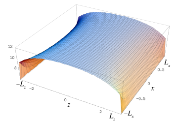
Figure 7: Dimensionless macroscopic internal field $\mathcal{D}_{\mathbf{mm}}$ of Eq. (95) in the sample of the rectangular shape with $L_{x}=L_{y}=1$ and $L_{z}=3,$ uniformly magnetized along the $z$ axis, plotted vs $x$ and $z$ for $y=0.$

For the general shape the integrals in Eq. (87) can be calculated directly with the use of

$$\phi(\mathbf{r})=\mathbf{m}\cdot v_{0}\frac{3\mathbf{n}_{\mathbf{r}}(\mathbf{m}\cdot\mathbf{n}_{\mathbf{r}})-\mathbf{e}_{z}}{r^{3}}=\mathbf{m}\cdot v_{0}\mathrm{rot}\frac{\left[\mathbf{m}\times\mathbf{n}_{\mathbf{r}}\right]}{r^{2}}$$ (91)

where $\mathbf{n}_{\mathbf{r}}\equiv\mathbf{r/}r.$ The integral formula

$$\int_{V}dV\mathrm{rot}\mathbf{F=}\int_{S}d\mathbf{S}\times\mathbf{F}$$ (92)

for an arbitrary vector function $\mathbf{F}(\mathbf{r})$ then reduces the integration to the surface. Alternatively one can use the the Bio-Savard formula

$$\mathbf{H}(\mathbf{r})=\frac{1}{c}\int d^{3}r^{\prime}\frac{\mathbf{j}\times\left(\mathbf{r-r}^{\prime}\right)}{\left|\mathbf{r-r}^{\prime}\right|^{3}}$$ (93)

with $\mathbf{j=}c\,\mathrm{rot\,}\mathbf{M}$ and $\mathbf{M=}\left(g\mu_{B}S/v_{0}\right)\mathbf{m,}$ $\left|\mathbf{m}\right|=1.$ As the molecular currents $\mathbf{j}$ are nonzero on the surface only, one obtains

$$\mathbf{H}_{\mathbf{m}}(\mathbf{r})=\frac{g\mu_{B}S}{v_{0}}\int_{S}\left[d\mathbf{S}^{\prime}\times\mathbf{m}\right]\times\frac{\mathbf{r^{\prime}-r}}{\left|\mathbf{r^{\prime}-r}\right|^{3}}.$$ (94)

For the samples of the box shape with sides $2L_{x},$ $2L_{y}$ and $2L_{z}$ with generally directed $\mathbf{m}$ the integration in Eq. (94) yields the sum of 24 arctan terms for the symmetric part of $\mathcal{D}_{\mathbf{mm}}(\mathbf{r})$ that makes the contribution into the volume average in Eq. (90)

$$\mathcal{D}_{\mathbf{mm}}^{(\mathrm{sym})}(\mathbf{r})$$ (95)

$$= (1-m_{x}^{2})\sum_{\eta_{x},\eta_{y},\eta_{z}=\pm 1}\arctan$$

$$\frac{\left(L_{x}+\eta_{x}x\right)^{-1}\left(L_{y}+\eta_{y}y\right)\left(L_{z}+\eta_{z}z\right)}{\sqrt{\left(L_{x}+\eta_{x}x\right)^{2}+\left(L_{y}+\eta_{y}y\right)^{2}+\left(L_{z}+\eta_{z}z\right)^{2}}}$$

$$+\left(xyz\Rightarrow yzx\right)+\left(yzx\Rightarrow zxy\right).$$

If $\mathbf{m}$ is directed along one of the symmetry axes of the box, the antisymmetric terms in $\mathcal{D}_{\mathbf{mm}}(\mathbf{r})$ disappear and this formula yields $\mathcal{D}_{\mathbf{mm}}(\mathbf{r}).$ The result above is illustrated in Fig. 7 for $m_{z}=1.$ Adopting Eq. (95) in Eq. (90) yields $\bar{n}^{(z)}=1/3$ for the cube and $\bar{n}^{(z)}\simeq 0.102$ for the box with proportions $L_{x}:L_{y}:L_{z}=1:5:8$ that is close to the shape of the crystal used in Ref. weretal00epl, .

V Comparison with experiment

In the sweeping experiments weretal00epl studying the $\pm S$ transitions in Fe₈ the standard LZ effect can be seen down to $dB/dt\sim 0.01$ T/s. Using $v=2Sg\mu_{B}dB/dt$ and $\varepsilon=\pi\Delta^{2}/(2\hbar v)$ with $\Delta/k_{B}\simeq 10^{-7}$ K one obtains the range $\varepsilon\lesssim 10^{-2}$ for the standard LZ effect. In the region of slower sweep $dB/dt\lesssim 0.01$ T/s (i.e., $\varepsilon\gtrsim 10^{-2}$) the effective splitting $\Delta^{\mathrm{eff}}$ calculated from Eq. (8) goes down. This suggests that here the Landau-Zener effect is strongly modified by interactions that suppress transitions. It is very instructive to replot $\exp$erimental datawerpriv as $P$ vs $\varepsilon,$ see Fig. 8a. The high plateau of $P(\varepsilon)$ at large $\varepsilon$ is similar to that for the spin-bag model with the ferromagnetic coupling and large $N,$ see, e.g., Fig. 3 of Ref. gar03prb, . One can estimate $I_{0}$ if one replots the experimental data for $\Delta^{\mathrm{eff}}$ vs $\varepsilon$ using Eq. (9), see Fig. 8. One can see that $\Delta^{\mathrm{eff}}$ is apparently linear at small $\varepsilon$. The fit ignoring the downward bump near the origin yields $I_{0}^{\exp}\simeq 11.$

\begin{picture}(11.0,6.0)\centerline{\hbox{\psfig{angle=-90,width=256.0748pt}}} \end{picture}

\begin{picture}(11.0,6.0)\centerline{\hbox{\psfig{angle=-90,width=256.0748pt}}} \end{picture}

Figure 8: Replotting experimental results of Ref. weretal00epl, vs $\varepsilon.$ (a) Staying probability $P.$  (b) $\Delta^{\mathrm{eff}}$ defined by Eq. (8). Fitting with Eq. (9) at $\varepsilon\ll 1$ yields $I_{0}\simeq 11.$

The shape of the crystal used in Ref. weretal00epl, was an elongated platelet ($l_{z}=80$ $\mu$m, $l_{y}=50$ $\mu$m, $l_{x}=10$ $\mu$m werpriv ). The crystallographic easy axis $a$ slightly deviates from the direction of the longest axis of the crystal, $l_{z}$. It is rotated by $\alpha=9{{}^{\circ}}$ in the $yz$ plane and then rotated by $\beta=7{{}^{\circ}}$ away from the $yz$ plane.werpriv Thus for this shape

$$m_{z} = \cos\alpha\cos\beta\simeq 0.9803$$

$$m_{y} = \sin\alpha\cos\beta\simeq 0.1553$$

$$m_{x} = \sin\beta\simeq 0.1219.$$ (96)

Neglecting this small tilt (i.e., setting $m_{z}=1,$ $m_{x}=m_{y}=0$) and using Eqs. (90) and (95), one obtains $\bar{n}^{(\mathbf{m})}=\bar{n}^{(z)}\simeq 0.102.$ Then Eq. (89) with $E_{D}/k_{B}=126.4$ mK and $\sigma_{V}/k_{B}=21$ mK yields $I_{0}\simeq 14.8$ that is in a good accord with $I_{0}^{\exp}\simeq 11.$ Taking into account the tilt of the easy axis improves the agreement with the experiment: $\bar{n}^{(\mathbf{m})}\simeq 0.113$ and $I_{0}\simeq 13.8.$

VI Discussion

We have analytically investigated the asymptotic staying probability $P$ in the many-body Landau-Zener effect at fast sweep, $\varepsilon\ll 1$. The coefficient $I_{0}$ in the expansion of Eq. (7) accounting for the interaction has been calculated rigorously for arbitrary interactions $J_{ij}$ and the resonance shifts $V_{i}$ in the transverse-Ising Hamiltonian of Eq. (6). We have shown that ferromagnetic interactions ($J>0)$ increase $P$ (i.e., suppress LZ transitions) whereas antiferromagnetic interactions ($J<0)$ act in the opposite direction, for the fast sweep.

The resonance shifts $\tilde{V}_{i}$ [see Eq. (21)] have been shown to reduce the value of $I_{0}$ since different particles undergoing transitions at different values of the sweep field $W$ become effectively decoupled. In all particular cases that we have considered, $I_{0}$ can be estimated as the number of neighbors that are strongly interacting with a given TLS, $\left|J_{ij}\right|\gtrsim\max(\Delta,\left|\tilde{V}_{i}-\tilde{V}_{j}\right|$) . The sign of $I_{0}$ depends on the sample shape in the case of the DDI.

Our results differ from those of the mean-field approximation. The MFA becomes valid for the description of the LZ effect only in the case of weak interactions $\left|J_{ij}\right|\ll\Delta/\sqrt{\varepsilon}$or in the case of superstrong disorder $\sigma_{V}\gg\max(\left|J_{ij}\right|)$ if the interaction is strong. Our rigorous expression for $I_{0}$ also describes models in which MFA predicts irrelevance of the interaction because of cancellation of molecular fields. Present results can be used as a “whetstone” for checking the quality of different approximations that can be suggested in the future.

For long-range interactions $J_{ij}$ that exceed $\Delta$ over large distances, huge values of $I_{0}$ are generated in the absence of the static disorder. In this case the region of fast sweeps, where a simple non-interacting LZ effect with $P\cong 1-\varepsilon$ can be observed, becomes very narrow. The biggest values of $I_{0}$ emerge in samples of ideal ellipsoidal shape, where the dipolar field is homogeneous.

For samples of general shape gradients of the dipolar field reduce the value of $I_{0}.$ The tunneling particles effectively decouple at the distances satisfying $\mathbf{r}_{ij}\cdot\nabla\mathcal{D}_{zz}\sim\phi_{ij}.$ Estimating the gradient as $\nabla\mathcal{D}_{zz}\sim L,$ where $L$ is the linear size of the specimen, one obtains the characteristic length $r_{\mathrm{inh}}\equiv\left(Lv_{0}\right)^{1/4}.$ In the strong-gradient case $r_{\mathrm{inh}}\lesssim r_{c}$ one can use Eq. (50) that yields $I_{0}\sim r_{\mathrm{inh}}^{3}/v_{0}\sim\left(V/v_{0}\right)^{1/4},$ with $V\sim L^{3}.$ This yields still large values of $I_{0}$ for macroscopic samples. $I_{0}$ even increases if the sample is elongated or flat because in this case the field becomes more uniform than in the cube. One obtains $I_{0}\sim-10^{4}$ for the crystal used in LZ experiments of Ref. weretal00epl, , if one neglects the static disorder.

Taking into account interactions with nuclear spins considered as frozen-in disorder drastically reduces $I_{0}$ for Fe₈ and yields values that agree with the values extracted from the measurements of Ref. weretal00epl, both in sign and magnitude.

It would be important to perform LZ experiments on crystals with a more flat shape for which the demagnetizing coefficient $n^{(\mathbf{m})}\gtrsim 0.28$ and Eq. (80) yields $I_{0}<0.$ In this case DDI enhances LZ transitions, and the value of $\Delta_{\mathrm{eff}}$ increases with $\varepsilon$ starting from its initial value $\Delta,$ c.f. Fig. 8. An interesting question is whether this tendency holds for larger $\varepsilon$ (slower sweep rates) as well. Our theory is applicable only for small $\varepsilon$ and it cannot answer this question. It is possible that $\Delta_{\mathrm{eff}}$ has a maximum at some $\varepsilon$ and then it falls below $\Delta,$ as indicated by our results for some simplified models of the many-body LZ effect.

Appendix A Mean-field approximation

Let us now consider the mean-field approximation for the many-body LZ effect at fast sweep and compare its results with our rigorous results obtained above. Here one has to solve the equations for single spins at different lattice sites in different effective fields:

$$i\hbar\dot{a}_{i\downarrow} = E_{i\downarrow}a_{i\downarrow}-\frac{\Delta}{2}a_{i\uparrow}$$

$$i\hbar\dot{a}_{i\uparrow} = E_{i\uparrow}a_{i\uparrow}-\frac{\Delta}{2}a_{i\downarrow},$$ (97)

where we used the definition of the wave function in the form of Eq. (3) at each lattice site $i$. Here the energies are

$$E_{i\downarrow} = \frac{1}{2}\left[H_{z}(t)-V_{i}+2\sum_{j}J_{ij}\left\langle\sigma_{j}\right\rangle\right]$$ (98)

$$= \frac{1}{2}\left[H_{z}(t)-V_{i}+2\sum_{j}J_{ij}\left(2\left|a_{i\uparrow}\right|^{2}-1\right)\right]$$

and $E_{i\uparrow}=-E_{i\downarrow}.$ Using the transformation similar to Eq. (22) one can rewrite these equations as

$$\frac{d\tilde{a}_{i\downarrow}}{dt} = \frac{i\Delta}{2\hbar}e^{i\left[\Phi_{i\downarrow}(t)-\Phi_{i\uparrow}(t)\right]}\tilde{a}_{i\uparrow}=\frac{i\Delta}{2\hbar}e^{i\Phi_{i}(t)}\tilde{a}_{i\uparrow}$$

$$\frac{d\tilde{a}_{i\uparrow}}{dt} = \frac{i\Delta}{2\hbar}e^{-i\Phi_{i}(t)}\tilde{a}_{i\downarrow}$$ (99)

with

$$\Phi_{i}(t)=\Phi_{i}^{(0)}(t)+\delta\Phi_{i}(t),$$ (100)

where

$$\Phi_{i}^{(0)}(t)=\frac{1}{\hbar}\left[\frac{vt^{2}}{2}-\tilde{V}_{i}t\right],$$ (101)

$\tilde{V}_{i}$ is defined by Eq. (21), and

$$\delta\Phi_{i}(t)=\frac{4}{\hbar}\sum_{j}J_{ij}\int_{0}^{t}dt\left|a_{j\uparrow}(t)\right|^{2}.$$ (102)

Now we can solve these equations for fast sweep $\varepsilon\ll 1$ iteratively in $\Delta$, similarly to Eq. (24) writing

$$\tilde{a}_{i\downarrow} = 1+\left(\frac{i\Delta}{2\hbar}\right)^{2}\tilde{a}_{i\downarrow}^{(2)}+\ldots$$

$$\tilde{a}_{i\uparrow} = \frac{i\Delta}{2\hbar}\tilde{a}_{i\uparrow}^{(1)}+\left(\frac{i\Delta}{2\hbar}\right)^{3}\tilde{a}_{i\uparrow}^{(3)}+\ldots$$ (103)

Further one has to expand $e^{i\Phi_{i}(t)}$ in Eq. (99) in $\left|a_{j\uparrow}(t)\right|^{2}$ that is small as $\varepsilon$ for fast sweep:

$$e^{i\Phi_{i}(t)}=e^{i\Phi_{i}^{(0)}(t)}\left[1+i\delta\Phi_{i}(t)+\ldots\right].$$ (104)

Using Eq. (35) one can show that  $\delta\Phi_{i}$ contains the product $\varepsilon\beta_{ij}.$ That is, making the expansion in powers of $\varepsilon,$ Eq. (7) within the MFA results in the expressions that are also automatically expanded in $\beta_{ij}.$ In contrast, within the rigorous formalism parameters $\varepsilon$ and $\beta_{ij}$ are split from each other and the terms of the $\varepsilon$ expansion contain general functions of $\beta_{ij}.$ Returning to the MFA, one obtains the expansion

$$\tilde{a}_{i\uparrow}^{(1)}(t) = \int_{-\infty}^{t}dt^{\prime}e^{-i\Phi_{i}^{(0)}(t^{\prime})}$$

$$\tilde{a}_{i\downarrow}^{(2)}(t) = \int_{-\infty}^{t}dt^{\prime}e^{i\Phi_{i}^{(0)}(t^{\prime})}\tilde{a}_{i\uparrow}^{(1)}(t^{\prime})$$

$$\tilde{a}_{i\uparrow}^{(3)}(t) = \int_{-\infty}^{t}dt^{\prime}e^{-i\Phi_{i}^{(0)}(t^{\prime})}\left[\tilde{a}_{i\downarrow}^{(2)}(t^{\prime})\right.$$ (105)

$$+\left.\frac{4i}{\hbar}\sum_{j}J_{ij}\int_{0}^{t^{\prime}}dt^{\prime\prime}\left|\tilde{a}_{i\uparrow}^{(1)}(t^{\prime\prime})\right|^{2}\right].$$

Now the staying probability at the site $i$

$$P_{i}(t)=1-\left|\tilde{a}_{i\uparrow}(t)\right|^{2}$$ (106)

can be expanded as

$$P_{i}(t) \cong 1-\left(\frac{\Delta}{2\hbar}\right)^{2}\left|\tilde{a}_{i\uparrow}^{(1)}(t)\right|^{2}$$ (107)

$$\quad+\left(\frac{\Delta}{2\hbar}\right)^{4}2\mathop{\mathrm{R}e}\left(\tilde{a}_{i\uparrow}^{(1)\ast}(t)\tilde{a}_{i\uparrow}^{(3)}(t)\right),$$

cf. Eq. (26). In the limit $t\rightarrow\infty,$ the terms of this formula that do not contain $J_{ij}$ just reproduce the known terms of the expansion of the LZ probability $e^{-\varepsilon}$ in powers of $\varepsilon.$ One can rewrite it in the form

$$P_{i}\cong 1-\varepsilon+\frac{\varepsilon^{2}}{2}+\varepsilon^{2}\sum_{j}I_{ij},$$ (108)

where

$$I_{ij}=\left(\frac{v}{2\pi\hbar}\right)^{2}2\mathop{\mathrm{R}e}\left(\tilde{a}_{i\uparrow}^{(1)\ast}(\infty)\tilde{b}_{ij\uparrow}^{(3)}(\infty)\right)$$ (109)

and we have defined

$$\tilde{b}_{ij\uparrow}^{(3)}(\infty)\equiv\frac{4i}{\hbar}J_{ij}\int_{-\infty}^{\infty}dte^{-i\Phi_{i}^{(0)}(t)}\int_{0}^{t}dt^{\prime}\left|\tilde{a}_{i\uparrow}^{(1)}(t^{\prime})\right|^{2}.$$ (110)

To calculate $I_{ij},$ it is convenient to introduce the dimensionless parameters $\tilde{\alpha}_{i},$ $\beta_{ij},$ and $\tilde{\delta}_{ij}$ defined by Eq. (35) and the dimensionless time variable

$$z\equiv\sqrt{\frac{v}{2\pi\hbar}}t.$$ (111)

Then Eq. (101) transforms to

$$\Phi_{i}^{(0)}(t)=\varphi_{i}(z)=\pi\left(z^{2}-2\tilde{\alpha}_{i}z\right),$$ (112)

and from Eq. (109) one obtains

$$I_{ij} = 4\pi\beta_{ij}\mathop{\mathrm{R}e}\left[f_{i}^{(1)\ast}(\infty)\int_{-\infty}^{\infty}dze^{-i\varphi_{i}(z)}\right.$$ (113)

$$\qquad\times\left.i\int_{0}^{z}dz^{\prime}\left|f_{j}^{(1)}(z^{\prime})\right|^{2}\right]$$

and

$$f_{i}^{(1)}(z)\equiv\int_{-\infty}^{z}dz^{\prime}e^{-i\varphi_{i}(z^{\prime})}.$$ (114)

One can integrate by parts in Eq. (113):

$$I_{ij} = -4\pi\beta_{ij}\mathop{\mathrm{R}e}\left[if_{i}^{(1)\ast}(\infty)\right.$$ (115)

$$\qquad\times\left.\int_{-\infty}^{\infty}dzf_{i}^{(1)}(z)\left|f_{j}^{(1)}(z)\right|^{2}\right].$$

Here $f_{i}^{(1)}(z)$ can be expressed in terms of Fresnel integrals $S(x)$ and $C(x)$:

$$f_{i}^{(1)}(z) = \int_{-\infty}^{z}dz^{\prime}e^{-i\varphi_{i}(z^{\prime})}=\int_{-\infty}^{z}dz^{\prime}e^{-i\pi\left(z^{\prime 2}-2\tilde{\alpha}_{i}z^{\prime}\right)}$$ (117)

$$= e^{i\pi\tilde{\alpha}_{i}^{2}}\int_{-\infty}^{z}dz^{\prime}e^{-i\pi\left(z^{\prime}-\tilde{\alpha}_{i}\right)^{2}}$$

$$= e^{i\pi\tilde{\alpha}_{i}^{2}}\int_{-\infty}^{z-\alpha_{i}}dz^{\prime}e^{-i\pi z^{\prime 2}}$$

$$= \frac{e^{i\pi\tilde{\alpha}_{i}^{2}}}{\sqrt{2}}\left\{\frac{1-i}{2}+C\left[\sqrt{2}(z-\tilde{\alpha}_{i})\right]\right.$$

$$\qquad-\left.iS\left[\sqrt{2}(z-\tilde{\alpha}_{i})\right]\right\}.$$

With $u=\sqrt{2}\left(z-\tilde{\alpha}_{j}\right)$ one obtains, finally

$$I_{ij} = \frac{\pi\beta_{ij}}{\sqrt{2}}\int_{-\infty}^{\infty}du\left[C(u-\sqrt{2}\tilde{\delta}_{ij})-S(u-\sqrt{2}\tilde{\delta}_{ij})\right]$$ (118)

$$\times\left[\left(\frac{1}{2}+C(u)\right)^{2}+\left(\frac{1}{2}+S(u)\right)^{2}\right].$$

For $\tilde{\delta}_{ij}=0$ this result simplifies to

$$I_{ij}=\frac{\pi\beta_{ij}}{\sqrt{2}}\int_{-\infty}^{\infty}du\left[C^{2}(u)-S^{2}(u)\right]=\beta_{ij}.$$ (119)

Moreover, it can be shown that the symmetric part of Eq. (118) defined by Eq. (29) coincides with the small-$\beta_{ij}$ expansion of the rigorous quantum mechanical result, Eqs. (30) and (43).

References

• (1) L. D. Landau, Phys. Z. Sowjetunion 2, 46 (1932).
• (2) C. Zener, Proc. R. Soc. London A 137, 696 (1932).
• (3) E.Β C.Β G. Stueckelberg, Helv. Phys. Acta 5, 369 (1932).
• (4) V. M. Akulin and W. P. Schleich, Phys. Rev. A 46, 4110 (1992).
• (5) V. V. Dobrovitski and A. K. Zvezdin, Europhys. Lett. 38, 377 (1997).
• (6) M. S. Child, Molecular Collision Theory (Academic Press, London and New York, 1974).
• (7) H. Nakamura, Nonadiabatic Transitions (World Scientific, Singapore, 2002).
• (8) E. M. Chudnovsky and D. A. Garanin, Phys. Rev. Lett. 89, 157201 (2002).
• (9) D. A. Garanin, Phys. Rev. B 68, 014414 (2003).
• (10) W. Wernsdorfer and R. Sessoli, Science 284, 133 (1999).
• (11) W. Wernsdorfer, R. Sessoli, A. Caneshi, D. Gatteschi, and A. Cornia, Europhys. Lett. 50, 552 (2000).
• (12) W. Wernsdorfer, Adv. Chem. Phys. 118, 99 (2001).
• (13) R. Sessoli and D. Gatteschi, Angew. Chem. Int. Ed. 42, 268 (2003).
• (14) W. Wernsdorfer, A. Caneshi, R. Sessoli, D. Gatteschi, A. Cornia, V. Villar, and C. Paulsen, Phys. Rev. Lett. 84, 2965 (2000).
• (15) P. Ao and J. Rammer, Phys. Rev. B 43, 5397 (1991).
• (16) Y. Kayanuma and H. Nakayama, Phys. Rev. B 57, 13099 (1998).
• (17) N. A. Sinitsyn and N. V. Prokof’ev, Phys. Rev. B 67, 134403 (2003).
• (18) N. V. Prokof’ev and P. C. E. Stamp, Phys. Rev. Lett. 80, 5794 (1998).
• (19) A. Cuccoli, A. Fort, A. Rettori, E. Adam, and J. Villain, Eur. Phys. J. B 12, 39 (1999).
• (20) J. J. Alonso and J. F. FernΓ‘ndez, Phys. Rev. Lett. 87, 097205 (2001).
• (21) J. Liu, B. Wu, L. Fu, R. B. Diener, and Q. Niu, Phys. Rev. B 65, 224401 (2002).
• (22) J. F. FernΓ‘ndez and J. J. Alonso, Phys. Rev. Lett. 91, 047202 (2003).
• (23) A. Hams, H. De Raedt, S. Miyashita, and K. Saito, Phys. Rev. B 62, 13880 (2000).
• (24) O. Zobay and B. M. Garraway, Phys. Rev. A 61, 033603 (2000).
• (25) B. Wu and Q. Niu, Phys. Rev. A 61, 023402 (2000).
• (26) D. A. Garanin and R. Schilling, Phys. Rev. B 69, 104412 (2004).
• (27) D. A. Garanin and R. Schilling, (cond-mat/0312030).
• (28) D. A. Garanin and R. Schilling, Phys. Rev. B 66, 174438 (2002).
• (29) D. A. Garanin, Phys. Rev. B 70, 212403 (2004).
• (30) A. Morello, O. N. Bakharev, H. B. Brom, R. Sessoli, and L. J. de Jongh, Phys. Rev. Lett. 93, 197202 (2004).
• (31) X. MartΓ­nes Hidalgo, E. M. Chudnovsky, and A. Aharony, Europhys. Lett. 55, 273 (2001).
• (32) W. Wernsdorfer, (private communication).