Magnetic susceptibility of a CuO2 plane in the La2CuO4 system:
I. RPA treatment of the Dzyaloshinskii-Moriya Interactions

K. V. Tabunshchyk tkir@physics.queensu.ca Department of Physics, Queen’s University, Kingston ON K7L 3N6 Canada Institute for Condensed Matter Physics, Lviv, Ukraine    R. J. Gooding Department of Physics, Queen’s University, Kingston ON K7L 3N6 Canada
Abstract

Motivated by recent experiments on undoped La2CuO4, which found pronounced temperature-dependent anisotropies in the low-field magnetic susceptibility, we have investigated a two-dimensional square lattice of S=1/2𝑆12S=1/2 spins that interact via Heisenberg exchange plus the symmetric and anti-symmetric Dzyaloshinskii-Moriya anisotropies. We describe the transition to a state with long-ranged order, and find the spin-wave excitations, with a mean-field theory, linear spin-wave analysis, and using Tyablikov’s RPA decoupling scheme. We find the different components of the susceptibility within all of these approximations, both below and above the Néel temperature, and obtain evidence of strong quantum fluctuations and spin-wave interactions in a broad temperature region near the transition.

I Introduction

Quantum magnetism of low-dimensional systems has attracted considerable attention in recent years, in part due to the strong interest in the cuprate superconductors. For example, it has been postulated that a strong antiferromagnetic (AF) exchange interaction may be responsible for the high-temperature superconductivity in these compounds.MMP

The ubiquitous structural and electronic constituent of this latter class of materials is the CuO2 plane, and in this paper we consider the magnetic properties of such planes in their undoped state. In particular, we consider the temperature dependence of the static, uniform magnetic susceptibility for a single plane in an undoped La2CuO4 crystal. This system is known to be an AF insulator with a very simple structure, namely it can be approximately thought of as one CuO2 plane stacked between LaO planes, with this structural unit repeated, in a body-centred tetragonal pattern, throughout all space. However, a small orthorhombic distortion introduces important spin-orbit couplings into the magnetic Hamiltonian, leading to an AF state with a weak canted ferromagnetic moment. These spin-orbit interactions are central to the results presented in this paper.

As was known from the start of research on the cuprate superconductors, a complete knowledge of the properties of the spin-1212\frac{1}{2} quantum Heisenberg AF on a square lattice is an absolute necessity.ManousakisRMP However, some experiments have demonstrated that a complete description of the magnetic behaviour found in, e.g. La2CuO4, requires additional physics. Examples include (i) weak ferromagnetism in the low-temperature orthorhombic (LTO) phase;Thio ; Kastner (ii) spin wave gaps with in- and out-of-plane modes;Keimer and perhaps most importantly, (iii) the unusual anisotropy of the magnetic susceptibility observed by Lavrov, Ando, Komiya and Tsukada.Ando It was this latter experiment that led us to complete a sequence of theoretical investigations on a model that should describe such a three-dimensional array of such CuO2 planes modelling La2CuO4, a structure similar to those found in many cuprate superconductors. This manuscript summarizes the first of these studies, that concerned with a single CuO2 plane, with this plane described by a near-neighbour Heisenberg model plus spin-orbit couplings as embodied by the antisymmetric and symmetric Dzyaloshinskii-Moriya (DM) interactions.Dzyaloshinskii ; Moriya

An important point needs to be raised to clarify the applicability of this work to a real physical system, such as La2CuO4. Firstly, note that according to the Mermin-Wagner theorem a two-dimensional (2D) system with a continuous symmetry cannot undergo a continuous phase transition, at any nonzero temperature, to a state with true long-ranged order. However, when one includes both the antisymmetric and symmetric DM interactions this symmetry is lifted, and thus the model that we study in this paper will have a true phase transition to an ordered phase at some nonzero temperature, which we shall label by TNsubscript𝑇𝑁T_{N}, in analogy to the Néel ordering temperature of a pure antiferromagnet. So, the ordered phase for our model of a single plane will include a weak ferromagnetic canted moment, as well as long-ranged AF order. Note that current estimatesStain of another interaction present in the physical La2CuO4 system, that being a very weak AF interlayer coupling which is usually denoted by Jsubscript𝐽perpendicular-toJ_{\perp}, is that this energy scale is close to that of the DM interactions, and thus it is likely that both this exchange and the DM interactions are roughly equally responsible for the observed transition. This serves to emphasize that our study of a single plane is not expected to accurately explain all of the observed magnetic properties of La2CuO4; in fact, this work stands alone as a theoretical study of an isolated plane, but it is of considerable interest to learn which experimental data can and which data can not be explained by such a single-plane model.

We focus on the role of the DM interaction between the neighbouring spins in a CuO2 plane. This interaction arises from the orthorhombic distortion in La2CuO4 (which is associated with the small tilt of the CuO6 octahedra) together with the spin-orbit interaction. The DM interaction leads to a small canting of the Cu spins out of the plane, so that the weak ferromagnetic order appears in each CuO2 plane, and subsequently allows for the formation of 3D AF order. This allows one to observe a pronounced peak in zero-field magnetic susceptibility,notation χc(T)superscript𝜒𝑐𝑇\chi^{c}(T), and the earliest work on the importance of this interaction focused on DM physics. To be specific, Thio et al.Thio ; Thio1 analyzed their susceptibility data using a Landau theory expanded to sixth order, for a 2D Heisenberg antiferromagnet with interlayer coupling and the DM-generated terms. They obtained reasonable fits of their theory to the susceptibility and field dependent magnetization data, and deduced parameters which characterized magnetic properties of the La2CuO4 system. As we shall explain below, we believe that the necessity of incorporating such higher-order terms into their fits is suggestive of the important role played by spin-wave interactions, a conclusion consistent with the results presented in this, and our future manuscripts on this problem.

Investigations of the magnetic ground state of La2CuO4 were performed by several groups of authors, usually within the framework of the linear spin-wave (SW) theory. The calculations were based on an effective model Hamiltonian derived by Moriya’s perturbation theoryMoriya applied to Hubbard type Hamiltonians by taking into account the spin-orbit coupling. In the most general form, the effective spin Hamiltonian, in addition to the isotropic exchange interaction, includes the above-mentioned antisymmetric and symmetric DM interactions. The first microscopic derivation of the spin Hamiltonian was performed by Coffey, Rice, and Zhang;Coffey2 they estimated the antisymmetric DM coupling constants and showed that when the DM vectors alternate a net ferromagnetic moment may be generated in the ground state. Shekhtman, Entin-Wohlman, and AharonyAharony1 subsequently showed that the symmetric anisotropies contribute to the magnetic energy in the same order as the antisymmetric DM anisotropy, and can never be neglected. Several groupsKoshibae ; Aharony2 ; Stain reexamined the Moriya’ s theory and found expressions for the effective spin Hamiltonian which includes both types of anisotropies. The linear SW theory applied to such models at T=0𝑇0T=0 allows one to obtain previously reported values of the spin-wave gaps at the centre of the 2D Brillouin zone, as well as to estimate the magnitudes of the anisotropic-exchange interactions. However, a detailed consideration of the model with the antisymmetric and symmetric DM anisotropies at nonzero temperatures is up to now absent from the literature.

A very rough and simple approximation which can be used to study the effective magnetic model at finite temperatures is the mean field approximation (MFA). The MFA ignores effects of fluctuations and correlations between the spins, hence, it fails for T𝑇T near TNsubscript𝑇𝑁T_{N} and gives no short-range order above the transition temperature. At very low T𝑇T the noninteracting SW theory is useful, and it gives a successful prediction of the energy of low-lying excited states, and correctly reproduces the dominant term in the low-T𝑇T magnetization. But, it fails near the phase transition point. To analyze the high temperature behaviour the 1/T1𝑇1/T expansion method can be employed. But, since the La2CuO4 crystal ordering temperature is much smaller than the magnitude of the superexchange interaction (TN<<Jmuch-less-thansubscript𝑇N𝐽T_{\rm N}<<J), the high-temperature expansion (to the first few orders in J/T𝐽𝑇J/T) is not able to discuss the temperature region of interest, that is T𝑇T near the transition temperature.

In the present paper time we consider the 2D spin-1212\frac{1}{2} anisotropic quantum Heisenberg antiferromagnet over the entire temperature range including both the symmetric and anti-symmetric DM interactions. We employ the technique of double-time temperature-dependent Green’s functions within the framework of the random-phase approximation (RPA). The first time such a scheme was used was by Tyablikov,Tyablikov and he applied this formalism to the Heisenberg ferromagnet (the RPA for magnetic models is often referred to as Tyablikov’s decoupling approximation). This work was generalized by LiuLiu to obtain the longitudinal correlation function, and this latter study is important in the development presented in our paper. The important feature of this technique is that it deals with the entire temperature region and is in a good agreement with the SW theory at low-T𝑇T, as well as with 1/T1𝑇1/T expansions at high-T𝑇T. In this paper, within such a scheme, we find the transition temperature at which long-range order would be established for an isolated plane. We obtain the excitation spectrum, sublattice magnetization and susceptibility tensor as function of temperature and coupling constants. We also employ the MFA and SW theories to compare results of all of these approximation schemes, and note the essential differences between them.

Of course, many investigations of the 2D spin-1212\frac{1}{2} have been completed previous to this work. We have already mentioned the most popular and simple methods to study spin models, that is phenomenological Landau theory, linear SW theory, the MFA, and high-temperature expansions. They yield an analytical description of a wide range of physical properties and are very useful for practical purposes. At the same time the great progress in the understanding of the ground state, thermodynamic properties, and spin dynamics of the Heisenberg magnets was made with the use of the newer and more complicated analytical schemes. Arovas and AuerbachArovas used a path-integral formulation of the MFA theory within the Schwinger-boson representation. This method corresponds to the large-N𝑁N limit of the generalized SU(N)𝑁(N) model; however, various difficulties with this method have been discussed in the literature.sarker89 ; desilva02 TakahashiTakahashi has formulated and successfully applied the so-called modified SW theory to the Heisenberg model which reproduced the results of conventional SW theory and is closely related to the Schwinger-boson theory. For the one dimensional chain, Takahashi’s modified SW theory yields very good agreement with Bethe ansatz results, as well as for the 2D classical ferromagnet at low-T𝑇T (in that it agrees with Monte Carlo results). A self-consistent SW theory that is based on the boson-pseudofermion representation, was developed to study thermodynamics of 2D systems, and was also applied to S1𝑆1S\geq 1 systems with an Ising-anisotropy 2D magnets.Irkhin An important feature of all these methods is that they can be used to describe both the ordered and disordered (i.e. the case of no long-range order) states.

Other related work includes: (i) The fermion representation to perform a 1/N1𝑁1/N expansion was used by Affleck and Marston,Affleck large-S𝑆S 2D Heisenberg antiferromagnet in the long-wavelength limit; and (ii) based on the diagrammatic method for the spin operators, the thermodynamics and the longitudinal spin dynamics of Heisenberg magnets were studied.Sherman ; Izyumov However, the most note-worthy success in the investigation of this system is the work i of Chakravarty et al.Chakravarty , who used a renormalization-group approach to the quantum non-linear σ𝜎\sigma model, the latter of which describes the low-T𝑇T behaviour of the 2d Heisenberg AF in the long-wavelength limit.

As will become apparent below, the formalism that we have chosen to implement is more appropriate for this problem than any of those listed above, or the theories listed above are too complicated to invoke when one goes beyond the 2D spin-1212\frac{1}{2} Heisenberg AF and includes spin-orbit couplings.

The above few paragraphs summarize theoretical efforts that were directed towards the understanding of the 2D S=1/2 square lattice AF. The application of these and related work to describe the magnetic properties of so-called single-layer cuprate superconductors, such as La2CuO4, has attracted the attention of many theorists, and fortunately an extensive review of this work, written by Johnston, already exists.johnston In this reviewjohnston one can find the comparison of the temperature dependence of the magnetic susceptibility for an AF Heisenberg square lattice calculated by different analytical methods and quantum Monte Carlo calculations, and, apart from the (post-review) data given by Lavrov et. al.Ando , the application of the analytical predictions together with the numerical results show very good fitting to the experimental data for the different single-layer cuprate compounds.

Our paper is organized as follows. In §II we present the model Hamiltonian that we will study, introduce a convenient coordinate transformation with which it is simple to complete analytical calculations, and then derive the transformation that relates the static uniform susceptibility in both coordinate systems. In §III we derive and describe the MFA results, and then in §IV we present our derivations from applying the Tyablikov/Liu approach to our model Hamiltonian. In §V we present a detailed examination of numerical results that follow from our work, including a comparison of MFA, RPA and SW theories. Finally, in §VI we summarize our paper including a brief discussion of the remainder of the work that we have completed on the full three-dimensional problem.

II Model and Definitions:

II.1 Model Hamiltonian and the initial representation

We consider a model for the Cu spins that are present in the CuO2 planes of a La2CuO4 crystal in the low-temperature orthorhombic (LTO) phase and employ a square lattice with nearest-neighbour interactions described by the following effective magnetic Hamiltonian:Koshibae ; Aharony1

H=Ji,j𝐒i𝐒j+i,j𝐃ij(𝐒i×𝐒j)+i,j𝐒iΓij𝐒j.𝐻𝐽subscript𝑖𝑗subscript𝐒𝑖subscript𝐒𝑗subscript𝑖𝑗subscript𝐃𝑖𝑗subscript𝐒𝑖subscript𝐒𝑗subscript𝑖𝑗subscript𝐒𝑖subscriptΓ𝑖𝑗subscript𝐒𝑗H=J\sum_{\langle i,j\rangle}{\bf S}_{i}\cdot{\bf S}_{j}+\sum_{\langle i,j\rangle}{\bf D}_{ij}\cdot({\bf S}_{i}\times{\bf S}_{j})+\sum_{\langle i,j\rangle}{\bf S}_{i}\cdot\overleftrightarrow{\Gamma}_{ij}\cdot{\bf S}_{j}. (1)

This Hamiltonian consists of the superexchange interaction together with the antisymmetric Dzyaloshinskii-Moriya (DM) interaction (𝐃𝐃\bf D term) and the symmetric pseudodipolar interaction (ΓΓ\overleftrightarrow{\Gamma} term). As was discussed in the introduction, the DM and pseudodipolar anisotropies arise as a result of the mixture of Hubbard-type interaction energies and spin-orbit coupling in the low symmetry crystal structure.

For the LTO phase, we use anisotropic interactions given by of the following form

𝐃ab=d2(1,1,0),𝐃ac=d2(1,1,0),formulae-sequencesubscript𝐃𝑎𝑏𝑑2110subscript𝐃𝑎𝑐𝑑2110\displaystyle{\bf D}_{ab}=\frac{d}{\sqrt{2}}(-1,1,0),\;\;{\bf D}_{ac}=\frac{d}{\sqrt{2}}(-1,-1,0), (2)

and

Γab=(Γ1Γ20Γ2Γ1000Γ3),Γac=(Γ1Γ20Γ2Γ1000Γ3),formulae-sequencesubscriptΓ𝑎𝑏subscriptΓ1subscriptΓ20subscriptΓ2subscriptΓ1000subscriptΓ3subscriptΓ𝑎𝑐subscriptΓ1subscriptΓ20subscriptΓ2subscriptΓ1000subscriptΓ3\displaystyle\overleftrightarrow{\Gamma}_{ab}{=}\left(\begin{array}[]{ccc}\Gamma_{1}&\Gamma_{2}&0\\ \Gamma_{2}&\Gamma_{1}&0\\ 0&0&\Gamma_{3}\end{array}\right)\!\!,\;\overleftrightarrow{\Gamma}_{ac}{=}\left(\begin{array}[]{ccc}\Gamma_{1}&-\Gamma_{2}&0\\ -\Gamma_{2}&\Gamma_{1}&0\\ 0&0&\Gamma_{3}\end{array}\right)\!\!, (9)

where the corresponding coordinates, in what we refer to as the “initial representation” in the LTO phase, are shown in Fig. 1(a). Note that the DM vector given in Eq. (2) alternates in sign on successive bonds in the ab𝑎𝑏a-b and in the ac𝑎𝑐a-c direction of the lattice, as is represented schematically by the double arrows in Fig. 1(b).

Refer to caption

(a)                                         (b)

Figure 1: (a) Coordinates in the initial representation. (b) Thin arrows — the Cu spins, open arrows — the DM vectors.

We mention that the symmetric tensor ΓΓ\overleftrightarrow{\Gamma} has been obtained by several authorsAharony1 ; Bonesteel ; Koshibae ; Aharony2 ; Stain in different forms. We have chosen the general form of this tensor, from which other specialized choices can be extracted. For instance, the form of the symmetric tensor obtained by Koshibae, Ohta, and MaekawaKoshibae can be recovered from this definition if Γ3=Γ2Γ1subscriptΓ3subscriptΓ2subscriptΓ1\Gamma_{3}=\Gamma_{2}-\Gamma_{1}.

In the LTO phase the classical ground state is determined uniquely,Koshibae ; Aharony2 and below the Néel temperature the Cu spin structure shows long-range antiferromagnetic order with weak ferromagnetism (viz. all spins cant out of the plane). To be concrete, in the classical ground state the spins are canted from in-plane antiferromagnetic order by a small angle given by

θ=12tan1(d/2J+12(Γ1+Γ3)),𝜃12superscript1𝑑2𝐽12subscriptΓ1subscriptΓ3\theta=\frac{1}{2}\tan^{-1}\Big{(}\frac{d/\sqrt{2}}{J+\frac{1}{2}(\Gamma_{1}+\Gamma_{3})}\Big{)}, (10)

and each plane has a net ferromagnetic moment in the z𝑧z direction perpendicular to the CuO2 planes (weak ferromagnetism).

In the simplified case of the zero pseudodipolar interaction (Γ=0Γ0\overleftrightarrow{\Gamma}=0) it was foundCoffey1 ; Coffey2 that the ground-state spin configuration exhibits the rotational symmetry about the DM vector which is the origin of the Goldstone mode in the spin-wave spectrum. Since in this simplified case there is a continuous symmetry in the ground state, the thermal fluctuations destroy the long-range order for any T>0𝑇0T>0, according to the Mermin and Wagner theorem.merminwagner In the general case of the model Hamiltonian of Eq. (1), the continuous symmetry no longer exists and the spin-wave spectrum is gapped in the long wavelength limit 𝒒=0𝒒0\boldsymbol{q}=0. Consequently, the effect of fluctuations is reduced. That is, the DM (𝐃0𝐃0{\bf D}\neq 0) together with pseudodipolar (Γ0Γ0\overleftrightarrow{\Gamma}\neq 0) interactions can give rise to long-range order for low (but nonzero) temperatures even for the purely two-dimensional case (T>N0{}_{\rm N}>0), and the Mermin and Wagner theorem does not preclude the possibility of a nonzero sublattice magnetization for nonzero temperatures in this general case. (Note that his does not imply that the transition to 3d long-ranged magnetic order is not influenced by the inter-planar exchange coupling, but simply that this latter coupling is not, in general, necessary to achieve such order.)

II.2 Characteristic representation

In solving this system, it is more convenient (theoretically) to transform from the initial representation, given above, to the characteristic representation (CR) in which the quantization axis (z𝑧z) is in the direction of a classical moment characterizing the ground state. In the present case there are two such classical vectors in the direction of the canted moments (recall that we are considering only a single CuO2 plane). Therefore, we introduce two rotated coordinate systems, as shown in Fig. 2. Spin degrees of freedom in the initial representation are denoted by {Si}subscript𝑆𝑖\{S_{i}\}, but in the characteristic representation we use {σi}subscript𝜎𝑖\{\sigma_{i}\}. (We follow the notation that i𝑖i-sites belong to sublattice 1, whereas j𝑗j-sites belong to sublattice 2.) For the sites of sublattice 1 we apply a transformation of the form

(σixσiyσiz)superscriptsubscript𝜎𝑖𝑥superscriptsubscript𝜎𝑖𝑦superscriptsubscript𝜎𝑖𝑧\displaystyle\left(\begin{array}[]{c}\sigma_{i}^{x}\\ \sigma_{i}^{y}\\ \sigma_{i}^{z}\\ \end{array}\right) =\displaystyle= 12(sinθ+1sinθ12cosθsinθ1sinθ+12cosθ2cosθ2cosθ2sinθ)(1212012120001)(SixSiySiz)12𝜃1𝜃12𝜃𝜃1𝜃12𝜃2𝜃2𝜃2𝜃1212012120001superscriptsubscript𝑆𝑖𝑥superscriptsubscript𝑆𝑖𝑦superscriptsubscript𝑆𝑖𝑧\displaystyle\frac{1}{2}\left(\begin{array}[]{ccc}\sin\theta{+}1&\sin\theta{-}1&{-}\sqrt{2}\cos\theta\\ \sin\theta{-}1&\sin\theta{+}1&{-}\sqrt{2}\cos\theta\\ \sqrt{2}\cos\theta&\sqrt{2}\cos\theta&2\sin\theta\\ \end{array}\right)\left(\begin{array}[]{ccc}\frac{1}{\sqrt{2}}&\frac{1}{\sqrt{2}}&0\\ \frac{-1}{\sqrt{2}}&\frac{1}{\sqrt{2}}&0\\ 0&0&1\\ \end{array}\right)\left(\begin{array}[]{c}S_{i}^{x}\\ S_{i}^{y}\\ S_{i}^{z}\\ \end{array}\right) (23)
=\displaystyle= 12(1sinθcosθ1sinθcosθ02cosθ2sinθ)(SixSiySiz),121𝜃𝜃1𝜃𝜃02𝜃2𝜃superscriptsubscript𝑆𝑖𝑥superscriptsubscript𝑆𝑖𝑦superscriptsubscript𝑆𝑖𝑧\displaystyle\frac{1}{\sqrt{2}}\left(\begin{array}[]{ccc}1&\sin\theta&-\cos\theta\\ -1&\sin\theta&-\cos\theta\\ 0&\sqrt{2}\cos\theta&\sqrt{2}\sin\theta\\ \end{array}\right)\left(\begin{array}[]{c}S_{i}^{x}\\ S_{i}^{y}\\ S_{i}^{z}\\ \end{array}\right)\!\!, (30)

and for sublattice 2

(σjxσjyσjz)=12(1sinθcosθ1sinθcosθ02cosθ2sinθ)(SjxSjySjz).superscriptsubscript𝜎𝑗𝑥superscriptsubscript𝜎𝑗𝑦superscriptsubscript𝜎𝑗𝑧121𝜃𝜃1𝜃𝜃02𝜃2𝜃superscriptsubscript𝑆𝑗𝑥superscriptsubscript𝑆𝑗𝑦superscriptsubscript𝑆𝑗𝑧\displaystyle\left(\begin{array}[]{c}\sigma_{j}^{x}\\ \sigma_{j}^{y}\\ \sigma_{j}^{z}\\ \end{array}\right)=\frac{1}{\sqrt{2}}\left(\begin{array}[]{ccc}1&\sin\theta&\cos\theta\\ -1&\sin\theta&\cos\theta\\ 0&-\sqrt{2}\cos\theta&\sqrt{2}\sin\theta\\ \end{array}\right)\!\!\!\left(\begin{array}[]{c}S_{j}^{x}\\ S_{j}^{y}\\ S_{j}^{z}\\ \end{array}\right)\!\!. (40)

The quantization axes (z𝑧z) of the new spin operators σisubscript𝜎𝑖\sigma_{i} and σjsubscript𝜎𝑗\sigma_{j} coincide with the unit vectors in the direction of canted moments moments Fig. 2.

Refer to caption
Figure 2: Numbered arrows represent the Cu spin structure in a CuO2 plane. Two sublattices 1 and 2 are introduced. For each sublattice the spin coordinate system within the characteristic representation (i.e. after the transformations given by (30) and (40)) is shown. The thin net is shown only to simplify the visualization of the spin structure.

The model Hamiltonian of Eq. (1) in terms of the new operators σ𝜎\sigma reads

HCR=i,jab{A(σi+σj+σiσj+)\displaystyle H_{\rm CR}=\sum_{\langle i,j\rangle_{ab}}\left\{A(\sigma^{+}_{i}\sigma^{-}_{j}+\sigma^{-}_{i}\sigma^{+}_{j})\right. Bσi+σj+superscript𝐵subscriptsuperscript𝜎𝑖subscriptsuperscript𝜎𝑗\displaystyle\!\!\!\!\!\!-B^{*}\sigma^{+}_{i}\sigma^{+}_{j}
BσiσjJ2σizσjz}\displaystyle\!\!\!\!\!\!\left.-B\sigma^{-}_{i}\sigma^{-}_{j}-J_{2}\sigma^{z}_{i}\sigma^{z}_{j}\right\}
+i,jac{A(σi+σj+σiσj+)+Bσi+σj+\displaystyle+\sum_{\langle i,j\rangle_{ac}}\left\{A(\sigma^{+}_{i}\sigma^{-}_{j}+\sigma^{-}_{i}\sigma^{+}_{j})\right.+B\sigma^{+}_{i}\sigma^{+}_{j}
+BσiσjJ2σizσjz},\displaystyle\!\!\!\!\!\!\left.+B^{*}\sigma^{-}_{i}\sigma^{-}_{j}-J_{2}\sigma^{z}_{i}\sigma^{z}_{j}\right\},

where we introduced the following definitions

J1=J+Γ1,subscript𝐽1𝐽subscriptΓ1\displaystyle J_{1}=J+\Gamma_{1},
J2=12(Γ1Γ3)+(d2/2)+[J+12(Γ1+Γ3)]2,subscript𝐽212subscriptΓ1subscriptΓ3superscript𝑑22superscriptdelimited-[]𝐽12subscriptΓ1subscriptΓ32\displaystyle J_{2}=\frac{1}{2}(\Gamma_{1}-\Gamma_{3})+\sqrt{(d^{2}/2)+[J+\frac{1}{2}(\Gamma_{1}+\Gamma_{3})]^{2}},
J3=12(Γ1Γ3)+(d2/2)+[J+12(Γ1+Γ3)]2,subscript𝐽312subscriptΓ1subscriptΓ3superscript𝑑22superscriptdelimited-[]𝐽12subscriptΓ1subscriptΓ32\displaystyle J_{3}=-\frac{1}{2}(\Gamma_{1}-\Gamma_{3})+\sqrt{(d^{2}/2)+[J+\frac{1}{2}(\Gamma_{1}+\Gamma_{3})]^{2}},
J4=Γ2sinθ+d2cosθ,subscript𝐽4subscriptΓ2𝜃𝑑2𝜃\displaystyle J_{4}=-\Gamma_{2}\sin\theta+\frac{d}{\sqrt{2}}\cos\theta,
(42)
A=J1J34,B=J42+iJ1+J34.formulae-sequence𝐴subscript𝐽1subscript𝐽34𝐵subscript𝐽42isubscript𝐽1subscript𝐽34\displaystyle A=\frac{J_{1}-J_{3}}{4},\qquad B=\frac{J_{4}}{2}+{\rm i}\frac{J_{1}+J_{3}}{4}. (43)

The subscripts i,jabsubscript𝑖𝑗𝑎𝑏\langle i,j\rangle_{ab} and i,jacsubscript𝑖𝑗𝑎𝑐\langle i,j\rangle_{ac} in the summations of Eq. (LABEL:eq:H_CR) imply the nearest neighbours in the ab𝑎𝑏ab and ac𝑎𝑐ac directions, as shown in Fig. 1(b).

The form of the Hamiltonian in the characteristic representation is similar to an XYZ model, but is clearly more complicated since terms of the form σiσjσi+σj+superscriptsubscript𝜎𝑖superscriptsubscript𝜎𝑗superscriptsubscript𝜎𝑖superscriptsubscript𝜎𝑗\sigma_{i}^{-}\sigma_{j}^{-}-\sigma_{i}^{+}\sigma_{j}^{+} are present, which thus imply terms like SixSjysubscriptsuperscript𝑆𝑥𝑖subscriptsuperscript𝑆𝑦𝑗S^{x}_{i}S^{y}_{j}. Thus, we can extract from our results, in this representation, the magnetic susceptibility of the XYZ calculated in both the mean-field and random phase approximations, by setting the imaginary part B=0𝐵0B=0. We will consider numerical results for this simpler model in a future publication.

II.3 Magnetic susceptibility in the initial and characteristic representations

We consider the response of the system, described by the Hamiltonian H𝐻H in either the initial (Eq. (1)) or characteristic representation (Eq. (LABEL:eq:H_CR)), to an externally applied constant magnetic field 𝐡𝐡{\bf h}. It is convenient to consider the application of this field in one direction only, which we take to be the α𝛼\alpha direction of the initial representation,

H=Hhαl=1NSlα,superscript𝐻𝐻superscript𝛼subscriptsuperscript𝑁𝑙1subscriptsuperscript𝑆𝛼𝑙H^{\prime}=H-h^{\alpha}\sum^{N}_{l=1}S^{\alpha}_{l}, (44)

where α=x𝛼𝑥\alpha=x or y𝑦y or z𝑧z, it is to be noted that α𝛼\alpha is not summer over in Eq. (44), and N𝑁N is the number of the lattice sites.

The statistical operator of the system is required to evaluate ensemble averages of relevant physical quantities, notably correlators and thermal Green’s functions, and can be written as

ρ=eβH=eβHTτexp{hαl=1N0βSlα(τ)dτ},𝜌superscripte𝛽superscript𝐻superscripte𝛽𝐻subscript𝑇𝜏superscript𝛼subscriptsuperscript𝑁𝑙1subscriptsuperscript𝛽0subscriptsuperscript𝑆𝛼𝑙𝜏differential-d𝜏\rho={\rm e}^{-\beta H^{\prime}}={\rm e}^{-\beta H}T_{\tau}\exp\left\{h^{\alpha}\sum^{N}_{l=1}\int^{\beta}_{0}\!\!S^{\alpha}_{l}(\tau){\rm d}\tau\right\}, (45)

where Sl(τ)=eHτSleHτsubscript𝑆𝑙𝜏superscripte𝐻𝜏subscript𝑆𝑙superscripte𝐻𝜏S_{l}(\tau)={\rm e}^{H\tau}S_{l}{\rm e}^{-H\tau} is the operator in the Heisenberg representation for imaginary time argument τ𝜏\tau, and Tτsubscript𝑇𝜏T_{\tau} is the time-ordering operator. The zero-field susceptibility describes the response of the system to such a field, and is defined to be

χαMαhα|hα=0=1Nl=1Nl=1N0βTτSlα(τ)Slα(0)dτ,superscript𝜒𝛼evaluated-atdelimited-⟨⟩superscript𝑀𝛼superscript𝛼superscript𝛼01𝑁subscriptsuperscript𝑁𝑙1subscriptsuperscript𝑁superscript𝑙1subscriptsuperscript𝛽0delimited-⟨⟩subscript𝑇𝜏subscriptsuperscript𝑆𝛼𝑙𝜏subscriptsuperscript𝑆𝛼superscript𝑙0differential-d𝜏\chi^{\alpha}\equiv\frac{\partial\langle M^{\alpha}\rangle}{\partial h^{\alpha}}\Big{|}_{h^{\alpha}=0}=\frac{1}{N}\sum^{N}_{l=1}\sum^{N}_{l^{\prime}=1}\int^{\beta}_{0}\langle T_{\tau}S^{\alpha}_{l}(\tau)S^{\alpha}_{l^{\prime}}(0)\rangle{\rm d}\tau, (46)

where

Mα=1/NlNSlα,delimited-⟨⟩superscript𝑀𝛼1𝑁subscriptsuperscript𝑁𝑙delimited-⟨⟩subscriptsuperscript𝑆𝛼𝑙\langle M^{\alpha}\rangle~{}=~{}1/N\sum^{N}_{l}\langle S^{\alpha}_{l}\rangle, (47)

with correlators such as TτSlα(τ)Slα(0)delimited-⟨⟩subscript𝑇𝜏subscriptsuperscript𝑆𝛼𝑙𝜏subscriptsuperscript𝑆𝛼superscript𝑙0\langle T_{\tau}S^{\alpha}_{l}(\tau)S^{\alpha}_{l^{\prime}}(0)\rangle taken with respect to the zero field Hamiltonian H𝐻H.

The square lattice is bipartite and can be divided into sublattices 1 and 2. Then, by using the definitions

χ11αsubscriptsuperscript𝜒𝛼11\displaystyle\chi^{\alpha}_{11} =\displaystyle= 2Ni=1N/2i=1N/20βTτSiα(τ)Siα(0)dτ,2𝑁subscriptsuperscript𝑁2𝑖1subscriptsuperscript𝑁2superscript𝑖1subscriptsuperscript𝛽0delimited-⟨⟩subscript𝑇𝜏subscriptsuperscript𝑆𝛼𝑖𝜏subscriptsuperscript𝑆𝛼superscript𝑖0differential-d𝜏\displaystyle\frac{2}{N}\sum^{N/2}_{i=1}\sum^{N/2}_{i^{\prime}=1}\int^{\beta}_{0}\!\!\langle T_{\tau}S^{\alpha}_{i}(\tau)S^{\alpha}_{i^{\prime}}(0)\rangle{\rm d}\tau, (48)
χ22αsubscriptsuperscript𝜒𝛼22\displaystyle\chi^{\alpha}_{22} =\displaystyle= 2Nj=1N/2j=1N/20βTτSjα(τ)Sjα(0)dτ,2𝑁subscriptsuperscript𝑁2𝑗1subscriptsuperscript𝑁2superscript𝑗1subscriptsuperscript𝛽0delimited-⟨⟩subscript𝑇𝜏subscriptsuperscript𝑆𝛼𝑗𝜏subscriptsuperscript𝑆𝛼superscript𝑗0differential-d𝜏\displaystyle\frac{2}{N}\sum^{N/2}_{j=1}\sum^{N/2}_{j^{\prime}=1}\int^{\beta}_{0}\!\!\langle T_{\tau}S^{\alpha}_{j}(\tau)S^{\alpha}_{j^{\prime}}(0)\rangle{\rm d}\tau, (49)
χ12αsubscriptsuperscript𝜒𝛼12\displaystyle\chi^{\alpha}_{12} =\displaystyle= 2Ni=1N/2j=1N/20βTτSiα(τ)Sjα(0)dτ,2𝑁subscriptsuperscript𝑁2𝑖1subscriptsuperscript𝑁2𝑗1subscriptsuperscript𝛽0delimited-⟨⟩subscript𝑇𝜏subscriptsuperscript𝑆𝛼𝑖𝜏subscriptsuperscript𝑆𝛼𝑗0differential-d𝜏\displaystyle\frac{2}{N}\sum^{N/2}_{i=1}\sum^{N/2}_{j=1}\int^{\beta}_{0}\!\!\langle T_{\tau}S^{\alpha}_{i}(\tau)S^{\alpha}_{j}(0)\rangle{\rm d}\tau, (50)
χ21αsubscriptsuperscript𝜒𝛼21\displaystyle\chi^{\alpha}_{21} =\displaystyle= 2Nj=1N/2i=1N/20βTτSjα(τ)Siα(0)dτ,2𝑁subscriptsuperscript𝑁2𝑗1subscriptsuperscript𝑁2𝑖1subscriptsuperscript𝛽0delimited-⟨⟩subscript𝑇𝜏subscriptsuperscript𝑆𝛼𝑗𝜏subscriptsuperscript𝑆𝛼𝑖0differential-d𝜏\displaystyle\frac{2}{N}\sum^{N/2}_{j=1}\sum^{N/2}_{i=1}\int^{\beta}_{0}\!\!\langle T_{\tau}S^{\alpha}_{j}(\tau)S^{\alpha}_{i}(0)\rangle{\rm d}\tau, (51)

where

i,i sublattice 1,j,j sublattice 2formulae-sequence𝑖superscript𝑖 sublattice 1𝑗superscript𝑗 sublattice 2i,i^{\prime}\in\mbox{ sublattice 1},\quad j,j^{\prime}\in\mbox{ sublattice 2}

we can express the quantity of interest, χαsuperscript𝜒𝛼\chi^{\alpha}, as

χα=12{χ11α+χ22α+χ12α+χ21α}.superscript𝜒𝛼12subscriptsuperscript𝜒𝛼11subscriptsuperscript𝜒𝛼22subscriptsuperscript𝜒𝛼12subscriptsuperscript𝜒𝛼21\chi^{\alpha}=\frac{1}{2}\{\chi^{\alpha}_{11}+\chi^{\alpha}_{22}+\chi^{\alpha}_{12}+\chi^{\alpha}_{21}\}. (52)

Then, using symmetry equivalent this simplifies (see below) the calculation of the zero-field susceptibility in the initial representation to

χα=χ11α+χ12α.superscript𝜒𝛼subscriptsuperscript𝜒𝛼11subscriptsuperscript𝜒𝛼12\chi^{\alpha}=\chi^{\alpha}_{11}+\chi^{\alpha}_{12}. (53)

The simpler form of Eq. (LABEL:eq:H_CR) vs. Eq. (1) makes clear that it is desirable to perform calculations first using the characteristic representation, and to then transform back into the initial representation. To this end we require the relevant form of the susceptibility tensor in the characteristic representation. To begin, let us perform transformations 𝐒1=𝒜𝝈1subscript𝐒1𝒜subscript𝝈1{\bf S}_{1}={\cal A}{\boldsymbol{\sigma}}_{1}, 𝐒2=𝝈2subscript𝐒2subscript𝝈2{\bf S}_{2}={\cal B}{\boldsymbol{\sigma}}_{2} (𝒜=[aαα]𝒜delimited-[]subscript𝑎𝛼superscript𝛼{\cal A}=[a_{\alpha\alpha^{\prime}}], =[bαα]delimited-[]subscript𝑏𝛼superscript𝛼{\cal B}=[b_{\alpha\alpha^{\prime}}]) to the characteristic representation, such that the analogue of Eq. (44) is

H=HCRsuperscript𝐻subscript𝐻CR\displaystyle H^{\prime}=H_{\rm CR} \displaystyle- i=1N/2(aαxσix+aαyσiy+aαzσiz)h1αsuperscriptsubscript𝑖1𝑁2subscript𝑎𝛼𝑥subscriptsuperscript𝜎𝑥𝑖subscript𝑎𝛼𝑦subscriptsuperscript𝜎𝑦𝑖subscript𝑎𝛼𝑧subscriptsuperscript𝜎𝑧𝑖subscriptsuperscript𝛼1\displaystyle\sum_{i=1}^{N/2}(a_{\alpha x}\sigma^{x}_{i}+a_{\alpha y}\sigma^{y}_{i}+a_{\alpha z}\sigma^{z}_{i})h^{\alpha}_{1} (54)
\displaystyle- j=1N/2(bαxσjx+bαyσjy+bαzσjz)h2α.superscriptsubscript𝑗1𝑁2subscript𝑏𝛼𝑥subscriptsuperscript𝜎𝑥𝑗subscript𝑏𝛼𝑦subscriptsuperscript𝜎𝑦𝑗subscript𝑏𝛼𝑧subscriptsuperscript𝜎𝑧𝑗subscriptsuperscript𝛼2\displaystyle\sum_{j=1}^{N/2}(b_{\alpha x}\sigma^{x}_{j}+b_{\alpha y}\sigma^{y}_{j}+b_{\alpha z}\sigma^{z}_{j})h^{\alpha}_{2}.

Note that we have generalized the applied field to be 𝐡𝟏subscript𝐡1{\bf h_{1}} for sublattice 1, and 𝐡𝟐subscript𝐡2{\bf h_{2}} for sublattice 2, and in general we will treat these as two independent applied fields. If we define the components of susceptibility in the characteristic representation as

χ11σασαsubscriptsuperscript𝜒superscript𝜎𝛼superscript𝜎superscript𝛼11\displaystyle\chi^{\sigma^{\alpha}\sigma^{\alpha^{\prime}}}_{11} =\displaystyle\!\!\!=\!\!\! 2Ni=1N/2i=1N/20βTτσiα(τ)σiα(0)dτ,2𝑁subscriptsuperscript𝑁2𝑖1subscriptsuperscript𝑁2superscript𝑖1subscriptsuperscript𝛽0delimited-⟨⟩subscript𝑇𝜏superscriptsubscript𝜎𝑖𝛼𝜏superscriptsubscript𝜎superscript𝑖superscript𝛼0differential-d𝜏\displaystyle\frac{2}{N}\sum^{N/2}_{i=1}\sum^{N/2}_{i^{\prime}=1}\!\int^{\beta}_{0}\!\!\!\langle T_{\tau}\sigma_{i}^{\alpha}(\tau)\sigma_{i^{\prime}}^{\alpha^{\prime}}(0)\rangle{\rm d}\tau,\quad (55)
χ12σασαsubscriptsuperscript𝜒superscript𝜎𝛼superscript𝜎superscript𝛼12\displaystyle\chi^{\sigma^{\alpha}\sigma^{\alpha^{\prime}}}_{12} =\displaystyle\!\!\!=\!\!\! 2Ni=1N/2j=1N/20βTτσiα(τ)σjα(0)dτ,2𝑁subscriptsuperscript𝑁2𝑖1subscriptsuperscript𝑁2𝑗1subscriptsuperscript𝛽0delimited-⟨⟩subscript𝑇𝜏superscriptsubscript𝜎𝑖𝛼𝜏superscriptsubscript𝜎𝑗superscript𝛼0differential-d𝜏\displaystyle\frac{2}{N}\sum^{N/2}_{i=1}\sum^{N/2}_{j=1}\!\int^{\beta}_{0}\!\!\!\langle T_{\tau}\sigma_{i}^{\alpha}(\tau)\sigma_{j}^{\alpha^{\prime}}(0)\rangle{\rm d}\tau, (56)

then the susceptibility given in Eq. (48) (N.B. in the initial representation) can be written as

χ11αsubscriptsuperscript𝜒𝛼11\displaystyle\chi^{\alpha}_{11} =\displaystyle= 2Ni=1N/2Siαh1α2𝑁subscriptsuperscript𝑁2𝑖1delimited-⟨⟩subscriptsuperscript𝑆𝛼𝑖subscriptsuperscript𝛼1\displaystyle\frac{2}{N}\sum^{N/2}_{i=1}\frac{\partial\langle S^{\alpha}_{i}\rangle}{\partial h^{\alpha}_{1}} (57)
=\displaystyle= 2Ni=1N/2{aαxσixh1α+aαyσiyh1α+aαzσizh1α}2𝑁subscriptsuperscript𝑁2𝑖1subscript𝑎𝛼𝑥delimited-⟨⟩subscriptsuperscript𝜎𝑥𝑖subscriptsuperscript𝛼1subscript𝑎𝛼𝑦delimited-⟨⟩subscriptsuperscript𝜎𝑦𝑖subscriptsuperscript𝛼1subscript𝑎𝛼𝑧delimited-⟨⟩subscriptsuperscript𝜎𝑧𝑖subscriptsuperscript𝛼1\displaystyle\frac{2}{N}\!\!\sum^{N/2}_{i=1}\!\!\left\{a_{\alpha x}\frac{\partial\langle\sigma^{x}_{i}\rangle}{\partial h^{\alpha}_{1}}+a_{\alpha y}\frac{\partial\langle\sigma^{y}_{i}\rangle}{\partial h^{\alpha}_{1}}+a_{\alpha z}\frac{\partial\langle\sigma^{z}_{i}\rangle}{\partial h^{\alpha}_{1}}\right\}
=\displaystyle= aαx2χ11σxσx+aαxaαyχ11σxσy+aαxaαzχ11σxσzsuperscriptsubscript𝑎𝛼𝑥2subscriptsuperscript𝜒superscript𝜎𝑥superscript𝜎𝑥11subscript𝑎𝛼𝑥subscript𝑎𝛼𝑦subscriptsuperscript𝜒superscript𝜎𝑥superscript𝜎𝑦11subscript𝑎𝛼𝑥subscript𝑎𝛼𝑧subscriptsuperscript𝜒superscript𝜎𝑥superscript𝜎𝑧11\displaystyle a_{\alpha x}^{2}\chi^{\sigma^{x}\sigma^{x}}_{11}+a_{\alpha x}a_{\alpha y}\chi^{\sigma^{x}\sigma^{y}}_{11}+a_{\alpha x}a_{\alpha z}\chi^{\sigma^{x}\sigma^{z}}_{11}
+\displaystyle+ aαy2χ11σyσy+aαyaαxχ11σyσx+aαyaαzχ11σyσzsuperscriptsubscript𝑎𝛼𝑦2subscriptsuperscript𝜒superscript𝜎𝑦superscript𝜎𝑦11subscript𝑎𝛼𝑦subscript𝑎𝛼𝑥subscriptsuperscript𝜒superscript𝜎𝑦superscript𝜎𝑥11subscript𝑎𝛼𝑦subscript𝑎𝛼𝑧subscriptsuperscript𝜒superscript𝜎𝑦superscript𝜎𝑧11\displaystyle a_{\alpha y}^{2}\chi^{\sigma^{y}\sigma^{y}}_{11}+a_{\alpha y}a_{\alpha x}\chi^{\sigma^{y}\sigma^{x}}_{11}+a_{\alpha y}a_{\alpha z}\chi^{\sigma^{y}\sigma^{z}}_{11}
+\displaystyle+ aαz2χ11σzσz+aαzaαxχ11σzσx+aαzaαyχ11σzσy,superscriptsubscript𝑎𝛼𝑧2subscriptsuperscript𝜒superscript𝜎𝑧superscript𝜎𝑧11subscript𝑎𝛼𝑧subscript𝑎𝛼𝑥subscriptsuperscript𝜒superscript𝜎𝑧superscript𝜎𝑥11subscript𝑎𝛼𝑧subscript𝑎𝛼𝑦subscriptsuperscript𝜒superscript𝜎𝑧superscript𝜎𝑦11\displaystyle a_{\alpha z}^{2}\chi^{\sigma^{z}\sigma^{z}}_{11}+a_{\alpha z}a_{\alpha x}\chi^{\sigma^{z}\sigma^{x}}_{11}+a_{\alpha z}a_{\alpha y}\chi^{\sigma^{z}\sigma^{y}}_{11}\!\!,

and, in the same way (see Eq. (53))

χ12αsubscriptsuperscript𝜒𝛼12\displaystyle\chi^{\alpha}_{12} =\displaystyle\!\!\!=\!\!\! aαxbαxχ12σxσx+aαxbαyχ12σxσy+aαxbαzχ12σxσzsubscript𝑎𝛼𝑥subscript𝑏𝛼𝑥subscriptsuperscript𝜒superscript𝜎𝑥superscript𝜎𝑥12subscript𝑎𝛼𝑥subscript𝑏𝛼𝑦subscriptsuperscript𝜒superscript𝜎𝑥superscript𝜎𝑦12subscript𝑎𝛼𝑥subscript𝑏𝛼𝑧subscriptsuperscript𝜒superscript𝜎𝑥superscript𝜎𝑧12\displaystyle a_{\alpha x}b_{\alpha x}\chi^{\sigma^{x}\sigma^{x}}_{12}{+}a_{\alpha x}b_{\alpha y}\chi^{\sigma^{x}\sigma^{y}}_{12}{+}a_{\alpha x}b_{\alpha z}\chi^{\sigma^{x}\sigma^{z}}_{12} (58)
+\displaystyle\!\!\!+\!\!\! aαybαyχ12σyσy+aαybαxχ12σyσx+aαybαzχ12σyσzsubscript𝑎𝛼𝑦subscript𝑏𝛼𝑦subscriptsuperscript𝜒superscript𝜎𝑦superscript𝜎𝑦12subscript𝑎𝛼𝑦subscript𝑏𝛼𝑥subscriptsuperscript𝜒superscript𝜎𝑦superscript𝜎𝑥12subscript𝑎𝛼𝑦subscript𝑏𝛼𝑧subscriptsuperscript𝜒superscript𝜎𝑦superscript𝜎𝑧12\displaystyle a_{\alpha y}b_{\alpha y}\chi^{\sigma^{y}\sigma^{y}}_{12}{+}a_{\alpha y}b_{\alpha x}\chi^{\sigma^{y}\sigma^{x}}_{12}{+}a_{\alpha y}b_{\alpha z}\chi^{\sigma^{y}\sigma^{z}}_{12}
+\displaystyle\!\!\!+\!\!\! aαzbαzχ12σzσz+aαzbαxχ12σzσx+aαzbαyχ12σzσy.subscript𝑎𝛼𝑧subscript𝑏𝛼𝑧subscriptsuperscript𝜒superscript𝜎𝑧superscript𝜎𝑧12subscript𝑎𝛼𝑧subscript𝑏𝛼𝑥subscriptsuperscript𝜒superscript𝜎𝑧superscript𝜎𝑥12subscript𝑎𝛼𝑧subscript𝑏𝛼𝑦subscriptsuperscript𝜒superscript𝜎𝑧superscript𝜎𝑦12\displaystyle a_{\alpha z}b_{\alpha z}\chi^{\sigma^{z}\sigma^{z}}_{12}{+}a_{\alpha z}b_{\alpha x}\chi^{\sigma^{z}\sigma^{x}}_{12}{+}a_{\alpha z}b_{\alpha y}\chi^{\sigma^{z}\sigma^{y}}_{12}\!\!.

The quantities χσασαsuperscript𝜒superscript𝜎𝛼superscript𝜎superscript𝛼\chi^{\sigma^{\alpha}\sigma^{\alpha^{\prime}}} that are introduced above in Eqs. (55,56) have the following interpretation. For instance, the component χ12σασαsubscriptsuperscript𝜒superscript𝜎𝛼superscript𝜎superscript𝛼12\chi^{\sigma^{\alpha}\sigma^{\alpha^{\prime}}}_{12} determine the response of the expectation value 2/Ni=1N/2σiα2𝑁subscriptsuperscript𝑁2𝑖1delimited-⟨⟩superscriptsubscript𝜎𝑖𝛼2/N\sum^{N/2}_{i=1}\langle\sigma_{i}^{\alpha}\rangle of the spins of sublattice 1 to the magnetic field applied to the spins sublattice 2 (no field applied to the spins of sublattice 1) in the αsuperscript𝛼\alpha^{\prime} direction. Indeed, the perturbation H=Hh2αj=1N/2σjαsuperscript𝐻𝐻subscriptsuperscriptsuperscript𝛼2subscriptsuperscript𝑁2𝑗1subscriptsuperscript𝜎superscript𝛼𝑗H^{\prime}=H-h^{\alpha^{\prime}}_{2}\sum^{N/2}_{j=1}\sigma^{\alpha^{\prime}}_{j} formally leads to the response

2Nh2αi=1N/2σiα=2Ni=1N/2j=1N/20βTτσiα(τ)σjα(0)dτχ12σασα.2𝑁superscriptsubscript2superscript𝛼subscriptsuperscript𝑁2𝑖1delimited-⟨⟩superscriptsubscript𝜎𝑖𝛼2𝑁subscriptsuperscript𝑁2𝑖1subscriptsuperscript𝑁2𝑗1subscriptsuperscript𝛽0delimited-⟨⟩subscript𝑇𝜏superscriptsubscript𝜎𝑖𝛼𝜏superscriptsubscript𝜎𝑗superscript𝛼0differential-d𝜏subscriptsuperscript𝜒superscript𝜎𝛼superscript𝜎superscript𝛼12\frac{2}{N}\frac{\partial}{\partial h_{2}^{\alpha^{\prime}}}\sum^{N/2}_{i=1}\langle\sigma_{i}^{\alpha}\rangle=\frac{2}{N}\sum^{N/2}_{i=1}\sum^{N/2}_{j=1}\int^{\beta}_{0}\!\!\langle T_{\tau}\sigma_{i}^{\alpha}(\tau)\sigma_{j}^{\alpha^{\prime}}(0)\rangle{\rm d}\tau\equiv\chi^{\sigma^{\alpha}\sigma^{\alpha^{\prime}}}_{12}. (59)

Similarly, the response of the spins of sublattice 1 to the perturbation H=Hh1αi=1N/2σiαsuperscript𝐻𝐻subscriptsuperscriptsuperscript𝛼1subscriptsuperscript𝑁2𝑖1subscriptsuperscript𝜎superscript𝛼𝑖H^{\prime}=H-h^{\alpha^{\prime}}_{1}\sum^{N/2}_{i=1}\sigma^{\alpha^{\prime}}_{i} is given by

2Nh1αi=1N/2σiα=2Ni=1N/2i=1N/20βTτσiα(τ)σiα(0)dτχ11σασα.2𝑁superscriptsubscript1superscript𝛼subscriptsuperscript𝑁2𝑖1delimited-⟨⟩superscriptsubscript𝜎𝑖𝛼2𝑁subscriptsuperscript𝑁2𝑖1subscriptsuperscript𝑁2superscript𝑖1subscriptsuperscript𝛽0delimited-⟨⟩subscript𝑇𝜏superscriptsubscript𝜎𝑖𝛼𝜏superscriptsubscript𝜎superscript𝑖superscript𝛼0differential-d𝜏subscriptsuperscript𝜒superscript𝜎𝛼superscript𝜎superscript𝛼11\frac{2}{N}\frac{\partial}{\partial h_{1}^{\alpha^{\prime}}}\sum^{N/2}_{i=1}\langle\sigma_{i}^{\alpha}\rangle=\frac{2}{N}\sum^{N/2}_{i=1}\sum^{N/2}_{i^{\prime}=1}\int^{\beta}_{0}\!\!\langle T_{\tau}\sigma_{i}^{\alpha}(\tau)\sigma_{i^{\prime}}^{\alpha^{\prime}}(0)\rangle{\rm d}\tau\equiv\chi^{\sigma^{\alpha}\sigma^{\alpha^{\prime}}}_{11}. (60)

So, by substituting the inverse to the CR transformation, given by Eqs. (30,40), into Eqs. (57,58), and taking into account that χσxσz=χσyσz=χσzσx=χσzσy=0superscript𝜒superscript𝜎𝑥superscript𝜎𝑧superscript𝜒superscript𝜎𝑦superscript𝜎𝑧superscript𝜒superscript𝜎𝑧superscript𝜎𝑥superscript𝜒superscript𝜎𝑧superscript𝜎𝑦0\chi^{\sigma^{x}\sigma^{z}}{=}\chi^{\sigma^{y}\sigma^{z}}{=}\chi^{\sigma^{z}\sigma^{x}}{=}\chi^{\sigma^{z}\sigma^{y}}{=}0 in the characteristic representation (which can be derived analytically), one obtains the desired transformation between the two representations, namely

χx=χ11x+χ12xsuperscript𝜒𝑥subscriptsuperscript𝜒𝑥11subscriptsuperscript𝜒𝑥12\displaystyle\chi^{x}=\chi^{x}_{11}+\chi^{x}_{12} =\displaystyle= 12(χ11σxσx+χ12σxσx+χ11σyσy+χ12σyσyχ11σxσyχ12σxσyχ11σyσxχ12σyσx),12subscriptsuperscript𝜒superscript𝜎𝑥superscript𝜎𝑥11subscriptsuperscript𝜒superscript𝜎𝑥superscript𝜎𝑥12subscriptsuperscript𝜒superscript𝜎𝑦superscript𝜎𝑦11subscriptsuperscript𝜒superscript𝜎𝑦superscript𝜎𝑦12subscriptsuperscript𝜒superscript𝜎𝑥superscript𝜎𝑦11subscriptsuperscript𝜒superscript𝜎𝑥superscript𝜎𝑦12subscriptsuperscript𝜒superscript𝜎𝑦superscript𝜎𝑥11subscriptsuperscript𝜒superscript𝜎𝑦superscript𝜎𝑥12\displaystyle\frac{1}{2}(\chi^{\sigma^{x}\sigma^{x}}_{11}{+}\chi^{\sigma^{x}\sigma^{x}}_{12}{+}\chi^{\sigma^{y}\sigma^{y}}_{11}{+}\chi^{\sigma^{y}\sigma^{y}}_{12}{-}\chi^{\sigma^{x}\sigma^{y}}_{11}{-}\chi^{\sigma^{x}\sigma^{y}}_{12}{-}\chi^{\sigma^{y}\sigma^{x}}_{11}{-}\chi^{\sigma^{y}\sigma^{x}}_{12}), (61)
χy=χ11y+χ12ysuperscript𝜒𝑦subscriptsuperscript𝜒𝑦11subscriptsuperscript𝜒𝑦12\displaystyle\chi^{y}=\chi^{y}_{11}+\chi^{y}_{12} =\displaystyle= sin2(θ)2(χ11σxσx+χ12σxσx+χ11σyσy+χ12σyσy+χ11σxσy+χ12σxσy+χ11σyσx+χ12σyσx)superscript2𝜃2subscriptsuperscript𝜒superscript𝜎𝑥superscript𝜎𝑥11subscriptsuperscript𝜒superscript𝜎𝑥superscript𝜎𝑥12subscriptsuperscript𝜒superscript𝜎𝑦superscript𝜎𝑦11subscriptsuperscript𝜒superscript𝜎𝑦superscript𝜎𝑦12subscriptsuperscript𝜒superscript𝜎𝑥superscript𝜎𝑦11subscriptsuperscript𝜒superscript𝜎𝑥superscript𝜎𝑦12subscriptsuperscript𝜒superscript𝜎𝑦superscript𝜎𝑥11subscriptsuperscript𝜒superscript𝜎𝑦superscript𝜎𝑥12\displaystyle\frac{\sin^{2}(\theta)}{2}(\chi^{\sigma^{x}\sigma^{x}}_{11}{+}\chi^{\sigma^{x}\sigma^{x}}_{12}{+}\chi^{\sigma^{y}\sigma^{y}}_{11}{+}\chi^{\sigma^{y}\sigma^{y}}_{12}{+}\chi^{\sigma^{x}\sigma^{y}}_{11}{+}\chi^{\sigma^{x}\sigma^{y}}_{12}{+}\chi^{\sigma^{y}\sigma^{x}}_{11}{+}\chi^{\sigma^{y}\sigma^{x}}_{12}) (62)
+cos2(θ)(χ11σzσzχ12σzσz),superscript2𝜃subscriptsuperscript𝜒superscript𝜎𝑧superscript𝜎𝑧11subscriptsuperscript𝜒superscript𝜎𝑧superscript𝜎𝑧12\displaystyle+\cos^{2}(\theta)(\chi^{\sigma^{z}\sigma^{z}}_{11}{-}\chi^{\sigma^{z}\sigma^{z}}_{12}),
χz=χ11z+χ12zsuperscript𝜒𝑧subscriptsuperscript𝜒𝑧11subscriptsuperscript𝜒𝑧12\displaystyle\chi^{z}=\chi^{z}_{11}+\chi^{z}_{12} =\displaystyle= cos2(θ)2(χ11σxσxχ12σxσx+χ11σyσyχ12σyσy+χ11σxσyχ12σxσy+χ11σyσxχ12σyσx)superscript2𝜃2subscriptsuperscript𝜒superscript𝜎𝑥superscript𝜎𝑥11subscriptsuperscript𝜒superscript𝜎𝑥superscript𝜎𝑥12subscriptsuperscript𝜒superscript𝜎𝑦superscript𝜎𝑦11subscriptsuperscript𝜒superscript𝜎𝑦superscript𝜎𝑦12subscriptsuperscript𝜒superscript𝜎𝑥superscript𝜎𝑦11subscriptsuperscript𝜒superscript𝜎𝑥superscript𝜎𝑦12subscriptsuperscript𝜒superscript𝜎𝑦superscript𝜎𝑥11subscriptsuperscript𝜒superscript𝜎𝑦superscript𝜎𝑥12\displaystyle\frac{\cos^{2}(\theta)}{2}(\chi^{\sigma^{x}\sigma^{x}}_{11}{-}\chi^{\sigma^{x}\sigma^{x}}_{12}{+}\chi^{\sigma^{y}\sigma^{y}}_{11}{-}\chi^{\sigma^{y}\sigma^{y}}_{12}{+}\chi^{\sigma^{x}\sigma^{y}}_{11}{-}\chi^{\sigma^{x}\sigma^{y}}_{12}{+}\chi^{\sigma^{y}\sigma^{x}}_{11}{-}\chi^{\sigma^{y}\sigma^{x}}_{12}) (63)
+sin2(θ)(χ11σzσz+χ12σzσz).superscript2𝜃subscriptsuperscript𝜒superscript𝜎𝑧superscript𝜎𝑧11subscriptsuperscript𝜒superscript𝜎𝑧superscript𝜎𝑧12\displaystyle+\sin^{2}(\theta)(\chi^{\sigma^{z}\sigma^{z}}_{11}{+}\chi^{\sigma^{z}\sigma^{z}}_{12}).

III Mean Field Analysis

In this section we develop the mean field approximation (MFA) for the system defined by Eq. (1), and obtain the behaviour of the magnetic susceptibility and a defining equation for the order parameter as a function of temperature. In part we include this derivation to make evident how the formalism of § II.3 is applied to extract the zero-field uniform magnetic susceptibility. However, and more importantly, we will show that when the canting angle induced by the DM couplings is small, there are significant deviations from the mean-field results, viz. quantum fluctuation effects are large. Thus, here we establish the MFA susceptibility with which to make these comparisons.

Within the MFA we focus on one of the spins and replace its interaction with other spins by an effective field. To this end the following replacement is used:

SiaSjb=SiaSjb+SiaSjbSiaSjb,superscriptsubscript𝑆𝑖𝑎superscriptsubscript𝑆𝑗𝑏delimited-⟨⟩superscriptsubscript𝑆𝑖𝑎superscriptsubscript𝑆𝑗𝑏superscriptsubscript𝑆𝑖𝑎delimited-⟨⟩superscriptsubscript𝑆𝑗𝑏delimited-⟨⟩superscriptsubscript𝑆𝑖𝑎delimited-⟨⟩superscriptsubscript𝑆𝑗𝑏S_{i}^{a}S_{j}^{b}=\langle S_{i}^{a}\rangle~{}S_{j}^{b}~{}+~{}S_{i}^{a}~{}\langle S_{j}^{b}\rangle~{}-~{}\langle S_{i}^{a}\rangle~{}\langle S_{j}^{b}\rangle, (64)

where a𝑎a and b𝑏b can be equal to any of x,y,z𝑥𝑦𝑧x,y,z. It is to be noted that it is more convenient to perform the MFA calculations starting from the model in the characteristic representation, and thus we consider Eq. (LABEL:eq:H_CR) and the analogue of the above equation for the σ𝜎{\bf\sigma} operators.

First, we find the equation for the order parameter. The Hamiltonian Eq. (LABEL:eq:H_CR) within the MFA reads as

HiMFA=𝒵J2σzσiz,subscriptsuperscript𝐻𝑀𝐹𝐴𝑖𝒵subscript𝐽2delimited-⟨⟩superscript𝜎𝑧subscriptsuperscript𝜎𝑧𝑖H^{~{}MFA}_{i}=-{\cal Z}J_{2}\langle\sigma^{z}\rangle\sigma^{z}_{i}, (65)

and we find that the order parameter, to be denoted by η𝜂\eta, is found from the solution of

ησz=12tanh{β2𝒵J2σz},𝜂delimited-⟨⟩superscript𝜎𝑧12𝛽2𝒵subscript𝐽2delimited-⟨⟩superscript𝜎𝑧\eta\equiv\langle\sigma^{z}\rangle=\frac{1}{2}\tanh\left\{\frac{\beta}{2}{\cal Z}J_{2}\langle\sigma^{z}\rangle\right\}, (66)

where J2subscript𝐽2J_{2} is given by Eq. (42), and 𝒵𝒵{\cal Z} is the coordination number. From this equation it is immediately seen that within the MFA the Néel temperature at which η𝜂\eta vanishes is

TNMFA=J2=12(Γ1Γ3)+(d2/2)+[J+12(Γ1+Γ3)]2subscriptsuperscript𝑇𝑀𝐹𝐴𝑁subscript𝐽212subscriptΓ1subscriptΓ3superscript𝑑22superscriptdelimited-[]𝐽12subscriptΓ1subscriptΓ32T^{MFA}_{N}=J_{2}=\frac{1}{2}(\Gamma_{1}{-}\Gamma_{3})+\sqrt{(d^{2}/2)+[J{+}\frac{1}{2}(\Gamma_{1}{+}\Gamma_{3})]^{2}} (67)

Now, we find the susceptibility of the system within the MFA below TNMFAsubscriptsuperscript𝑇𝑀𝐹𝐴𝑁T^{MFA}_{N}. First, we apply a magnetic field in the z𝑧z direction of the sublattice 1

H=Hh1ziσiz,i-sites1 sublattice.formulae-sequencesuperscript𝐻𝐻subscriptsuperscript𝑧1subscript𝑖subscriptsuperscript𝜎𝑧𝑖𝑖-sites1 sublatticeH^{\prime}=H-h^{z}_{1}\sum_{i}\sigma^{z}_{i},\quad i\mbox{-sites}\in 1\mbox{ sublattice}. (68)

The Hamiltonian within the MFA can be written as

HMFA=i(jiJ2σjz+h1z)σizjijJ2σizσjz,superscript𝐻𝑀𝐹𝐴subscript𝑖subscriptsubscriptdelimited-⟨⟩𝑗𝑖subscript𝐽2delimited-⟨⟩subscriptsuperscript𝜎𝑧𝑗subscriptsuperscript𝑧1subscriptsuperscript𝜎𝑧𝑖subscript𝑗subscriptsubscriptdelimited-⟨⟩𝑖𝑗subscript𝐽2delimited-⟨⟩subscriptsuperscript𝜎𝑧𝑖subscriptsuperscript𝜎𝑧𝑗H^{\prime~{}MFA}=-\sum_{i}\!\bigg{(}\!\sum_{\langle j\rangle_{i}}J_{2}\langle\sigma^{z}_{j}\rangle{+}h^{z}_{1}\bigg{)}\sigma^{z}_{i}-\sum_{j}\sum_{\langle i\rangle_{j}}J_{2}\langle\sigma^{z}_{i}\rangle\sigma^{z}_{j}, (69)

where ijsubscriptsubscriptdelimited-⟨⟩𝑖𝑗\sum_{\langle i\rangle_{j}} means sum over all sites i𝑖i which are nearest neighbours of site j𝑗j. Then

σizdelimited-⟨⟩subscriptsuperscript𝜎𝑧𝑖\displaystyle\langle\sigma^{z}_{i}\rangle =\displaystyle= 12tanh{β2(jiJ2σjz+h1z)},12𝛽2subscriptsubscriptdelimited-⟨⟩𝑗𝑖subscript𝐽2delimited-⟨⟩subscriptsuperscript𝜎𝑧𝑗subscriptsuperscript𝑧1\displaystyle\frac{1}{2}\tanh\left\{\frac{\beta}{2}\bigg{(}\sum_{\langle j\rangle_{i}}J_{2}\langle\sigma^{z}_{j}\rangle+h^{z}_{1}\bigg{)}\right\},
σjzdelimited-⟨⟩subscriptsuperscript𝜎𝑧𝑗\displaystyle\langle\sigma^{z}_{j}\rangle =\displaystyle= 12tanh{β2ijJ2σiz}.12𝛽2subscriptsubscriptdelimited-⟨⟩𝑖𝑗subscript𝐽2delimited-⟨⟩subscriptsuperscript𝜎𝑧𝑖\displaystyle\frac{1}{2}\tanh\left\{\frac{\beta}{2}\sum_{\langle i\rangle_{j}}J_{2}\langle\sigma^{z}_{i}\rangle\right\}.

We write the mean value of σzsuperscript𝜎𝑧\sigma^{z} operators in the form

σiz=σ1z0+δσ1z,σjz=σ2z0+δσ2z,formulae-sequencedelimited-⟨⟩subscriptsuperscript𝜎𝑧𝑖subscriptdelimited-⟨⟩subscriptsuperscript𝜎𝑧10𝛿subscriptsuperscript𝜎𝑧1delimited-⟨⟩subscriptsuperscript𝜎𝑧𝑗subscriptdelimited-⟨⟩subscriptsuperscript𝜎𝑧20𝛿subscriptsuperscript𝜎𝑧2\langle\sigma^{z}_{i}\rangle=\langle\sigma^{z}_{1}\rangle_{0}+\delta\sigma^{z}_{1},\;\langle\sigma^{z}_{j}\rangle=\langle\sigma^{z}_{2}\rangle_{0}+\delta\sigma^{z}_{2}, (71)

where σ1z0=σ2z0=ηsubscriptdelimited-⟨⟩subscriptsuperscript𝜎𝑧10subscriptdelimited-⟨⟩subscriptsuperscript𝜎𝑧20𝜂\langle\sigma^{z}_{1}\rangle_{0}=\langle\sigma^{z}_{2}\rangle_{0}=\eta, is the expectation value of σzsuperscript𝜎𝑧\sigma^{z} operator in the absence of the field, and the term δσz𝛿superscript𝜎𝑧\delta\sigma^{z} is the part of σzdelimited-⟨⟩superscript𝜎𝑧\langle\sigma^{z}\rangle induced by the applied field. Since the applied field h1zsubscriptsuperscript𝑧1h^{z}_{1} as well as the terms involving δσz𝛿superscript𝜎𝑧\delta\sigma^{z} are small, we may expand Eq. (LABEL:eq:MFA_z1) in powers of these terms. Then, we find

χ11σzσzsuperscriptsubscript𝜒11superscript𝜎𝑧superscript𝜎𝑧\displaystyle\chi_{11}^{\sigma^{z}\sigma^{z}} =\displaystyle\!\!\!=\!\!\! δσ1zh1z|h1z=0=β4sech2{β2𝒵J2η}1(βJ2𝒵4)2sech4{β2𝒵J2η},evaluated-at𝛿subscriptsuperscript𝜎𝑧1subscriptsuperscript𝑧1subscriptsuperscript𝑧10𝛽4superscriptsech2𝛽2𝒵subscript𝐽2𝜂1superscript𝛽subscript𝐽2𝒵42superscriptsech4𝛽2𝒵subscript𝐽2𝜂\displaystyle\frac{\delta\sigma^{z}_{1}}{h^{z}_{1}}\Big{|}_{h^{z}_{1}=0}{=}\frac{\frac{\beta}{4}{\rm sech}^{2}\left\{\frac{\beta}{2}{\cal Z}J_{2}\eta\right\}}{1{-}(\frac{\beta J_{2}{\cal Z}}{4})^{2}{\rm sech}^{4}\left\{\frac{\beta}{2}{\cal Z}J_{2}\eta\right\}},
χ21σzσzsuperscriptsubscript𝜒21superscript𝜎𝑧superscript𝜎𝑧\displaystyle\chi_{21}^{\sigma^{z}\sigma^{z}} =\displaystyle\!\!\!=\!\!\! δσ2zh1z|h1z=0=𝒵J2(β4)2sech4{β2𝒵J2η}1(βJ2𝒵4)2sech4{β2𝒵J2η}.evaluated-at𝛿subscriptsuperscript𝜎𝑧2subscriptsuperscript𝑧1subscriptsuperscript𝑧10𝒵subscript𝐽2superscript𝛽42superscriptsech4𝛽2𝒵subscript𝐽2𝜂1superscript𝛽subscript𝐽2𝒵42superscriptsech4𝛽2𝒵subscript𝐽2𝜂\displaystyle\frac{\delta\sigma^{z}_{2}}{h^{z}_{1}}\Big{|}_{h^{z}_{1}=0}{=}\frac{{\cal Z}J_{2}(\frac{\beta}{4})^{2}{\rm sech}^{4}\left\{\frac{\beta}{2}{\cal Z}J_{2}\eta\right\}}{1{-}(\frac{\beta J_{2}{\cal Z}}{4})^{2}{\rm sech}^{4}\left\{\frac{\beta}{2}{\cal Z}J_{2}\eta\right\}}.

Due to the complicated couplings found in Eq. (LABEL:eq:H_CR), the transverse components are much more involved to calculate. Applying a field in the x𝑥x direction to the spins of sublattice 1 we consider

H=Hh1xiσix,i-sites1-sublattice,formulae-sequencesuperscript𝐻𝐻subscriptsuperscript𝑥1subscript𝑖subscriptsuperscript𝜎𝑥𝑖𝑖-sites1-sublatticeH^{\prime}=H-h^{x}_{1}\sum_{i}\sigma^{x}_{i},\quad i\mbox{-sites}\in 1\mbox{-sublattice}, (73)

and within the MFA we thus examine

HMFA=superscript𝐻𝑀𝐹𝐴absent\displaystyle H^{\prime~{}MFA}= \displaystyle\!\!-\!\! i([𝔥1x+h1x]σix+𝔥1yσiy+𝔥1zσiz)subscript𝑖delimited-[]subscriptsuperscript𝔥𝑥1subscriptsuperscript𝑥1subscriptsuperscript𝜎𝑥𝑖subscriptsuperscript𝔥𝑦1subscriptsuperscript𝜎𝑦𝑖subscriptsuperscript𝔥𝑧1subscriptsuperscript𝜎𝑧𝑖\displaystyle\sum_{i}([{\mathfrak{h}}^{x}_{1}+h^{x}_{1}]\sigma^{x}_{i}+{\mathfrak{h}}^{y}_{1}\sigma^{y}_{i}+{\mathfrak{h}}^{z}_{1}\sigma^{z}_{i}) (74)
\displaystyle\!\!-\!\! j(𝔥2xσjx+𝔥2yσjy+𝔥2zσjz).subscript𝑗subscriptsuperscript𝔥𝑥2subscriptsuperscript𝜎𝑥𝑗subscriptsuperscript𝔥𝑦2subscriptsuperscript𝜎𝑦𝑗subscriptsuperscript𝔥𝑧2subscriptsuperscript𝜎𝑧𝑗\displaystyle\sum_{j}({\mathfrak{h}}^{x}_{2}\sigma^{x}_{j}+{\mathfrak{h}}^{y}_{2}\sigma^{y}_{j}+{\mathfrak{h}}^{z}_{2}\sigma^{z}_{j}).

Similarly, by applying a field in the y𝑦y direction to the spins of sublattice 1 we consider

HMFA=superscript𝐻𝑀𝐹𝐴absent\displaystyle H^{\prime~{}MFA}= \displaystyle\!\!-\!\! i(𝔥1xσix+[𝔥1y+h1y]σiy+𝔥1zσiz)subscript𝑖subscriptsuperscript𝔥𝑥1subscriptsuperscript𝜎𝑥𝑖delimited-[]subscriptsuperscript𝔥𝑦1subscriptsuperscript𝑦1subscriptsuperscript𝜎𝑦𝑖subscriptsuperscript𝔥𝑧1subscriptsuperscript𝜎𝑧𝑖\displaystyle\sum_{i}({\mathfrak{h}}^{x}_{1}\sigma^{x}_{i}+[{\mathfrak{h}}^{y}_{1}+h^{y}_{1}]\sigma^{y}_{i}+{\mathfrak{h}}^{z}_{1}\sigma^{z}_{i}) (75)
\displaystyle\!\!-\!\! j(𝔥2xσjx+h2yσjy+𝔥2zσjz),subscript𝑗subscriptsuperscript𝔥𝑥2subscriptsuperscript𝜎𝑥𝑗subscriptsuperscript𝑦2subscriptsuperscript𝜎𝑦𝑗subscriptsuperscript𝔥𝑧2subscriptsuperscript𝜎𝑧𝑗\displaystyle\sum_{j}({\mathfrak{h}}^{x}_{2}\sigma^{x}_{j}+h^{y}_{2}\sigma^{y}_{j}+{\mathfrak{h}}^{z}_{2}\sigma^{z}_{j}),

where

𝔥1x=ji{2Aσjx+2Bσjy},subscriptsuperscript𝔥𝑥1subscriptsubscriptdelimited-⟨⟩𝑗𝑖2𝐴delimited-⟨⟩subscriptsuperscript𝜎𝑥𝑗2𝐵delimited-⟨⟩subscriptsuperscript𝜎𝑦𝑗\displaystyle{\mathfrak{h}}^{x}_{1}=\sum_{\langle j\rangle_{i}}\{-2A\langle\sigma^{x}_{j}\rangle+2\Im B\langle\sigma^{y}_{j}\rangle\},
𝔥2x=ij{2Aσix+2Bσiy},subscriptsuperscript𝔥𝑥2subscriptsubscriptdelimited-⟨⟩𝑖𝑗2𝐴delimited-⟨⟩subscriptsuperscript𝜎𝑥𝑖2𝐵delimited-⟨⟩subscriptsuperscript𝜎𝑦𝑖\displaystyle{\mathfrak{h}}^{x}_{2}=\sum_{\langle i\rangle_{j}}\{-2A\langle\sigma^{x}_{i}\rangle+2\Im B\langle\sigma^{y}_{i}\rangle\},
𝔥1y=ji{2Aσjy+2Bσjx},subscriptsuperscript𝔥𝑦1subscriptsubscriptdelimited-⟨⟩𝑗𝑖2𝐴delimited-⟨⟩subscriptsuperscript𝜎𝑦𝑗2𝐵delimited-⟨⟩subscriptsuperscript𝜎𝑥𝑗\displaystyle{\mathfrak{h}}^{y}_{1}=\sum_{\langle j\rangle_{i}}\{-2A\langle\sigma^{y}_{j}\rangle+2\Im B\langle\sigma^{x}_{j}\rangle\},
𝔥2y=ij{2Aσiy+2Bσix},subscriptsuperscript𝔥𝑦2subscriptsubscriptdelimited-⟨⟩𝑖𝑗2𝐴delimited-⟨⟩subscriptsuperscript𝜎𝑦𝑖2𝐵delimited-⟨⟩subscriptsuperscript𝜎𝑥𝑖\displaystyle{\mathfrak{h}}^{y}_{2}=\sum_{\langle i\rangle_{j}}\{-2A\langle\sigma^{y}_{i}\rangle+2\Im B\langle\sigma^{x}_{i}\rangle\},
𝔥1z=jiJ2σjz,𝔥2z=ijJ2σiz,formulae-sequencesubscriptsuperscript𝔥𝑧1subscriptsubscriptdelimited-⟨⟩𝑗𝑖subscript𝐽2delimited-⟨⟩subscriptsuperscript𝜎𝑧𝑗subscriptsuperscript𝔥𝑧2subscriptsubscriptdelimited-⟨⟩𝑖𝑗subscript𝐽2delimited-⟨⟩subscriptsuperscript𝜎𝑧𝑖\displaystyle{\mathfrak{h}}^{z}_{1}=\sum_{\langle j\rangle_{i}}J_{2}\langle\sigma^{z}_{j}\rangle,\;\;{\mathfrak{h}}^{z}_{2}=\sum_{\langle i\rangle_{j}}J_{2}\langle\sigma^{z}_{i}\rangle,

where B𝐵\Im B denotes the imaginary part of B𝐵B. Then, the system of equations determining the transverse components of susceptibility Eq. (59) and Eq. (60) within the MFA scheme is found to be

J22χ11σxσxsubscript𝐽22subscriptsuperscript𝜒superscript𝜎𝑥superscript𝜎𝑥11\displaystyle-\frac{J_{2}}{2}\chi^{\sigma^{x}\sigma^{x}}_{11} =\displaystyle= Aχ21σxσxBχ21σyσx12𝒵,𝐴subscriptsuperscript𝜒superscript𝜎𝑥superscript𝜎𝑥21𝐵subscriptsuperscript𝜒superscript𝜎𝑦superscript𝜎𝑥2112𝒵\displaystyle A\chi^{\sigma^{x}\sigma^{x}}_{21}-\Im B\chi^{\sigma^{y}\sigma^{x}}_{21}-\frac{1}{2{\cal Z}},
J22χ21σxσxsubscript𝐽22subscriptsuperscript𝜒superscript𝜎𝑥superscript𝜎𝑥21\displaystyle-\frac{J_{2}}{2}\chi^{\sigma^{x}\sigma^{x}}_{21} =\displaystyle= Aχ11σxσxBχ11σyσx,𝐴subscriptsuperscript𝜒superscript𝜎𝑥superscript𝜎𝑥11𝐵subscriptsuperscript𝜒superscript𝜎𝑦superscript𝜎𝑥11\displaystyle A\chi^{\sigma^{x}\sigma^{x}}_{11}-\Im B\chi^{\sigma^{y}\sigma^{x}}_{11},
J22χ11σyσxsubscript𝐽22subscriptsuperscript𝜒superscript𝜎𝑦superscript𝜎𝑥11\displaystyle-\frac{J_{2}}{2}\chi^{\sigma^{y}\sigma^{x}}_{11} =\displaystyle= Aχ21σyσxBχ21σxσx,𝐴subscriptsuperscript𝜒superscript𝜎𝑦superscript𝜎𝑥21𝐵subscriptsuperscript𝜒superscript𝜎𝑥superscript𝜎𝑥21\displaystyle A\chi^{\sigma^{y}\sigma^{x}}_{21}-\Im B\chi^{\sigma^{x}\sigma^{x}}_{21},
J22χ21σyσxsubscript𝐽22subscriptsuperscript𝜒superscript𝜎𝑦superscript𝜎𝑥21\displaystyle-\frac{J_{2}}{2}\chi^{\sigma^{y}\sigma^{x}}_{21} =\displaystyle= Aχ11σyσxBχ11σxσx,𝐴subscriptsuperscript𝜒superscript𝜎𝑦superscript𝜎𝑥11𝐵subscriptsuperscript𝜒superscript𝜎𝑥superscript𝜎𝑥11\displaystyle A\chi^{\sigma^{y}\sigma^{x}}_{11}-\Im B\chi^{\sigma^{x}\sigma^{x}}_{11},
J22χ11σxσysubscript𝐽22subscriptsuperscript𝜒superscript𝜎𝑥superscript𝜎𝑦11\displaystyle-\frac{J_{2}}{2}\chi^{\sigma^{x}\sigma^{y}}_{11} =\displaystyle= Aχ21σxσyBχ21σyσy,𝐴subscriptsuperscript𝜒superscript𝜎𝑥superscript𝜎𝑦21𝐵subscriptsuperscript𝜒superscript𝜎𝑦superscript𝜎𝑦21\displaystyle A\chi^{\sigma^{x}\sigma^{y}}_{21}-\Im B\chi^{\sigma^{y}\sigma^{y}}_{21},
J22χ21σxσysubscript𝐽22subscriptsuperscript𝜒superscript𝜎𝑥superscript𝜎𝑦21\displaystyle-\frac{J_{2}}{2}\chi^{\sigma^{x}\sigma^{y}}_{21} =\displaystyle= Aχ11σxσy𝒵4Bχ11σyσy,𝐴subscriptsuperscript𝜒superscript𝜎𝑥superscript𝜎𝑦11𝒵4𝐵subscriptsuperscript𝜒superscript𝜎𝑦superscript𝜎𝑦11\displaystyle A\chi^{\sigma^{x}\sigma^{y}}_{11}-\frac{\cal Z}{4}\Im B\chi^{\sigma^{y}\sigma^{y}}_{11},
J22χ11σyσysubscript𝐽22subscriptsuperscript𝜒superscript𝜎𝑦superscript𝜎𝑦11\displaystyle-\frac{J_{2}}{2}\chi^{\sigma^{y}\sigma^{y}}_{11} =\displaystyle= Aχ21σyσyBχ21σxσy12𝒵,𝐴subscriptsuperscript𝜒superscript𝜎𝑦superscript𝜎𝑦21𝐵subscriptsuperscript𝜒superscript𝜎𝑥superscript𝜎𝑦2112𝒵\displaystyle A\chi^{\sigma^{y}\sigma^{y}}_{21}-\Im B\chi^{\sigma^{x}\sigma^{y}}_{21}-\frac{1}{2{\cal Z}},
J22χ21σyσysubscript𝐽22subscriptsuperscript𝜒superscript𝜎𝑦superscript𝜎𝑦21\displaystyle-\frac{J_{2}}{2}\chi^{\sigma^{y}\sigma^{y}}_{21} =\displaystyle= Aχ11σyσyBχ11σxσy.𝐴subscriptsuperscript𝜒superscript𝜎𝑦superscript𝜎𝑦11𝐵subscriptsuperscript𝜒superscript𝜎𝑥superscript𝜎𝑦11\displaystyle A\chi^{\sigma^{y}\sigma^{y}}_{11}-\Im B\chi^{\sigma^{x}\sigma^{y}}_{11}.

The solution of this systems, Eq. (LABEL:eq:MFA_x3) turns out to be

χ11σxσxsubscriptsuperscript𝜒superscript𝜎𝑥superscript𝜎𝑥11\displaystyle\chi^{\sigma^{x}\sigma^{x}}_{11} =\displaystyle\!\!=\!\! χ22σxσx=χ11σyσy=χ22σyσy=J2/2+A4𝒵ω12+J2/2A4𝒵ω22,subscriptsuperscript𝜒superscript𝜎𝑥superscript𝜎𝑥22subscriptsuperscript𝜒superscript𝜎𝑦superscript𝜎𝑦11subscriptsuperscript𝜒superscript𝜎𝑦superscript𝜎𝑦22subscript𝐽22𝐴4𝒵subscriptsuperscript𝜔21subscript𝐽22𝐴4𝒵subscriptsuperscript𝜔22\displaystyle\chi^{\sigma^{x}\sigma^{x}}_{22}=\chi^{\sigma^{y}\sigma^{y}}_{11}=\chi^{\sigma^{y}\sigma^{y}}_{22}=\frac{J_{2}/2{+}A}{4{\cal Z}\omega^{2}_{1}}+\frac{J_{2}/2{-}A}{4{\cal Z}\omega^{2}_{2}},
χ12σxσxsubscriptsuperscript𝜒superscript𝜎𝑥superscript𝜎𝑥12\displaystyle\chi^{\sigma^{x}\sigma^{x}}_{12} =\displaystyle\!\!=\!\! χ21σxσx=χ12σyσy=χ21σyσy=J2/2+Aω12J2/2A4𝒵ω22,subscriptsuperscript𝜒superscript𝜎𝑥superscript𝜎𝑥21subscriptsuperscript𝜒superscript𝜎𝑦superscript𝜎𝑦12subscriptsuperscript𝜒superscript𝜎𝑦superscript𝜎𝑦21subscript𝐽22𝐴subscriptsuperscript𝜔21subscript𝐽22𝐴4𝒵subscriptsuperscript𝜔22\displaystyle\chi^{\sigma^{x}\sigma^{x}}_{21}=\chi^{\sigma^{y}\sigma^{y}}_{12}=\chi^{\sigma^{y}\sigma^{y}}_{21}=\frac{J_{2}/2{+}A}{\omega^{2}_{1}}-\frac{J_{2}/2{-}A}{4{\cal Z}\omega^{2}_{2}},
χ11σxσysubscriptsuperscript𝜒superscript𝜎𝑥superscript𝜎𝑦11\displaystyle\chi^{\sigma^{x}\sigma^{y}}_{11} =\displaystyle\!\!=\!\! χ22σxσy=χ11σyσx=χ22σyσx=B4𝒵(1ω121ω22),subscriptsuperscript𝜒superscript𝜎𝑥superscript𝜎𝑦22subscriptsuperscript𝜒superscript𝜎𝑦superscript𝜎𝑥11subscriptsuperscript𝜒superscript𝜎𝑦superscript𝜎𝑥22𝐵4𝒵1subscriptsuperscript𝜔211subscriptsuperscript𝜔22\displaystyle\chi^{\sigma^{x}\sigma^{y}}_{22}=\chi^{\sigma^{y}\sigma^{x}}_{11}=\chi^{\sigma^{y}\sigma^{x}}_{22}=\frac{\Im B}{4{\cal Z}}\left(\frac{1}{\omega^{2}_{1}}-\frac{1}{\omega^{2}_{2}}\right),
χ12σxσysubscriptsuperscript𝜒superscript𝜎𝑥superscript𝜎𝑦12\displaystyle\chi^{\sigma^{x}\sigma^{y}}_{12} =\displaystyle\!\!=\!\! χ21σxσy=χ12σyσx=χ21σyσx=B4𝒵(1ω12+1ω22),subscriptsuperscript𝜒superscript𝜎𝑥superscript𝜎𝑦21subscriptsuperscript𝜒superscript𝜎𝑦superscript𝜎𝑥12subscriptsuperscript𝜒superscript𝜎𝑦superscript𝜎𝑥21𝐵4𝒵1subscriptsuperscript𝜔211subscriptsuperscript𝜔22\displaystyle\chi^{\sigma^{x}\sigma^{y}}_{21}=\chi^{\sigma^{y}\sigma^{x}}_{12}=\chi^{\sigma^{y}\sigma^{x}}_{21}=\frac{\Im B}{4{\cal Z}}\left(\frac{1}{\omega^{2}_{1}}+\frac{1}{\omega^{2}_{2}}\right),

where

ω1subscript𝜔1\displaystyle\omega_{1} =\displaystyle= (J2/2+A)2B2,superscriptsubscript𝐽22𝐴2superscript𝐵2\displaystyle\sqrt{(J_{2}/2+A)^{2}-{\Im B}^{2}},
ω2subscript𝜔2\displaystyle\omega_{2} =\displaystyle= (J2/2A)2B2.superscriptsubscript𝐽22𝐴2superscript𝐵2\displaystyle\sqrt{(J_{2}/2-A)^{2}-{\Im B}^{2}}.
(78)

Using the relation between the components of susceptibility in the initial and characteristic representations given in Eqs. (61)-(63), we obtain the final result for zero-field uniform susceptibility within the MFA below the MFA ordering temperature, TNMFAsubscriptsuperscript𝑇𝑀𝐹𝐴𝑁T^{MFA}_{N}, viz.

χxMFA=superscript𝜒𝑥𝑀𝐹𝐴absent\displaystyle\chi^{x~{}MFA}= 141J1+J2,141subscript𝐽1subscript𝐽2\displaystyle\!\!\!\!\frac{1}{4}\frac{1}{J_{1}+J_{2}}, (79)
χyMFA=superscript𝜒𝑦𝑀𝐹𝐴absent\displaystyle\chi^{y~{}MFA}= 14sin2(θ)J2J3+cos2(θ)4sech2{β2zJ2η}T+J2sech2{β2zJ2η},14superscript2𝜃subscript𝐽2subscript𝐽3superscript2𝜃4superscriptsech2𝛽2𝑧subscript𝐽2𝜂𝑇subscript𝐽2superscriptsech2𝛽2𝑧subscript𝐽2𝜂\displaystyle\!\!\!\!\frac{1}{4}\frac{\sin^{2}(\theta)}{J_{2}-J_{3}}+\frac{\cos^{2}(\theta)}{4}\frac{{\rm sech}^{2}\left\{\frac{\beta}{2}zJ_{2}\eta\right\}}{T+J_{2}~{}{\rm sech}^{2}\left\{\frac{\beta}{2}zJ_{2}\eta\right\}},
χzMFA=superscript𝜒𝑧𝑀𝐹𝐴absent\displaystyle\chi^{z~{}MFA}= 14cos2(θ)J2+J3+sin2(θ)4sech2{β2zJ2η}TJ2sech2{β2zJ2η},14superscript2𝜃subscript𝐽2subscript𝐽3superscript2𝜃4superscriptsech2𝛽2𝑧subscript𝐽2𝜂𝑇subscript𝐽2superscriptsech2𝛽2𝑧subscript𝐽2𝜂\displaystyle\frac{1}{4}\frac{\cos^{2}(\theta)}{J_{2}+J_{3}}+\frac{\sin^{2}(\theta)}{4}\frac{{\rm sech}^{2}\left\{\frac{\beta}{2}zJ_{2}\eta\right\}}{T-J_{2}~{}{\rm sech}^{2}\left\{\frac{\beta}{2}zJ_{2}\eta\right\}},

with the equation for the order parameter η𝜂\eta given by Eq. (66). (For d=Γi=0𝑑subscriptΓ𝑖0d=\Gamma_{i}=0, implying that θ=0𝜃0\theta=0 and J2=Jsubscript𝐽2𝐽J_{2}=J, the above seemingly complicated results indeed reduce to the correct MFA expression for the susceptibility.)

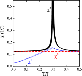
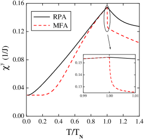
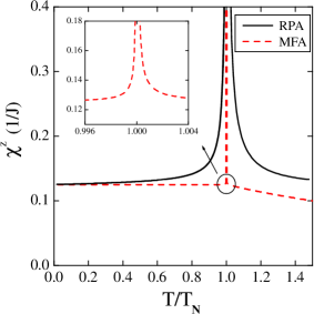
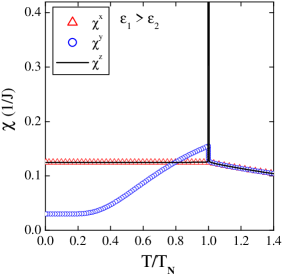
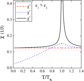
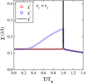
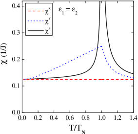
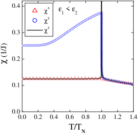
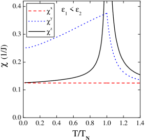
The following comments on the MFA result are in order. First, note that for physical values of d𝑑d and ΓisubscriptΓ𝑖\Gamma_{i} (d,ΓiJmuch-less-than𝑑subscriptΓ𝑖𝐽d,~{}\Gamma_{i}~{}\ll~{}J) the canting angle out of the xy𝑥𝑦xy plane is very small; thus, since the AF moment is in the yz𝑦𝑧yz plane and nearly aligned along the ±yplus-or-minus𝑦\pm y axes, χzsuperscript𝜒𝑧\chi^{z} diverges at TNMFAsubscriptsuperscript𝑇𝑀𝐹𝐴𝑁T^{MFA}_{N}, but the other two components remain finite at the transition. However, while the x𝑥x component of the susceptibility remains independent of temperature, since the canting produces a net FM moment in the z𝑧z direction that is coupled to the y𝑦y component of the local moment, there is an additional increase of χysuperscript𝜒𝑦\chi^{y} as the transition is approached from below.

Now consider the paramagnetic temperature region (T>TN𝑇subscript𝑇NT>T_{\rm N}), for which the only components with nonzero spin expectation values are those driven by the applied field. Following similar considerations to above, the final results for the components of susceptibility in the initial representation for high temperatures (T>TN𝑇subscript𝑇NT>T_{\rm N}) reads

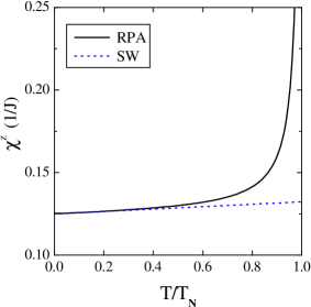
χxMFAsuperscript𝜒𝑥𝑀𝐹𝐴\displaystyle\chi^{x~{}MFA} =\displaystyle= 141J1+T,141subscript𝐽1𝑇\displaystyle\frac{1}{4}\frac{1}{J_{1}+T}, (82)
χyMFAsuperscript𝜒𝑦𝑀𝐹𝐴\displaystyle\chi^{y~{}MFA} =\displaystyle= 14sin2(θ)TJ3+14cos2(θ)T+J2,14superscript2𝜃𝑇subscript𝐽314superscript2𝜃𝑇subscript𝐽2\displaystyle\frac{1}{4}\frac{\sin^{2}(\theta)}{T-J_{3}}+\frac{1}{4}\frac{\cos^{2}(\theta)}{T+J_{2}}, (83)
χzMFAsuperscript𝜒𝑧𝑀𝐹𝐴\displaystyle\chi^{z~{}MFA} =\displaystyle= 14cos2(θ)T+J3+14sin2(θ)TJ2.14superscript2𝜃𝑇subscript𝐽314superscript2𝜃𝑇subscript𝐽2\displaystyle\frac{1}{4}\frac{\cos^{2}(\theta)}{T+J_{3}}+\frac{1}{4}\frac{\sin^{2}(\theta)}{T-J_{2}}. (84)

Note that in the limit TTNMFA=J2𝑇subscriptsuperscript𝑇𝑀𝐹𝐴Nsubscript𝐽2T\to T^{MFA}_{\rm N}=J_{2} we obtain that the x,y𝑥𝑦x,y components of the susceptibility are continuous at the transition, whereas the z𝑧z component of the susceptibility diverges at the Néel point, from above or below, owing to the presence of the weak ferromagnetic moment that first develops at the transition.

IV Linear response theory within the RPA

IV.1 Susceptibility below TNsubscript𝑇𝑁T_{N}

In this section we derive expressions for the static, uniform susceptibility within the RPA below the ordering temperature, TNsubscript𝑇𝑁T_{N}. Note that this temperature is determined with the RPA, and is not equivalent to that found in the previous section.

We employ thermal Green’s functions in the analysis of the spin Hamiltonian given in Eq. (1) with spin 1212\frac{1}{2}. The definition of such Green’s functions for two Bose operators A𝐴A, B𝐵B and the corresponding equation of motion, are given by

GAB(τ)subscript𝐺𝐴𝐵𝜏\displaystyle G_{AB}(\tau) =\displaystyle\!\!=\!\! TτA(τ)B(0),delimited-⟨⟩subscript𝑇𝜏𝐴𝜏𝐵0\displaystyle\langle T_{\tau}A(\tau)B(0)\rangle, (85)
dGAB(τ)dτdsubscript𝐺𝐴𝐵𝜏d𝜏\displaystyle\frac{{\rm d}G_{AB}(\tau)}{{\rm d}\tau} =\displaystyle\!\!=\!\! δ(τ)[A,B]+Tτ[H(τ),A(τ)]B(0).𝛿𝜏delimited-⟨⟩𝐴𝐵delimited-⟨⟩subscript𝑇𝜏𝐻𝜏𝐴𝜏𝐵0\displaystyle\delta(\tau)\langle[A,B]\rangle+\langle T_{\tau}[H(\tau),A(\tau)]B(0)\rangle. (86)

As discussed in the introduction, we adopt a procedure that was introduced by Liu,Liu as this technique allows for us to find longitudinal component of the susceptibility. To this end, we introduce the perturbed Hamiltonian (in the characteristic representation)

H1f=HCRfiσiz,subscriptsuperscript𝐻𝑓1subscript𝐻CR𝑓subscript𝑖subscriptsuperscript𝜎𝑧𝑖H^{f}_{1}=H_{\rm CR}-f\sum_{i}\sigma^{z}_{i}, (87)

where f𝑓f is a small fictitious field; note that the field is applied to the spins of sublattice 1 only, and within the present paper we restrict f𝑓f to be constant and static.

In the imaginary-time formalism, the Green’s functions to be used are

Glnf(τ)subscriptsuperscript𝐺𝑓𝑙𝑛𝜏\displaystyle G^{f}_{ln}(\tau) =\displaystyle\!\!=\!\! Tτσl+(τ)σn(0)f,superscriptdelimited-⟨⟩subscript𝑇𝜏subscriptsuperscript𝜎𝑙𝜏subscriptsuperscript𝜎𝑛0𝑓\displaystyle\langle T_{\tau}\sigma^{+}_{l}(\tau)\sigma^{-}_{n}(0)\rangle^{f},
Glnf(τ)subscriptsuperscript𝐺limit-from𝑓𝑙𝑛𝜏\displaystyle G^{f-}_{ln}(\tau) =\displaystyle\!\!=\!\! Tτσl(τ)σn(0)f,l sublattice 1,superscriptdelimited-⟨⟩subscript𝑇𝜏subscriptsuperscript𝜎𝑙𝜏subscriptsuperscript𝜎𝑛0𝑓𝑙 sublattice 1\displaystyle\langle T_{\tau}\sigma^{-}_{l}(\tau)\sigma^{-}_{n}(0)\rangle^{f},\;l\!\in\!\!\mbox{ sublattice 1},
Gnnf(τ)subscriptsuperscript𝐺𝑓superscript𝑛𝑛𝜏\displaystyle G^{f}_{n^{\prime}n}(\tau) =\displaystyle\!\!=\!\! Tτσn+(τ)σn(0)f,superscriptdelimited-⟨⟩subscript𝑇𝜏subscriptsuperscript𝜎superscript𝑛𝜏subscriptsuperscript𝜎𝑛0𝑓\displaystyle\langle T_{\tau}\sigma^{+}_{n^{\prime}}(\tau)\sigma^{-}_{n}(0)\rangle^{f},
Gnnf(τ)subscriptsuperscript𝐺limit-from𝑓superscript𝑛𝑛𝜏\displaystyle G^{f-}_{n^{\prime}n}(\tau) =\displaystyle\!\!=\!\! Tτσn(τ)σn(0)f,n sublattice 2,superscriptdelimited-⟨⟩subscript𝑇𝜏subscriptsuperscript𝜎superscript𝑛𝜏subscriptsuperscript𝜎𝑛0𝑓𝑛 sublattice 2\displaystyle\langle T_{\tau}\sigma^{-}_{n^{\prime}}(\tau)\sigma^{-}_{n}(0)\rangle^{f},\;n\!\in\!\!\mbox{ sublattice 2},

where the expectation values are taken with respect to the perturbed Hamiltonian in Eq. (87). After an expansion in a power series of f𝑓f we can write

Glnf(τ)=Gln(0)(τ)+fGln(1)(τ)+O(f2).subscriptsuperscript𝐺𝑓𝑙𝑛𝜏subscriptsuperscript𝐺0𝑙𝑛𝜏𝑓subscriptsuperscript𝐺1𝑙𝑛𝜏𝑂superscript𝑓2G^{f}_{ln}(\tau)=G^{(0)}_{ln}(\tau)+fG^{(1)}_{ln}(\tau)+O(f^{2}). (89)

Since Gln(0)(τ)=Gln(τ)subscriptsuperscript𝐺0𝑙𝑛𝜏subscript𝐺𝑙𝑛𝜏G^{(0)}_{ln}(\tau)=G_{ln}(\tau), from now drop the superscript and use

Glnf(τ)=Gln(τ)+fGln(1)(τ)+O(f2).subscriptsuperscript𝐺𝑓𝑙𝑛𝜏subscript𝐺𝑙𝑛𝜏𝑓subscriptsuperscript𝐺1𝑙𝑛𝜏𝑂superscript𝑓2G^{f}_{ln}(\tau)=G_{ln}(\tau)+fG^{(1)}_{ln}(\tau)+O(f^{2}). (90)

Also, we introduce

σiz(τ)f=σiz+fvi+O(f2),superscriptdelimited-⟨⟩subscriptsuperscript𝜎𝑧𝑖𝜏𝑓delimited-⟨⟩subscriptsuperscript𝜎𝑧𝑖𝑓subscriptv𝑖𝑂superscript𝑓2\langle\sigma^{z}_{i}(\tau)\rangle^{f}=\langle\sigma^{z}_{i}\rangle+f{\rm v}_{i}+O(f^{2}), (91)

where, due to the translation periodicity σiz=ηdelimited-⟨⟩subscriptsuperscript𝜎𝑧𝑖𝜂\langle\sigma^{z}_{i}\rangle=\eta, the order parameter at f=0𝑓0f=0.

The equation of motion for the Green’s function Glnf(τ)subscriptsuperscript𝐺𝑓𝑙𝑛𝜏G^{f}_{ln}(\tau) is given by

dGlnf(τ)dτdsubscriptsuperscript𝐺𝑓𝑙𝑛𝜏d𝜏\displaystyle\frac{{\rm d}G^{f}_{ln}(\tau)}{{\rm d}\tau} =\displaystyle\!\!=\!\! 2δ(τ)δlnσlzf2𝛿𝜏subscript𝛿𝑙𝑛superscriptdelimited-⟨⟩subscriptsuperscript𝜎𝑧𝑙𝑓\displaystyle 2\delta(\tau)\delta_{ln}\langle\sigma^{z}_{l}\rangle^{f} (92)
+\displaystyle\!\!+\!\! Tτ[HCR(τ),σl+(τ)]σn(0)ffGlnf.superscriptdelimited-⟨⟩subscript𝑇𝜏subscript𝐻CR𝜏subscriptsuperscript𝜎𝑙𝜏subscriptsuperscript𝜎𝑛0𝑓𝑓subscriptsuperscript𝐺𝑓𝑙𝑛\displaystyle\langle T_{\tau}[H_{\rm CR}(\tau),\sigma^{+}_{l}(\tau)]\sigma^{-}_{n}(0)\rangle^{f}-fG^{f}_{ln}.

In order to solve this equation for the Green’s function it must be linearized. We will use the random phase approximation (RPA), in which the fluctuations of σzsuperscript𝜎𝑧\sigma^{z} are ignored and the operator σzsuperscript𝜎𝑧\sigma^{z} is replaced by its mean value σzfsuperscriptdelimited-⟨⟩superscript𝜎𝑧𝑓\langle\sigma^{z}\rangle^{f} — this is the so-called Tyablikov’s decoupling.Tyablikov For example

Tτσlz(τ)σi+(τ)σj(0)fsuperscriptdelimited-⟨⟩subscript𝑇𝜏subscriptsuperscript𝜎𝑧𝑙𝜏subscriptsuperscript𝜎𝑖𝜏subscriptsuperscript𝜎𝑗0𝑓absent\displaystyle\langle T_{\tau}\sigma^{z}_{l}(\tau)\sigma^{+}_{i}(\tau)\sigma^{-}_{j}(0)\rangle^{f}\to
σlz(τ)fTτσi+(τ)σj(0)f=σlz(τ)fGijf(τ).absentsuperscriptdelimited-⟨⟩subscriptsuperscript𝜎𝑧𝑙𝜏𝑓superscriptdelimited-⟨⟩subscript𝑇𝜏subscriptsuperscript𝜎𝑖𝜏subscriptsuperscript𝜎𝑗0𝑓superscriptdelimited-⟨⟩subscriptsuperscript𝜎𝑧𝑙𝜏𝑓subscriptsuperscript𝐺𝑓𝑖𝑗𝜏\displaystyle\quad\to\langle\sigma^{z}_{l}(\tau)\rangle^{f}\langle T_{\tau}\sigma^{+}_{i}(\tau)\sigma^{-}_{j}(0)\rangle^{f}{=}\langle\sigma^{z}_{l}(\tau)\rangle^{f}G^{f}_{ij}(\tau). (93)

After this decoupling is introduced, Eq. (92) is found to be

dGlnf(τ)dτdsubscriptsuperscript𝐺𝑓𝑙𝑛𝜏d𝜏\displaystyle\frac{{\rm d}G^{f}_{ln}(\tau)}{{\rm d}\tau} =\displaystyle\!\!=\!\! 2δ(τ)δlnσlzfδab{2σlz(τ)f[AG(l+δ)nf(τ)BG(l+δ)nf(τ)]+J2σl+δz(τ)fGlnf(τ)}2𝛿𝜏subscript𝛿𝑙𝑛superscriptdelimited-⟨⟩subscriptsuperscript𝜎𝑧𝑙𝑓subscriptsubscript𝛿𝑎𝑏2superscriptdelimited-⟨⟩subscriptsuperscript𝜎𝑧𝑙𝜏𝑓delimited-[]𝐴subscriptsuperscript𝐺𝑓𝑙𝛿𝑛𝜏𝐵subscriptsuperscript𝐺limit-from𝑓𝑙𝛿𝑛𝜏subscript𝐽2superscriptdelimited-⟨⟩subscriptsuperscript𝜎𝑧𝑙𝛿𝜏𝑓subscriptsuperscript𝐺𝑓𝑙𝑛𝜏\displaystyle 2\delta(\tau)\delta_{ln}\langle\sigma^{z}_{l}\rangle^{f}-\sum_{\delta_{ab}}\left\{\!2\langle\sigma^{z}_{l}(\tau)\rangle^{f}[AG^{f}_{(l{+}\delta)n}(\tau){-}BG^{f-}_{(l{+}\delta)n}(\tau)]+J_{2}\langle\sigma^{z}_{l{+}\delta}(\tau)\rangle^{f}G^{f}_{ln}(\tau)\!\right\} (94)
\displaystyle\!\!-\!\!\! δac{2σlz(τ)f[AG(l+δ)nf(τ)+BG(l+δ)nf(τ)]+J2σl+δz(τ)fGlnf(τ)}fGlnf(τ),subscriptsubscript𝛿𝑎𝑐2superscriptdelimited-⟨⟩subscriptsuperscript𝜎𝑧𝑙𝜏𝑓delimited-[]𝐴subscriptsuperscript𝐺𝑓𝑙𝛿𝑛𝜏superscript𝐵subscriptsuperscript𝐺limit-from𝑓𝑙𝛿𝑛𝜏subscript𝐽2superscriptdelimited-⟨⟩subscriptsuperscript𝜎𝑧𝑙𝛿𝜏𝑓subscriptsuperscript𝐺𝑓𝑙𝑛𝜏𝑓subscriptsuperscript𝐺𝑓𝑙𝑛𝜏\displaystyle\sum_{\delta_{ac}}\left\{2\langle\sigma^{z}_{l}(\tau)\rangle^{f}[AG^{f}_{(l{+}\delta)n}(\tau){+}B^{*}G^{f-}_{(l{+}\delta)n}(\tau)]+J_{2}\langle\sigma^{z}_{l{+}\delta}(\tau)\rangle^{f}G^{f}_{ln}(\tau)\right\}-fG^{f}_{ln}(\tau),

where δabsubscriptsubscript𝛿𝑎𝑏\sum_{\delta_{ab}} refers to a summation over the nearest neighbours of the site l𝑙l in the ab𝑎𝑏ab direction, and similarly for δacsubscriptsubscript𝛿𝑎𝑐\sum_{\delta_{ac}} — see Fig. 1(b). Here, all sites l+δ𝑙𝛿l+\delta belong to the sublattice 2.

We introduce the Fourier transformation in the momentum-frequency representation for the Green’s function and the spin operator

Glnf(τ)=2Nβ𝒌,mG12f(𝒌,ωm)ei𝒌(𝐑l𝐑n)eiωmτ,subscriptsuperscript𝐺𝑓𝑙𝑛𝜏2𝑁𝛽subscript𝒌𝑚subscriptsuperscript𝐺𝑓12𝒌subscript𝜔𝑚superscriptei𝒌subscript𝐑𝑙subscript𝐑𝑛superscripteisubscript𝜔𝑚𝜏G^{f}_{ln}(\tau)=\frac{2}{N\beta}\sum_{\boldsymbol{k},m}G^{f}_{12}(\boldsymbol{k},\omega_{m}){\rm e}^{{\rm i}\boldsymbol{k}\cdot({\bf R}_{l}-{\bf R}_{n})}{\rm e}^{-{\rm i}\omega_{m}\tau}\!\!, (95)
σlz(τ)fsuperscriptdelimited-⟨⟩subscriptsuperscript𝜎𝑧𝑙𝜏𝑓\displaystyle\langle\sigma^{z}_{l}(\tau)\rangle^{f} =\displaystyle= 1β𝒌,mσ1z(𝒌,ωm)fei𝒌𝐑leiωmτ1𝛽subscript𝒌𝑚superscriptdelimited-⟨⟩subscriptsuperscript𝜎𝑧1𝒌subscript𝜔𝑚𝑓superscriptei𝒌subscript𝐑𝑙superscripteisubscript𝜔𝑚𝜏\displaystyle\frac{1}{\beta}\sum_{\boldsymbol{k},m}\langle\sigma^{z}_{1}(\boldsymbol{k},\omega_{m})\rangle^{f}{\rm e}^{-{\rm i}\boldsymbol{k}\cdot{\bf R}_{l}}{\rm e}^{-{\rm i}\omega_{m}\tau} (96)
=\displaystyle= 𝒌δ(𝒌)[η+fv1]ei𝒌𝐑l,subscript𝒌𝛿𝒌delimited-[]𝜂𝑓subscriptv1superscriptei𝒌subscript𝐑𝑙\displaystyle\sum_{\boldsymbol{k}}\delta(\boldsymbol{k})[\eta+f{\rm v}_{1}]{\rm e}^{-{\rm i}\boldsymbol{k}\cdot{\bf R}_{l}},

where the expansion in Eq. (91) and the linear response to the uniform perturbation expressed by v1(𝒌)=δ(𝒌)v1subscriptv1𝒌𝛿𝒌subscriptv1{\rm v}_{1}(\boldsymbol{k})=\delta(\boldsymbol{k}){\rm v}_{1} were taken into account. In the transformation given by Eqs. (95,96), the sum over 𝒌𝒌\boldsymbol{k} runs over 12N12𝑁\frac{1}{2}N points of the first zone in the momentum space, and ωn=2πn/βsubscript𝜔𝑛2𝜋𝑛𝛽\omega_{n}=2\pi n/\beta for n𝑛n\in\mathbb{Z} are the Bose Matsubara frequencies. Then, we can write down the equation for the Green’s function Glnf(τ)subscriptsuperscript𝐺𝑓𝑙𝑛𝜏G^{f}_{ln}(\tau) in the form

iωmG12f(𝒌,ωm)=isubscript𝜔𝑚subscriptsuperscript𝐺𝑓12𝒌subscript𝜔𝑚absent\displaystyle-{\rm i}\omega_{m}G^{f}_{12}(\boldsymbol{k},\omega_{m})= \displaystyle\!\!-\!\! fG12f(𝒌,ωm)𝑓subscriptsuperscript𝐺𝑓12𝒌subscript𝜔𝑚\displaystyle fG^{f}_{12}(\boldsymbol{k},\omega_{m}) (97)
\displaystyle\!\!-\!\! 𝒵J2[η+fv2]G12f(𝒌,ωm)𝒵subscript𝐽2delimited-[]𝜂𝑓subscriptv2subscriptsuperscript𝐺𝑓12𝒌subscript𝜔𝑚\displaystyle{\cal Z}J_{2}[\eta+f{\rm v}_{2}]G^{f}_{12}(\boldsymbol{k},\omega_{m})
\displaystyle\!\!-\!\! 2𝒵A𝒌[η+fv1]G22f(𝒌,ωm)2𝒵subscript𝐴𝒌delimited-[]𝜂𝑓subscriptv1subscriptsuperscript𝐺𝑓22𝒌subscript𝜔𝑚\displaystyle 2{\cal Z}A_{\boldsymbol{k}}[\eta+f{\rm v}_{1}]G^{f}_{22}(\boldsymbol{k},\omega_{m})
+\displaystyle\!\!+\!\! 2𝒵B𝒌[η+fv1]G22f(𝒌,ωm),2𝒵subscript𝐵𝒌delimited-[]𝜂𝑓subscriptv1subscriptsuperscript𝐺limit-from𝑓22𝒌subscript𝜔𝑚\displaystyle 2{\cal Z}B_{\boldsymbol{k}}[\eta+f{\rm v}_{1}]G^{f-}_{22}(\boldsymbol{k},\omega_{m}),

where, as before, 𝒵𝒵{\cal Z} is the coordination number, and we introduce

A𝒌=Aγ𝒌,B𝒌=(B)γ𝒌+(B)γ𝒌,formulae-sequencesubscript𝐴𝒌𝐴subscript𝛾𝒌subscript𝐵𝒌𝐵superscriptsubscript𝛾𝒌𝐵subscript𝛾𝒌\displaystyle A_{\boldsymbol{k}}=A\gamma_{\boldsymbol{k}},\quad B_{\boldsymbol{k}}=(\Re B)\gamma_{\boldsymbol{k}}^{\prime}+(\Im B)\gamma_{\boldsymbol{k}}, (98)
γ𝒌=12(coskx+cosky),γ𝒌=12(coskxcosky).formulae-sequencesubscript𝛾𝒌12subscript𝑘𝑥subscript𝑘𝑦subscriptsuperscript𝛾𝒌12subscript𝑘𝑥subscript𝑘𝑦\displaystyle\gamma_{\boldsymbol{k}}=\frac{1}{2}(\cos k_{x}+\cos k_{y}),\quad\gamma^{\prime}_{\boldsymbol{k}}=\frac{1}{2}(\cos k_{x}-\cos k_{y}).

From these we can write down the following two equations:

iωm2𝒵ηG12isubscript𝜔𝑚2𝒵𝜂subscript𝐺12\displaystyle\frac{{\rm i}\omega_{m}}{2{\cal Z}\eta}G_{12} =\displaystyle= J22G12+A𝒌G22B𝒌G22,subscript𝐽22subscript𝐺12subscript𝐴𝒌subscript𝐺22subscript𝐵𝒌subscriptsuperscript𝐺22\displaystyle\frac{J_{2}}{2}G_{12}+A_{\boldsymbol{k}}G_{22}-B_{\boldsymbol{k}}G^{-}_{22}, (99)
iωm2𝒵ηG12(1)isubscript𝜔𝑚2𝒵𝜂subscriptsuperscript𝐺112\displaystyle\frac{{\rm i}\omega_{m}}{2{\cal Z}\eta}G^{(1)}_{12} =\displaystyle= 12𝒵ηG1212𝒵𝜂subscript𝐺12\displaystyle\frac{1}{2{\cal Z}\eta}G_{12} (100)
+v2ηJ22G12+J22G12(1)+v1ηA𝒌G22+A𝒌G22(1)subscriptv2𝜂subscript𝐽22subscript𝐺12subscript𝐽22subscriptsuperscript𝐺112subscriptv1𝜂subscript𝐴𝒌subscript𝐺22subscript𝐴𝒌subscriptsuperscript𝐺122\displaystyle+\frac{{\rm v}_{2}}{\eta}\frac{J_{2}}{2}G_{12}+\frac{J_{2}}{2}G^{(1)}_{12}+\frac{{\rm v}_{1}}{\eta}A_{\boldsymbol{k}}G_{22}+A_{\boldsymbol{k}}G^{(1)}_{22}
v1ηB𝒌G22B𝒌G22(1),subscriptv1𝜂subscript𝐵𝒌subscriptsuperscript𝐺22subscript𝐵𝒌subscriptsuperscript𝐺limit-from122\displaystyle-\frac{{\rm v}_{1}}{\eta}B_{\boldsymbol{k}}G^{-}_{22}-B_{\boldsymbol{k}}G^{(1)-}_{22},

where in all equations we drop the wave vector and frequency dependencies for the Green’s functions, that is G=G(𝒌,ωm)𝐺𝐺𝒌subscript𝜔𝑚G=G(\boldsymbol{k},\omega_{m}) and G(1)=G(1)(𝒌,ωm)superscript𝐺1superscript𝐺1𝒌subscript𝜔𝑚G^{(1)}=G^{(1)}(\boldsymbol{k},\omega_{m}).

In the same way we obtain the equations of motion for the other Green’s functions (see Eq. (LABEL:eq:GGG)) within the RPA scheme. The final systems of equations for zeroth- and first-order quantities can be written as

(iωm2𝒵ηJ22)G12isubscript𝜔𝑚2𝒵𝜂subscript𝐽22subscript𝐺12\displaystyle\left(\frac{{\rm i}\omega_{m}}{2{\cal Z}\eta}-\frac{J_{2}}{2}\right)G_{12} =\displaystyle= A𝒌G22B𝒌G22,(iωm2𝒵η+J22)G12=A𝒌G22+B𝒌G22,subscript𝐴𝒌subscript𝐺22subscript𝐵𝒌subscriptsuperscript𝐺22isubscript𝜔𝑚2𝒵𝜂subscript𝐽22subscriptsuperscript𝐺12subscript𝐴𝒌subscriptsuperscript𝐺22subscriptsuperscript𝐵𝒌subscript𝐺22\displaystyle A_{\boldsymbol{k}}G_{22}-B_{\boldsymbol{k}}G^{-}_{22},\quad\qquad\left(\frac{{\rm i}\omega_{m}}{2{\cal Z}\eta}+\frac{J_{2}}{2}\right)G^{-}_{12}=-A_{\boldsymbol{k}}G^{-}_{22}+B^{*}_{\boldsymbol{k}}G_{22},
(iωm2𝒵ηJ22)G22isubscript𝜔𝑚2𝒵𝜂subscript𝐽22subscript𝐺22\displaystyle\left(\frac{{\rm i}\omega_{m}}{2{\cal Z}\eta}-\frac{J_{2}}{2}\right)G_{22} =\displaystyle= A𝒌G12B𝒌G121𝒵,(iωm2𝒵η+J22)G22=A𝒌G12+B𝒌G12;subscript𝐴𝒌subscript𝐺12subscript𝐵𝒌subscriptsuperscript𝐺121𝒵isubscript𝜔𝑚2𝒵𝜂subscript𝐽22subscriptsuperscript𝐺22subscript𝐴𝒌subscriptsuperscript𝐺12subscriptsuperscript𝐵𝒌subscript𝐺12\displaystyle A_{\boldsymbol{k}}G_{12}-B_{\boldsymbol{k}}G^{-}_{12}-\frac{1}{\cal Z},\quad\left(\frac{{\rm i}\omega_{m}}{2{\cal Z}\eta}+\frac{J_{2}}{2}\right)G^{-}_{22}=-A_{\boldsymbol{k}}G^{-}_{12}+B^{*}_{\boldsymbol{k}}G_{12};
(iωm2𝒵ηJ22)G12(1)isubscript𝜔𝑚2𝒵𝜂subscript𝐽22subscriptsuperscript𝐺112\displaystyle\left(\frac{{\rm i}\omega_{m}}{2{\cal Z}\eta}-\frac{J_{2}}{2}\right)G^{(1)}_{12} =\displaystyle= A𝒌G22(1)B𝒌G22(1)+{v2ηJ22+v1η(iωm2𝒵ηJ22)+12𝒵η}G12,subscript𝐴𝒌subscriptsuperscript𝐺122subscript𝐵𝒌subscriptsuperscript𝐺limit-from122subscriptv2𝜂subscript𝐽22subscriptv1𝜂isubscript𝜔𝑚2𝒵𝜂subscript𝐽2212𝒵𝜂subscript𝐺12\displaystyle A_{\boldsymbol{k}}G^{(1)}_{22}-B_{\boldsymbol{k}}G^{(1)-}_{22}+\bigg{\{}\frac{{\rm v}_{2}}{\eta}\frac{J_{2}}{2}+\frac{{\rm v}_{1}}{\eta}\bigg{(}\frac{{\rm i}\omega_{m}}{2{\cal Z}\eta}-\frac{J_{2}}{2}\bigg{)}+\frac{1}{2{\cal Z}\eta}\bigg{\}}G_{12},
(iωm2𝒵ηJ22)G22(1)isubscript𝜔𝑚2𝒵𝜂subscript𝐽22subscriptsuperscript𝐺122\displaystyle\left(\frac{{\rm i}\omega_{m}}{2{\cal Z}\eta}-\frac{J_{2}}{2}\right)G^{(1)}_{22} =\displaystyle= A𝒌G12(1)B𝒌G12(1)+{v1ηJ22+v2η(iωm2𝒵ηJ22)}G22,subscript𝐴𝒌subscriptsuperscript𝐺112subscript𝐵𝒌subscriptsuperscript𝐺limit-from112subscriptv1𝜂subscript𝐽22subscriptv2𝜂isubscript𝜔𝑚2𝒵𝜂subscript𝐽22subscript𝐺22\displaystyle A_{\boldsymbol{k}}G^{(1)}_{12}-B_{\boldsymbol{k}}G^{(1)-}_{12}+\bigg{\{}\frac{{\rm v}_{1}}{\eta}\frac{J_{2}}{2}+\frac{{\rm v}_{2}}{\eta}\bigg{(}\frac{{\rm i}\omega_{m}}{2{\cal Z}\eta}-\frac{J_{2}}{2}\bigg{)}\bigg{\}}G_{22},
(iωm2𝒵η+J22)G12(1)isubscript𝜔𝑚2𝒵𝜂subscript𝐽22subscriptsuperscript𝐺limit-from112\displaystyle\left(\frac{{\rm i}\omega_{m}}{2{\cal Z}\eta}+\frac{J_{2}}{2}\right)G^{(1)-}_{12} =\displaystyle= A𝒌G22(1)+B𝒌G22(1){v2ηJ22v1η(iωm2𝒵η+J22)+12𝒵η}G12,subscript𝐴𝒌subscriptsuperscript𝐺limit-from122subscriptsuperscript𝐵𝒌subscriptsuperscript𝐺122subscriptv2𝜂subscript𝐽22subscriptv1𝜂isubscript𝜔𝑚2𝒵𝜂subscript𝐽2212𝒵𝜂subscriptsuperscript𝐺12\displaystyle-A_{\boldsymbol{k}}G^{(1)-}_{22}+B^{*}_{\boldsymbol{k}}G^{(1)}_{22}-\bigg{\{}\frac{{\rm v}_{2}}{\eta}\frac{J_{2}}{2}-\frac{{\rm v}_{1}}{\eta}\bigg{(}\frac{{\rm i}\omega_{m}}{2{\cal Z}\eta}+\frac{J_{2}}{2}\bigg{)}+\frac{1}{2{\cal Z}\eta}\bigg{\}}G^{-}_{12},
(iωm2𝒵η+J22)G22(1)isubscript𝜔𝑚2𝒵𝜂subscript𝐽22subscriptsuperscript𝐺limit-from122\displaystyle\left(\frac{{\rm i}\omega_{m}}{2{\cal Z}\eta}+\frac{J_{2}}{2}\right)G^{(1)-}_{22} =\displaystyle= A𝒌G12(1)+B𝒌G12(1){v1ηJ22v2η(iωm2𝒵η+J22)}G22;subscript𝐴𝒌subscriptsuperscript𝐺limit-from112subscriptsuperscript𝐵𝒌subscriptsuperscript𝐺112subscriptv1𝜂subscript𝐽22subscriptv2𝜂isubscript𝜔𝑚2𝒵𝜂subscript𝐽22subscriptsuperscript𝐺22\displaystyle-A_{\boldsymbol{k}}G^{(1)-}_{12}+B^{*}_{\boldsymbol{k}}G^{(1)}_{12}-\bigg{\{}\frac{{\rm v}_{1}}{\eta}\frac{J_{2}}{2}-\frac{{\rm v}_{2}}{\eta}\bigg{(}\frac{{\rm i}\omega_{m}}{2{\cal Z}\eta}+\frac{J_{2}}{2}\bigg{)}\bigg{\}}G^{-}_{22};
(iωm2𝒵ηJ22)G21(1)isubscript𝜔𝑚2𝒵𝜂subscript𝐽22subscriptsuperscript𝐺121\displaystyle\left(\frac{{\rm i}\omega_{m}}{2{\cal Z}\eta}-\frac{J_{2}}{2}\right)G^{(1)}_{21} =\displaystyle= A𝒌G11(1)B𝒌G11(1)+{v1ηJ22+v2η(iωm2𝒵ηJ22)}G12,subscript𝐴𝒌subscriptsuperscript𝐺111subscript𝐵𝒌subscriptsuperscript𝐺limit-from111subscriptv1𝜂subscript𝐽22subscriptv2𝜂isubscript𝜔𝑚2𝒵𝜂subscript𝐽22subscript𝐺12\displaystyle A_{\boldsymbol{k}}G^{(1)}_{11}-B_{\boldsymbol{k}}G^{(1)-}_{11}+\bigg{\{}\frac{{\rm v}_{1}}{\eta}\frac{J_{2}}{2}+\frac{{\rm v}_{2}}{\eta}\bigg{(}\frac{{\rm i}\omega_{m}}{2{\cal Z}\eta}-\frac{J_{2}}{2}\bigg{)}\bigg{\}}G_{12},
(iωm2𝒵ηJ22)G11(1)isubscript𝜔𝑚2𝒵𝜂subscript𝐽22subscriptsuperscript𝐺111\displaystyle\left(\frac{{\rm i}\omega_{m}}{2{\cal Z}\eta}-\frac{J_{2}}{2}\right)G^{(1)}_{11} =\displaystyle= A𝒌G21(1)B𝒌G21(1)+{v2ηJ22+v1η(iωm2𝒵ηJ22)+12𝒵η}G22,subscript𝐴𝒌subscriptsuperscript𝐺121subscript𝐵𝒌subscriptsuperscript𝐺limit-from121subscriptv2𝜂subscript𝐽22subscriptv1𝜂isubscript𝜔𝑚2𝒵𝜂subscript𝐽2212𝒵𝜂subscript𝐺22\displaystyle A_{\boldsymbol{k}}G^{(1)}_{21}-B_{\boldsymbol{k}}G^{(1)-}_{21}+\bigg{\{}\frac{{\rm v}_{2}}{\eta}\frac{J_{2}}{2}+\frac{{\rm v}_{1}}{\eta}\bigg{(}\frac{{\rm i}\omega_{m}}{2{\cal Z}\eta}-\frac{J_{2}}{2}\bigg{)}+\frac{1}{2{\cal Z}\eta}\bigg{\}}G_{22},
(iωm2𝒵η+J22)G21(1)isubscript𝜔𝑚2𝒵𝜂subscript𝐽22subscriptsuperscript𝐺limit-from121\displaystyle\left(\frac{{\rm i}\omega_{m}}{2{\cal Z}\eta}+\frac{J_{2}}{2}\right)G^{(1)-}_{21} =\displaystyle= A𝒌G11(1)+B𝒌G11(1){v1ηJ22v2η(iωm2𝒵η+J22)}G12,subscript𝐴𝒌subscriptsuperscript𝐺limit-from111subscriptsuperscript𝐵𝒌subscriptsuperscript𝐺111subscriptv1𝜂subscript𝐽22subscriptv2𝜂isubscript𝜔𝑚2𝒵𝜂subscript𝐽22subscriptsuperscript𝐺12\displaystyle-A_{\boldsymbol{k}}G^{(1)-}_{11}+B^{*}_{\boldsymbol{k}}G^{(1)}_{11}-\bigg{\{}\frac{{\rm v}_{1}}{\eta}\frac{J_{2}}{2}-\frac{{\rm v}_{2}}{\eta}\bigg{(}\frac{{\rm i}\omega_{m}}{2{\cal Z}\eta}+\frac{J_{2}}{2}\bigg{)}\bigg{\}}G^{-}_{12},
(iωm2𝒵η+J22)G11(1)isubscript𝜔𝑚2𝒵𝜂subscript𝐽22subscriptsuperscript𝐺limit-from111\displaystyle\left(\frac{{\rm i}\omega_{m}}{2{\cal Z}\eta}+\frac{J_{2}}{2}\right)G^{(1)-}_{11} =\displaystyle= A𝒌G21(1)+B𝒌G21(1){v2ηJ22v1η(iωm2𝒵η+J22)+12𝒵η}G22,subscript𝐴𝒌subscriptsuperscript𝐺limit-from121subscriptsuperscript𝐵𝒌subscriptsuperscript𝐺121subscriptv2𝜂subscript𝐽22subscriptv1𝜂isubscript𝜔𝑚2𝒵𝜂subscript𝐽2212𝒵𝜂subscriptsuperscript𝐺22\displaystyle-A_{\boldsymbol{k}}G^{(1)-}_{21}+B^{*}_{\boldsymbol{k}}G^{(1)}_{21}-\bigg{\{}\frac{{\rm v}_{2}}{\eta}\frac{J_{2}}{2}-\frac{{\rm v}_{1}}{\eta}\bigg{(}\frac{{\rm i}\omega_{m}}{2{\cal Z}\eta}+\frac{J_{2}}{2}\bigg{)}+\frac{1}{2{\cal Z}\eta}\bigg{\}}G^{-}_{22},
(103)

where we have taken into account the relations

G12=G21,G11=G22,formulae-sequencesubscript𝐺12subscript𝐺21subscript𝐺11subscript𝐺22\displaystyle G_{12}=G_{21},\quad G_{11}=G_{22},
G12=G21,G11=G22.formulae-sequencesubscriptsuperscript𝐺12subscriptsuperscript𝐺21subscriptsuperscript𝐺11subscriptsuperscript𝐺22\displaystyle G^{-}_{12}=G^{-}_{21},\quad G^{-}_{11}=G^{-}_{22}. (104)

The poles of the zero-order Green’s functions G𝐺G have to be the same as the poles found for the first-order ones G(1)superscript𝐺1G^{(1)}. This can be seen directly by comparing the structure of the systems of equations for the corresponding quantities: the system in Eq. (LABEL:eq:Z_eq) for the zero-order functions is identical with the systems in Eqs. (LABEL:eq:F_eq,103) for the first-order ones, except for the free terms. The free terms in the first-order systems are determined by the zero-order Green’s functions, thus, the first-order quantities G(1)superscript𝐺1G^{(1)} can be written down in terms of the solution for the zero-order system of Eq. (LABEL:eq:Z_eq), and the as yet unknown quantities v1subscriptv1{\rm v}_{1} and v2subscriptv2{\rm v}_{2}.

To calculate v1,2subscriptv12{\rm v}_{1,2} we use a relation connecting vv{\rm v} and the Green’s functions G(1)(𝒌,0)superscript𝐺1𝒌superscript0G^{(1)}(\boldsymbol{k},0^{-}). From the definitions in Eq. (LABEL:eq:GGG) and the expansion in Eq. (91) we have

Giif(0)=12σizf=12ηfvi,subscriptsuperscript𝐺𝑓𝑖𝑖superscript012superscriptdelimited-⟨⟩subscriptsuperscript𝜎𝑧𝑖𝑓12𝜂𝑓subscriptv𝑖\displaystyle G^{f}_{ii}(0^{-})=\frac{1}{2}-\langle\sigma^{z}_{i}\rangle^{f}=\frac{1}{2}-\eta-f{\rm v}_{i}, (105)

while the expansion in Eq. (90) leads to

Giif(0)=Gii(0)+fGii(1)(0)=12η+fGii(1)(0).subscriptsuperscript𝐺𝑓𝑖𝑖superscript0subscript𝐺𝑖𝑖superscript0𝑓subscriptsuperscript𝐺1𝑖𝑖superscript012𝜂𝑓subscriptsuperscript𝐺1𝑖𝑖superscript0G^{f}_{ii}(0^{-})=G_{ii}(0^{-})+fG^{(1)}_{ii}(0^{-})=\frac{1}{2}-\eta+fG^{(1)}_{ii}(0^{-}). (106)

Thus, we can write down vi=Gii(1)(0)subscriptv𝑖subscriptsuperscript𝐺1𝑖𝑖superscript0-{\rm v}_{i}=G^{(1)}_{ii}(0^{-}), and after Fourier summation one obtains

v1subscriptv1\displaystyle-{\rm v}_{1} =\displaystyle= 2N𝒌G11(1)(𝒌,0),2𝑁subscript𝒌subscriptsuperscript𝐺111𝒌superscript0\displaystyle\frac{2}{N}\sum_{\boldsymbol{k}}G^{(1)}_{11}(\boldsymbol{k},0^{-}), (107)
v2subscriptv2\displaystyle-{\rm v}_{2} =\displaystyle= 2N𝒌G22(1)(𝒌,0).2𝑁subscript𝒌subscriptsuperscript𝐺122𝒌superscript0\displaystyle\frac{2}{N}\sum_{\boldsymbol{k}}G^{(1)}_{22}(\boldsymbol{k},0^{-}). (108)

The solution of the system in Eq. (LABEL:eq:F_eq) gives us the first-order Green’s function G22(1)(𝒌,ωm)subscriptsuperscript𝐺122𝒌subscript𝜔𝑚G^{(1)}_{22}(\boldsymbol{k},\omega_{m}) and therefore v2subscriptv2{\rm v}_{2}. Similarly, to find v1subscriptv1{\rm v}_{1} we use Eq. (103).

The solution of the system of equations in Eq. (LABEL:eq:Z_eq) for the zeroth-order Green’s functions turns out to be

G12(𝒌,ωn)=subscript𝐺12𝒌subscript𝜔𝑛absent\displaystyle G_{12}(\boldsymbol{k},\omega_{n})= η2{(1+J2/2+A𝒌ω1(𝒌))1iωnε1(𝒌)+(1J2/2+A𝒌ω1(𝒌))1iωn+ε1(𝒌)\displaystyle\!\!\!\!\!-\frac{\eta}{2}\left\{\left(1+\frac{J_{2}/2{+}A_{\boldsymbol{k}}}{\omega_{1}(\boldsymbol{k})}\right)\frac{1}{{\rm i}\omega_{n}{-}\varepsilon_{1}(\boldsymbol{k})}+\left(1-\frac{J_{2}/2{+}A_{\boldsymbol{k}}}{\omega_{1}(\boldsymbol{k})}\right)\frac{1}{{\rm i}\omega_{n}{+}\varepsilon_{1}(\boldsymbol{k})}\right.
(1+J2/2A𝒌ω2(𝒌))1iωnε2(𝒌)(1J2/2A𝒌ω2(𝒌))1iωn+ε2(𝒌)},\displaystyle\left.\quad-\left(1+\frac{J_{2}/2{-}A_{\boldsymbol{k}}}{\omega_{2}(\boldsymbol{k})}\right)\frac{1}{{\rm i}\omega_{n}{-}\varepsilon_{2}(\boldsymbol{k})}-\left(1-\frac{J_{2}/2{-}A_{\boldsymbol{k}}}{\omega_{2}(\boldsymbol{k})}\right)\frac{1}{{\rm i}\omega_{n}{+}\varepsilon_{2}(\boldsymbol{k})}\right\},
G22(𝒌,ωn)=subscript𝐺22𝒌subscript𝜔𝑛absent\displaystyle G_{22}(\boldsymbol{k},\omega_{n})= η2{(1+J2/2+A𝒌ω1(𝒌))1iωnε1(𝒌)+(1J2/2+A𝒌ω1(𝒌))1iωn+ε1(𝒌)\displaystyle\!\!\!\!\!-\frac{\eta}{2}\left\{\left(1+\frac{J_{2}/2{+}A_{\boldsymbol{k}}}{\omega_{1}(\boldsymbol{k})}\right)\frac{1}{{\rm i}\omega_{n}{-}\varepsilon_{1}(\boldsymbol{k})}+\left(1-\frac{J_{2}/2{+}A_{\boldsymbol{k}}}{\omega_{1}(\boldsymbol{k})}\right)\frac{1}{{\rm i}\omega_{n}{+}\varepsilon_{1}(\boldsymbol{k})}\right.
+(1+J2/2A𝒌ω2(𝒌))1iωnε2(𝒌)+(1J2/2A𝒌ω2(𝒌))1iωn+ε2(𝒌)},\displaystyle\left.\quad+\left(1+\frac{J_{2}/2{-}A_{\boldsymbol{k}}}{\omega_{2}(\boldsymbol{k})}\right)\frac{1}{{\rm i}\omega_{n}{-}\varepsilon_{2}(\boldsymbol{k})}+\left(1-\frac{J_{2}/2{-}A_{\boldsymbol{k}}}{\omega_{2}(\boldsymbol{k})}\right)\frac{1}{{\rm i}\omega_{n}{+}\varepsilon_{2}(\boldsymbol{k})}\right\},
G12(𝒌,ωn)=subscriptsuperscript𝐺12𝒌subscript𝜔𝑛absent\displaystyle G^{-}_{12}(\boldsymbol{k},\omega_{n})= η2B𝒌{1ω1(𝒌)(1iωnε1(𝒌)1iωn+ε1(𝒌))+1ω2(𝒌)(1iωnε2(𝒌)1iωn+ε2(𝒌))},𝜂2subscriptsuperscript𝐵𝒌1subscript𝜔1𝒌1isubscript𝜔𝑛subscript𝜀1𝒌1isubscript𝜔𝑛subscript𝜀1𝒌1subscript𝜔2𝒌1isubscript𝜔𝑛subscript𝜀2𝒌1isubscript𝜔𝑛subscript𝜀2𝒌\displaystyle\!\!\!\!\!-\frac{\eta}{2}B^{*}_{\boldsymbol{k}}\left\{\!\frac{1}{\omega_{1}(\boldsymbol{k})}\left(\frac{1}{{\rm i}\omega_{n}{-}\varepsilon_{1}(\boldsymbol{k})}-\frac{1}{{\rm i}\omega_{n}{+}\varepsilon_{1}(\boldsymbol{k})}\right)+\frac{1}{\omega_{2}(\boldsymbol{k})}\left(\frac{1}{{\rm i}\omega_{n}{-}\varepsilon_{2}(\boldsymbol{k})}-\frac{1}{{\rm i}\omega_{n}{+}\varepsilon_{2}(\boldsymbol{k})}\right)\!\right\},
G22(𝒌,ωn)=subscriptsuperscript𝐺22𝒌subscript𝜔𝑛absent\displaystyle G^{-}_{22}(\boldsymbol{k},\omega_{n})= η2B𝒌{1ω1(𝒌)(1iωnε1(𝒌)1iωn+ε1(𝒌))1ω2(𝒌)(1iωnε2(𝒌)1iωn+ε2(𝒌))},𝜂2subscriptsuperscript𝐵𝒌1subscript𝜔1𝒌1isubscript𝜔𝑛subscript𝜀1𝒌1isubscript𝜔𝑛subscript𝜀1𝒌1subscript𝜔2𝒌1isubscript𝜔𝑛subscript𝜀2𝒌1isubscript𝜔𝑛subscript𝜀2𝒌\displaystyle\!\!\!\!\!-\frac{\eta}{2}B^{*}_{\boldsymbol{k}}\left\{\!\frac{1}{\omega_{1}(\boldsymbol{k})}\left(\frac{1}{{\rm i}\omega_{n}{-}\varepsilon_{1}(\boldsymbol{k})}-\frac{1}{{\rm i}\omega_{n}{+}\varepsilon_{1}(\boldsymbol{k})}\right)-\frac{1}{\omega_{2}(\boldsymbol{k})}\left(\frac{1}{{\rm i}\omega_{n}{-}\varepsilon_{2}(\boldsymbol{k})}-\frac{1}{{\rm i}\omega_{n}{+}\varepsilon_{2}(\boldsymbol{k})}\right)\!\right\},

where the spectra for the out-of-plane ε1(𝒌)subscript𝜀1𝒌\varepsilon_{1}(\boldsymbol{k}) and in-plane ε2(𝒌)subscript𝜀2𝒌\varepsilon_{2}(\boldsymbol{k}) modesKoshibae are given by

ε1(𝒌)=2𝒵ηω1(𝒌)=2𝒵η(J2/2+A𝒌)2|B𝒌|2,subscript𝜀1𝒌2𝒵𝜂subscript𝜔1𝒌2𝒵𝜂superscriptsubscript𝐽22subscript𝐴𝒌2superscriptsubscript𝐵𝒌2\displaystyle\varepsilon_{1}(\boldsymbol{k})=2{\cal Z}\eta\omega_{1}(\boldsymbol{k})=2{\cal Z}\eta\sqrt{(J_{2}/2+A_{\boldsymbol{k}})^{2}-|B_{\boldsymbol{k}}|^{2}},
ε2(𝒌)=2𝒵ηω2(𝒌)=2𝒵η(J2/2A𝒌)2|B𝒌|2.subscript𝜀2𝒌2𝒵𝜂subscript𝜔2𝒌2𝒵𝜂superscriptsubscript𝐽22subscript𝐴𝒌2superscriptsubscript𝐵𝒌2\displaystyle\varepsilon_{2}(\boldsymbol{k})=2{\cal Z}\eta\omega_{2}(\boldsymbol{k})=2{\cal Z}\eta\sqrt{(J_{2}/2-A_{\boldsymbol{k}})^{2}-|B_{\boldsymbol{k}}|^{2}}.
(110)

After the substitution of the results in Eq. (LABEL:eq:G_sol) into the system of equations in Eqs. (LABEL:eq:F_eq,103), and then using the solutions for G11(1)(𝒌,ωm)subscriptsuperscript𝐺111𝒌subscript𝜔𝑚G^{(1)}_{11}(\boldsymbol{k},\omega_{m}), G22(1)(𝒌,ωm)subscriptsuperscript𝐺122𝒌subscript𝜔𝑚G^{(1)}_{22}(\boldsymbol{k},\omega_{m}), the results for quantities v1subscriptv1{\rm v}_{1} and v2subscriptv2{\rm v}_{2} are found to be

v1v2subscriptv1subscriptv2\displaystyle{\rm v}_{1}-{\rm v}_{2} =\displaystyle= η2C11+4η2J2C1,superscript𝜂2subscript𝐶114superscript𝜂2subscript𝐽2subscript𝐶1\displaystyle\frac{\eta^{2}C_{1}}{1+4\eta^{2}J_{2}C_{1}}, (111)
v1+v2subscriptv1subscriptv2\displaystyle{\rm v}_{1}+{\rm v}_{2} =\displaystyle= η2C218η2C3,superscript𝜂2subscript𝐶218superscript𝜂2subscript𝐶3\displaystyle\frac{\eta^{2}C_{2}}{1-8\eta^{2}C_{3}}, (112)

where

C1subscript𝐶1\displaystyle C_{1} =\displaystyle= 2N𝒌2{(1+(J2/2)2A𝒌2|B𝒌|2ω1(𝒌)ω2(𝒌))n(ε1)n(ε2)ε2(𝒌)ε1(𝒌)(1(J2/2)2A𝒌2|B𝒌|2ω1(𝒌)ω2(𝒌))n(ε1)+n(ε2)+1ε1(𝒌)+ε2(𝒌)},2𝑁subscript𝒌21superscriptsubscript𝐽222superscriptsubscript𝐴𝒌2superscriptsubscript𝐵𝒌2subscript𝜔1𝒌subscript𝜔2𝒌𝑛subscript𝜀1𝑛subscript𝜀2subscript𝜀2𝒌subscript𝜀1𝒌1superscriptsubscript𝐽222superscriptsubscript𝐴𝒌2superscriptsubscript𝐵𝒌2subscript𝜔1𝒌subscript𝜔2𝒌𝑛subscript𝜀1𝑛subscript𝜀21subscript𝜀1𝒌subscript𝜀2𝒌\displaystyle\frac{2}{N}\sum_{\boldsymbol{k}}2\left\{\left(1+\frac{(J_{2}/2)^{2}{-}A_{\boldsymbol{k}}^{2}{-}|B_{\boldsymbol{k}}|^{2}}{\omega_{1}(\boldsymbol{k})\omega_{2}(\boldsymbol{k})}\right)\frac{n(\varepsilon_{1}){-}n(\varepsilon_{2})}{\varepsilon_{2}(\boldsymbol{k}){-}\varepsilon_{1}(\boldsymbol{k})}-\left(1-\frac{(J_{2}/2)^{2}{-}A_{\boldsymbol{k}}^{2}{-}|B_{\boldsymbol{k}}|^{2}}{\omega_{1}(\boldsymbol{k})\omega_{2}(\boldsymbol{k})}\right)\frac{n(\varepsilon_{1}){+}n(\varepsilon_{2}){+}1}{\varepsilon_{1}(\boldsymbol{k})+\varepsilon_{2}(\boldsymbol{k})}\right\},
C2subscript𝐶2\displaystyle C_{2} =\displaystyle= 2N𝒌{(J2/2+A𝒌)2β/2ω12(𝒌)sinh2βε12+|B𝒌|2[2n(ε1)+1]ω12(𝒌)ε1(𝒌)+(J2/2A𝒌)2β/2ω22(𝒌)sinh2βε22+|B𝒌|2[2n(ε2)+1]ω22(𝒌)ε2(𝒌)},2𝑁subscript𝒌superscriptsubscript𝐽22subscript𝐴𝒌2𝛽2subscriptsuperscript𝜔21𝒌superscript2𝛽subscript𝜀12superscriptsubscript𝐵𝒌2delimited-[]2𝑛subscript𝜀11subscriptsuperscript𝜔21𝒌subscript𝜀1𝒌superscriptsubscript𝐽22subscript𝐴𝒌2𝛽2subscriptsuperscript𝜔22𝒌superscript2𝛽subscript𝜀22superscriptsubscript𝐵𝒌2delimited-[]2𝑛subscript𝜀21subscriptsuperscript𝜔22𝒌subscript𝜀2𝒌\displaystyle\frac{2}{N}\sum_{\boldsymbol{k}}\left\{\!\frac{(J_{2}/2{+}A_{\boldsymbol{k}})^{2}\beta/2}{\omega^{2}_{1}(\boldsymbol{k})\sinh^{2}\frac{\beta\varepsilon_{1}}{2}}+\frac{|B_{\boldsymbol{k}}|^{2}[2n(\varepsilon_{1}){+}1]}{\omega^{2}_{1}(\boldsymbol{k})\varepsilon_{1}(\boldsymbol{k})}+\frac{(J_{2}/2{-}A_{\boldsymbol{k}})^{2}\beta/2}{\omega^{2}_{2}(\boldsymbol{k})\sinh^{2}\frac{\beta\varepsilon_{2}}{2}}+\frac{|B_{\boldsymbol{k}}|^{2}[2n(\varepsilon_{2}){+}1]}{\omega^{2}_{2}(\boldsymbol{k})\varepsilon_{2}(\boldsymbol{k})}\!\right\},
C3subscript𝐶3\displaystyle C_{3} =\displaystyle= 2N𝒌{(J2/2+A𝒌)β/2sinh2βε12+(J2/2A𝒌)β/2sinh2βε22},heren(ε1,2)=[exp(βε1,2(𝒌))1]1.2𝑁subscript𝒌subscript𝐽22subscript𝐴𝒌𝛽2superscript2𝛽subscript𝜀12subscript𝐽22subscript𝐴𝒌𝛽2superscript2𝛽subscript𝜀22here𝑛subscript𝜀12superscriptdelimited-[]exp𝛽subscript𝜀12𝒌11\displaystyle\frac{2}{N}\sum_{\boldsymbol{k}}\left\{\!\frac{(J_{2}/2{+}A_{\boldsymbol{k}})\beta/2}{\sinh^{2}\frac{\beta\varepsilon_{1}}{2}}+\frac{(J_{2}/2{-}A_{\boldsymbol{k}})\beta/2}{\sinh^{2}\frac{\beta\varepsilon_{2}}{2}}\!\right\},\quad\mbox{here}\;\;n(\varepsilon_{1,2})=[{\rm exp}(\beta\varepsilon_{1,2}(\boldsymbol{k}))-1]^{-1}.

Now let us find the quantities which determine a linear response to a magnetic field applied to the one of sublattice – see Eqs. (59,60). The longitudinal z𝑧z components of the susceptibility in the characteristic representation are given by

χ11σzσz=σ1zff|f=0=v1,χ12σzσz=σ2zff|f=0=v2,formulae-sequencesubscriptsuperscript𝜒superscript𝜎𝑧superscript𝜎𝑧11evaluated-atsuperscriptdelimited-⟨⟩subscriptsuperscript𝜎𝑧1𝑓𝑓𝑓0subscriptv1subscriptsuperscript𝜒superscript𝜎𝑧superscript𝜎𝑧12evaluated-atsuperscriptdelimited-⟨⟩subscriptsuperscript𝜎𝑧2𝑓𝑓𝑓0subscriptv2\chi^{\sigma^{z}\sigma^{z}}_{11}=\frac{\partial\langle\sigma^{z}_{1}\rangle^{f}}{\partial f}\Big{|}_{f=0}={\rm v}_{1},\;\;\;\chi^{\sigma^{z}\sigma^{z}}_{12}=\frac{\partial\langle\sigma^{z}_{2}\rangle^{f}}{\partial f}\Big{|}_{f=0}={\rm v}_{2}, (114)

where the expansion of Eq. (91) was used. The transverse x𝑥x and y𝑦y components of the susceptibility tensor are determined in the terms of Green’s functions as

χ11σασαsubscriptsuperscript𝜒superscript𝜎𝛼superscript𝜎superscript𝛼11\displaystyle\chi^{\sigma^{\alpha}\sigma^{\alpha^{\prime}}}_{11} =\displaystyle= 2Ni,i0βTτσiα(τ)σiα(0)dτ,2𝑁subscript𝑖superscript𝑖subscriptsuperscript𝛽0delimited-⟨⟩subscript𝑇𝜏superscriptsubscript𝜎𝑖𝛼𝜏superscriptsubscript𝜎superscript𝑖superscript𝛼0differential-d𝜏\displaystyle\frac{2}{N}\sum_{i,i^{\prime}}\int^{\beta}_{0}\!\!\langle T_{\tau}\sigma_{i}^{\alpha}(\tau)\sigma_{i^{\prime}}^{\alpha^{\prime}}(0)\rangle{\rm d}\tau,
χ12σασαsubscriptsuperscript𝜒superscript𝜎𝛼superscript𝜎superscript𝛼12\displaystyle\chi^{\sigma^{\alpha}\sigma^{\alpha^{\prime}}}_{12} =\displaystyle= 2Ni,j0βTτσiα(τ)σjα(0)dτ,2𝑁subscript𝑖𝑗subscriptsuperscript𝛽0delimited-⟨⟩subscript𝑇𝜏superscriptsubscript𝜎𝑖𝛼𝜏superscriptsubscript𝜎𝑗superscript𝛼0differential-d𝜏\displaystyle\frac{2}{N}\sum_{i,j}\int^{\beta}_{0}\!\!\langle T_{\tau}\sigma_{i}^{\alpha}(\tau)\sigma_{j}^{\alpha^{\prime}}(0)\rangle{\rm d}\tau,

where α=x,y𝛼𝑥𝑦\alpha=x,y. By substituting the solutions in Eq. (LABEL:eq:G_sol) into the definition in Eq. (LABEL:eq:def) for the transverse components of susceptibility, we easily obtain exactly the same result that we have already found within our MFA calculations – that is, Eq. (LABEL:eq:all_chi_sigma).

Then, using Eqs. (61)-(63) the components of the susceptibility in the initial coordinate system of Eq. (1) are found to be

χxsuperscript𝜒𝑥\displaystyle\chi^{x} =\displaystyle= 141J1+J2,141subscript𝐽1subscript𝐽2\displaystyle\frac{1}{4}\frac{1}{J_{1}+J_{2}}, (116)
χysuperscript𝜒𝑦\displaystyle\chi^{y} =\displaystyle= 14sin2(θ)J2J3+cos2(θ)[v1v2],14superscript2𝜃subscript𝐽2subscript𝐽3superscript2𝜃delimited-[]subscriptv1subscriptv2\displaystyle\frac{1}{4}\frac{\sin^{2}(\theta)}{J_{2}-J_{3}}+\cos^{2}(\theta)[{\rm v}_{1}-{\rm v}_{2}], (117)
χzsuperscript𝜒𝑧\displaystyle\chi^{z} =\displaystyle= 14cos2(θ)J2+J3+sin2(θ)[v1+v2].14superscript2𝜃subscript𝐽2subscript𝐽3superscript2𝜃delimited-[]subscriptv1subscriptv2\displaystyle\frac{1}{4}\frac{\cos^{2}(\theta)}{J_{2}+J_{3}}+\sin^{2}(\theta)[{\rm v}_{1}+{\rm v}_{2}]. (118)

For completeness, we mention that we have also performed the theoretical investigation of this model (1) within spin-wave (SW) theory, and the final result for the components of static susceptibility turns out to be

χxSWsuperscript𝜒𝑥𝑆𝑊\displaystyle\chi^{x~{}SW} =\displaystyle= 141J1+J2,141subscript𝐽1subscript𝐽2\displaystyle\frac{1}{4}\frac{1}{J_{1}+J_{2}}, (119)
χySWsuperscript𝜒𝑦𝑆𝑊\displaystyle\chi^{y~{}SW} =\displaystyle= 14sin2(θ)J2J3+cos2(θ)S2C1|ηS,14superscript2𝜃subscript𝐽2subscript𝐽3evaluated-atsuperscript2𝜃superscript𝑆2subscript𝐶1𝜂𝑆\displaystyle\frac{1}{4}\frac{\sin^{2}(\theta)}{J_{2}-J_{3}}+\cos^{2}(\theta)S^{2}C_{1}\big{|}_{\eta\to S}, (120)
χzSWsuperscript𝜒𝑧𝑆𝑊\displaystyle\chi^{z~{}SW} =\displaystyle= 14cos2(θ)J2+J3+sin2(θ)S2C2|ηS.14superscript2𝜃subscript𝐽2subscript𝐽3evaluated-atsuperscript2𝜃superscript𝑆2subscript𝐶2𝜂𝑆\displaystyle\frac{1}{4}\frac{\cos^{2}(\theta)}{J_{2}+J_{3}}+\sin^{2}(\theta)S^{2}C_{2}\big{|}_{\eta\to S}. (121)

It can be noted that the difference in the results within the RPA, Eqs. (116)-(118), and spin-wave theory, Eqs. (119)-(121), came from the calculation of the components of the susceptibility in the direction of the sublattice magnetization (that is χ11σzσzsubscriptsuperscript𝜒superscript𝜎𝑧superscript𝜎𝑧11\chi^{\sigma^{z}\sigma^{z}}_{11} and χ12σzσzsubscriptsuperscript𝜒superscript𝜎𝑧superscript𝜎𝑧12\chi^{\sigma^{z}\sigma^{z}}_{12}). The spin-wave theory gives unity in the denominator of the expressions for χ11σzσzsubscriptsuperscript𝜒superscript𝜎𝑧superscript𝜎𝑧11\chi^{\sigma^{z}\sigma^{z}}_{11} and χ12σzσzsubscriptsuperscript𝜒superscript𝜎𝑧superscript𝜎𝑧12\chi^{\sigma^{z}\sigma^{z}}_{12} in Eq. (111), and S=1/2𝑆12S=1/2 instead of the order parameter η𝜂\eta everywhere in the numerator. The similar situation takes place for antiferromagnetic Heisenberg model within the RPA schemeLiu and spin-wave theory.Liu2

We also mention that the transverse components of the susceptibility in the characteristic representation (LABEL:eq:all_chi_sigma) are equal within the MFA, RPA, and SW theories.

IV.2 Related Thermodynamic quantities

In order for the above RPA theory to be complete, we need to determine the behaviour of the order parameter and the transition temperature.

The above expressions for the components of susceptibility Eqs. (117,118), and for the elementary excitations (spin waves) given by Eq. (110), include the as-yet-unknown value of the order parameter η𝜂\eta. From the definition on the Green’s functions we can obtain

Gnn(τ=0)=σnσn+=12η,subscript𝐺𝑛𝑛𝜏superscript0delimited-⟨⟩subscriptsuperscript𝜎𝑛subscriptsuperscript𝜎𝑛12𝜂\displaystyle G_{nn}(\tau=0^{-})=\langle\sigma^{-}_{n}\sigma^{+}_{n}\rangle=\frac{1}{2}-\eta,\quad (122)
where Gnn(0)=2N𝒌G22(𝒌,0).subscript𝐺𝑛𝑛superscript02𝑁subscript𝒌subscript𝐺22𝒌superscript0\displaystyle G_{nn}(0^{-})=\frac{2}{N}\sum_{\boldsymbol{k}}G_{22}(\boldsymbol{k},0^{-}).

Substituting G22(𝒌,ω)subscript𝐺22𝒌𝜔G_{22}(\boldsymbol{k},\omega) from Eq. (LABEL:eq:G_sol), and performing the summation on the Matsubara frequencies, the equation on the order parameter turns out to be

1η=2N𝒌{\displaystyle\frac{1}{\eta}=\frac{2}{N}\sum_{\boldsymbol{k}}\bigg{\{} J2/2+A𝒌ω1(𝒌)[2n(ε1)+1]subscript𝐽22subscript𝐴𝒌subscript𝜔1𝒌delimited-[]2𝑛subscript𝜀11\displaystyle\!\!\!\!\!\frac{J_{2}/2{+}A_{\boldsymbol{k}}}{\omega_{1}(\boldsymbol{k})}[2n(\varepsilon_{1}){+}1] (123)
+J2/2A𝒌ω2(𝒌)[2n(ε2)+1]}.\displaystyle+\frac{J_{2}/2{-}A_{\boldsymbol{k}}}{\omega_{2}(\boldsymbol{k})}[2n(\varepsilon_{2}){+}1]\bigg{\}}.

Since order parameter (123) (sublattice magnetization) is temperature dependent, it follows that the spectrum of elementary excitations (Eq. (110)) is also temperature dependent.

The Néel temperature at which η𝜂\eta vanishes within the adopted RPA approximation is determined by

TN={142N𝒌(J2/2+A𝒌ω12(𝒌)+J2/2A𝒌ω22(𝒌))}1.subscript𝑇Nsuperscript142𝑁subscript𝒌subscript𝐽22subscript𝐴𝒌subscriptsuperscript𝜔21𝒌subscript𝐽22subscript𝐴𝒌subscriptsuperscript𝜔22𝒌1T_{\rm N}{=}\left\{\frac{1}{4}\frac{2}{N}\sum_{\boldsymbol{k}}\left(\frac{J_{2}/2{+}A_{\boldsymbol{k}}}{\omega^{2}_{1}(\boldsymbol{k})}+\frac{J_{2}/2{-}A_{\boldsymbol{k}}}{\omega^{2}_{2}(\boldsymbol{k})}\right)\right\}^{-1}\!\!\!. (124)

By putting η0𝜂0\eta\to 0 we can find that z𝑧z-component of susceptibility χzsuperscript𝜒𝑧\chi^{z} in Eq. (118)

χz|η0=14cos2(θ)J2+J3+sin2(θ)TC2|η01TTN,evaluated-atsuperscript𝜒𝑧𝜂014superscript2𝜃subscript𝐽2subscript𝐽3superscript2𝜃evaluated-at𝑇subscript𝐶2𝜂01𝑇subscript𝑇N\chi^{z}\Big{|}_{\eta\to 0}=\frac{1}{4}\frac{\cos^{2}(\theta)}{J_{2}+J_{3}}+\sin^{2}(\theta)\frac{TC_{2}|_{\eta\to 0}}{1{-}TT_{\rm N}}, (125)

diverges at the Néel temperature, whereas other components of susceptibility remain finite as the Néel point is approached from below.

IV.3 Susceptibility in the paramagnetic case

When the temperature of the system is above the Néel temperature, TNsubscript𝑇𝑁T_{N}, there still exists short-range magnetic order. To model such an orderLiu we introduce a fictitious field hh pointing in the direction of the sublattice magnetization, that is the z𝑧z direction in the characteristic representation. To this end, the Hamiltonian

Hh=HCRhiσizhjσjzsubscript𝐻subscript𝐻CRsubscript𝑖subscriptsuperscript𝜎𝑧𝑖subscript𝑗subscriptsuperscript𝜎𝑧𝑗\displaystyle H_{h}=H_{\rm CR}-h\sum_{i}\sigma^{z}_{i}-h\sum_{j}\sigma^{z}_{j} (126)

is used, and the limit h00h\to 0 is taken after the calculation is carried out. To obtain the susceptibility above the Néel temperature, it is convenient to introduce an order parameter defined by

y=limh0(2𝒵η/h).𝑦subscript02𝒵𝜂\displaystyle y=\lim_{h\to 0}(2{\cal Z}\eta/h). (127)

The calculations for the model are very similar to the ones above presented. It is easy to show that paramagnetic version of the equation on the order parameter in Eq. (123) leads to

1y=2N𝒌1𝒵β{\displaystyle\frac{1}{y}=\frac{2}{N}\sum_{\boldsymbol{k}}\frac{1}{{\cal Z}\beta}\bigg{\{} 1+y(J2/2+A𝒌)(1+y(J2/2+A𝒌))2y2|B𝒌|21𝑦subscript𝐽22subscript𝐴𝒌superscript1𝑦subscript𝐽22subscript𝐴𝒌2superscript𝑦2superscriptsubscript𝐵𝒌2\displaystyle\!\!\!\!\!\frac{1+y(J_{2}/2{+}A_{\boldsymbol{k}})}{(1+y(J_{2}/2{+}A_{\boldsymbol{k}}))^{2}-y^{2}|B_{\boldsymbol{k}}|^{2}} (128)
+1+y(J2/2A𝒌)(1+y(J2/2A𝒌))2y2|B𝒌|2}.\displaystyle+\frac{1+y(J_{2}/2{-}A_{\boldsymbol{k}})}{(1+y(J_{2}/2{-}A_{\boldsymbol{k}}))^{2}-y^{2}|B_{\boldsymbol{k}}|^{2}}\bigg{\}}.

The quantity y𝑦y approaches to infinity as the temperature is lowered to TNsubscript𝑇NT_{\rm N}. Indeed, putting y𝑦y\to\infty in Eq. (128) we find the temperature at which y𝑦y diverges, which is nothing but Néel temperature.

By a procedure similar to the above presented (that is, the RPA scheme below TNsubscript𝑇𝑁T_{N}) the different components of the magnetic susceptibility in the paramagnetic phase are found to be

χxsuperscript𝜒𝑥\displaystyle\chi^{x} =\displaystyle= 141J1+J2+2/y,141subscript𝐽1subscript𝐽22𝑦\displaystyle\frac{1}{4}\frac{1}{J_{1}+J_{2}+2/y}, (129)
χysuperscript𝜒𝑦\displaystyle\chi^{y} =\displaystyle= 14sin2(θ)J2J3+2/y+cos2(θ)y2D11+8y(1+yJ2/2)D1,14superscript2𝜃subscript𝐽2subscript𝐽32𝑦superscript2𝜃superscript𝑦2subscript𝐷118𝑦1𝑦subscript𝐽22subscript𝐷1\displaystyle\frac{1}{4}\frac{\sin^{2}(\theta)}{J_{2}-J_{3}+2/y}+\cos^{2}(\theta)\frac{y^{2}D_{1}}{1+8y(1{+}yJ_{2}/2)D_{1}},
χzsuperscript𝜒𝑧\displaystyle\chi^{z} =\displaystyle= 14cos2(θ)J2+J3+2/y+sin2(θ)y2D218y2D3,14superscript2𝜃subscript𝐽2subscript𝐽32𝑦superscript2𝜃superscript𝑦2subscript𝐷218superscript𝑦2subscript𝐷3\displaystyle\frac{1}{4}\frac{\cos^{2}(\theta)}{J_{2}+J_{3}+2/y}+\sin^{2}(\theta)\frac{y^{2}D_{2}}{1-8y^{2}D_{3}}, (131)

where

D1=12𝒵2β2N𝒌2(1+y(J2/2+A𝒌))(1+y(J2/2A𝒌))y2|B𝒌|2{(1+y(J2/2+A𝒌))2y2|B𝒌|2}{(1+y(J2/2A𝒌))2y2|B𝒌|2},subscript𝐷112superscript𝒵2𝛽2𝑁subscript𝒌21𝑦subscript𝐽22subscript𝐴𝒌1𝑦subscript𝐽22subscript𝐴𝒌superscript𝑦2superscriptsubscript𝐵𝒌2superscript1𝑦subscript𝐽22subscript𝐴𝒌2superscript𝑦2superscriptsubscript𝐵𝒌2superscript1𝑦subscript𝐽22subscript𝐴𝒌2superscript𝑦2superscriptsubscript𝐵𝒌2\displaystyle D_{1}=\frac{1}{2{\cal Z}^{2}\beta}\frac{2}{N}\sum_{\boldsymbol{k}}2\frac{(1{+}y(J_{2}/2{+}A_{\boldsymbol{k}}))(1{+}y(J_{2}/2{-}A_{\boldsymbol{k}}))-y^{2}|B_{\boldsymbol{k}}|^{2}}{\{(1{+}y(J_{2}/2{+}A_{\boldsymbol{k}}))^{2}-y^{2}|B_{\boldsymbol{k}}|^{2}\}\{(1{+}y(J_{2}/2{-}A_{\boldsymbol{k}}))^{2}-y^{2}|B_{\boldsymbol{k}}|^{2}\}},
D2=12𝒵2β2N𝒌[(1+y(J2/2+A𝒌))2+y2|B𝒌|2{(1+y(J2/2+A𝒌))2y2|B𝒌|2}2+(1+y(J2/2A𝒌))2+y2|B𝒌|2{(1+y(J2/2A𝒌))2y2|B𝒌|2}2],subscript𝐷212superscript𝒵2𝛽2𝑁subscript𝒌delimited-[]superscript1𝑦subscript𝐽22subscript𝐴𝒌2superscript𝑦2superscriptsubscript𝐵𝒌2superscriptsuperscript1𝑦subscript𝐽22subscript𝐴𝒌2superscript𝑦2superscriptsubscript𝐵𝒌22superscript1𝑦subscript𝐽22subscript𝐴𝒌2superscript𝑦2superscriptsubscript𝐵𝒌2superscriptsuperscript1𝑦subscript𝐽22subscript𝐴𝒌2superscript𝑦2superscriptsubscript𝐵𝒌22\displaystyle D_{2}=\frac{1}{2{\cal Z}^{2}\beta}\frac{2}{N}\sum_{\boldsymbol{k}}\left[\frac{(1{+}y(J_{2}/2{+}A_{\boldsymbol{k}}))^{2}+y^{2}|B_{\boldsymbol{k}}|^{2}}{\{(1{+}y(J_{2}/2{+}A_{\boldsymbol{k}}))^{2}-y^{2}|B_{\boldsymbol{k}}|^{2}\}^{2}}+\frac{(1{+}y(J_{2}/2{-}A_{\boldsymbol{k}}))^{2}+y^{2}|B_{\boldsymbol{k}}|^{2}}{\{(1{+}y(J_{2}/2{-}A_{\boldsymbol{k}}))^{2}-y^{2}|B_{\boldsymbol{k}}|^{2}\}^{2}}\right],
D3=12𝒵2β2N𝒌[1+y(J2/2+A𝒌)(1+y(J2/2+A𝒌))2y2|B𝒌|2+1+y(J2/2A𝒌)(1+y(J2/2A𝒌))2y2|B𝒌|2].subscript𝐷312superscript𝒵2𝛽2𝑁subscript𝒌delimited-[]1𝑦subscript𝐽22subscript𝐴𝒌superscript1𝑦subscript𝐽22subscript𝐴𝒌2superscript𝑦2superscriptsubscript𝐵𝒌21𝑦subscript𝐽22subscript𝐴𝒌superscript1𝑦subscript𝐽22subscript𝐴𝒌2superscript𝑦2superscriptsubscript𝐵𝒌2\displaystyle D_{3}=\frac{1}{2{\cal Z}^{2}\beta}\frac{2}{N}\sum_{\boldsymbol{k}}\left[\frac{1{+}y(J_{2}/2{+}A_{\boldsymbol{k}})}{(1{+}y(J_{2}/2{+}A_{\boldsymbol{k}}))^{2}-y^{2}|B_{\boldsymbol{k}}|^{2}}+\frac{1{+}y(J_{2}/2{-}A_{\boldsymbol{k}})}{(1{+}y(J_{2}/2{-}A_{\boldsymbol{k}}))^{2}-y^{2}|B_{\boldsymbol{k}}|^{2}}\right].

By putting y𝑦y\to\infty we obtain that the components of susceptibility χxsuperscript𝜒𝑥\chi^{x} and χysuperscript𝜒𝑦\chi^{y} are continuous at the Néel point, whereas the z𝑧z-component of susceptibility diverges in the y𝑦y\to\infty limit at the Néel point, the latter result reflecting the presence of the spontaneous canted ferromagnetic moment in the z𝑧z direction.

IV.4 Susceptibility in the T=0𝑇0T=0 limit

As we will present in the results discussion, the dimensionality of the parameter space that seems to be relevant to the cuprates is large, but there are only a few important values that determine the physical properties of the system. Here we discuss two key experimentally obtainable quantities, and their relation to the above theory.

It has been reported, using inelastic neutron scattering, that the out-of-plane (ε1subscript𝜀1\varepsilon_{1}) and in-plane (ε2subscript𝜀2\varepsilon_{2}) spin-wave gaps are 5.05.05.0 and 2.32.32.3 meV, respectively, in the LTO phase of La2CuO4 crystal.Keimer Using these results let us predict the ratio of the components of susceptibility χy/χxsuperscript𝜒𝑦superscript𝜒𝑥\chi^{y}/\chi^{x}. The zone-centre (𝒌=0𝒌0{\boldsymbol{k}}=0) spin-wave gaps are given by

ε1subscript𝜀1\displaystyle\varepsilon_{1} =\displaystyle= 𝒵η(J2+J1)(J2J3),𝒵𝜂subscript𝐽2subscript𝐽1subscript𝐽2subscript𝐽3\displaystyle{\cal Z}\eta\sqrt{(J_{2}+J_{1})(J_{2}-J_{3})},
ε2subscript𝜀2\displaystyle\varepsilon_{2} =\displaystyle= 𝒵η(J2J1)(J2+J3),𝒵𝜂subscript𝐽2subscript𝐽1subscript𝐽2subscript𝐽3\displaystyle{\cal Z}\eta\sqrt{(J_{2}-J_{1})(J_{2}+J_{3})}, (133)

and they are real if J2<J1,J3subscript𝐽2subscript𝐽1subscript𝐽3J_{2}<J_{1},J_{3}. So, from these relations we obtain

ε2<ε1J1>J3.formulae-sequencesubscript𝜀2subscript𝜀1subscript𝐽1subscript𝐽3\varepsilon_{2}<\varepsilon_{1}\quad\Leftrightarrow\quad J_{1}>J_{3}. (134)

Also, in the T=0𝑇0T=0 limit the y𝑦y component of the susceptibility in Eq. (LABEL:eq:MFA_SySy) is given by

χyMFA=14sin2(θ)J2J3=14J2J1J22J32,superscript𝜒𝑦𝑀𝐹𝐴14superscript2𝜃subscript𝐽2subscript𝐽314subscript𝐽2subscript𝐽1subscriptsuperscript𝐽22subscriptsuperscript𝐽23\displaystyle\chi^{y~{}MFA}=\frac{1}{4}\frac{\sin^{2}(\theta)}{J_{2}-J_{3}}=\frac{1}{4}\frac{J_{2}-J_{1}}{J^{2}_{2}-J^{2}_{3}},
then χyMFAχxMFA=J22J12J22J32.superscript𝜒𝑦𝑀𝐹𝐴superscript𝜒𝑥𝑀𝐹𝐴subscriptsuperscript𝐽22subscriptsuperscript𝐽21subscriptsuperscript𝐽22subscriptsuperscript𝐽23\displaystyle\frac{\chi^{y~{}MFA}}{\chi^{x~{}MFA}}=\frac{J^{2}_{2}-J^{2}_{1}}{J^{2}_{2}-J^{2}_{3}}. (135)

Therefore, within the MFA

χxMFA>χyMFAJ1>J3.formulae-sequencesuperscript𝜒𝑥𝑀𝐹𝐴superscript𝜒𝑦𝑀𝐹𝐴subscript𝐽1subscript𝐽3\chi^{x~{}MFA}>\chi^{y~{}MFA}\quad\Leftrightarrow\quad J_{1}>J_{3}. (136)

Thus, if ε2<ε1subscript𝜀2subscript𝜀1\varepsilon_{2}<\varepsilon_{1} (ε2>ε1subscript𝜀2subscript𝜀1\varepsilon_{2}>\varepsilon_{1}), in the limit of zero temperature the MFA predicts that χy<χxsuperscript𝜒𝑦superscript𝜒𝑥\chi^{y}<\chi^{x} (χy>χxsuperscript𝜒𝑦superscript𝜒𝑥\chi^{y}>\chi^{x}).

In the limit of the small anisotropy d,ΓJmuch-less-than𝑑Γ𝐽d,\Gamma\ll J the components of the susceptibility at T=0𝑇0T=0 within the MFA turn out to be

χxMFAχzMFA18J,superscript𝜒𝑥𝑀𝐹𝐴superscript𝜒𝑧𝑀𝐹𝐴18𝐽\displaystyle\chi^{x~{}MFA}\approx\chi^{z~{}MFA}\approx\frac{1}{8J},
χyMFAd232J2(Γ1Γ3),superscript𝜒𝑦𝑀𝐹𝐴superscript𝑑232superscript𝐽2subscriptΓ1subscriptΓ3\displaystyle\chi^{y~{}MFA}\approx\frac{d^{2}}{32J^{2}(\Gamma_{1}-\Gamma_{3})}, (137)

while the expressions for the spin-wave gaps are

ε1𝒵η2J(Γ1Γ3),ε2𝒵ηd/2.formulae-sequencesubscript𝜀1𝒵𝜂2𝐽subscriptΓ1subscriptΓ3subscript𝜀2𝒵𝜂𝑑2\displaystyle\varepsilon_{1}\approx{\cal Z}\eta\sqrt{2J(\Gamma_{1}-\Gamma_{3})},\;\varepsilon_{2}\approx{\cal Z}\eta d/\sqrt{2}. (138)

We can see that components χx,zsuperscript𝜒𝑥𝑧\chi^{x,z} are almost independent of the anisotropy parameters, while the χysuperscript𝜒𝑦\chi^{y} component is very sensitive to the ratio between the anti-symmetric d𝑑d and symmetric Γ1Γ3subscriptΓ1subscriptΓ3\Gamma_{1}-\Gamma_{3} parameters of anisotropy. Then, the ratio between the components of the susceptibility is given by

χx,zMFAχyMFA(ε1ε2)2.superscript𝜒𝑥𝑧𝑀𝐹𝐴superscript𝜒𝑦𝑀𝐹𝐴superscriptsubscript𝜀1subscript𝜀22\displaystyle\frac{\chi^{x,z~{}MFA}}{\chi^{y~{}MFA}}\approx\left(\frac{\varepsilon_{1}}{\varepsilon_{2}}\right)^{2}. (139)

It can be noted that within the MFA scheme the different components of the susceptibility, i.e. χxsuperscript𝜒𝑥\chi^{x}, χysuperscript𝜒𝑦\chi^{y} and χzsuperscript𝜒𝑧\chi^{z}, are determined by the contributions from the transverse components of the susceptibility in the characteristic representation. Indeed, as should be expected, the longitudinal components of the susceptibility in the CR (see Eq. (LABEL:eq:MFA_z2)) are equal to zero in the T=0𝑇0T=0 limit. As showed earlier in this paper, in the characteristic representation the RPA and SW theories lead to the same result for the transverse components of the susceptibility as the MFA does. Since the longitudinal components in the CR, given by the Eq. (111) within the RPA, and their simplified expressions within the SW theory (see Eqs. (120,121)) become negligibly small in the T=0𝑇0T=0 limit, we predict that RPA, SW and MFA within the reasonable range of the model parameters (d,ΓJmuch-less-than𝑑Γ𝐽d,\Gamma\ll J) satisfy the ratio of Eq. (139), and the different components of the susceptibility at T=0𝑇0T=0 can be approximated by the Eq. (137).

We also note the analogy with the pure 3D Heisenberg model where, in the limit of zero temperature, all approximations considered here give the same magnitude for the transverse components of the susceptibility, and zero for the longitudinal one.Liu

V Results of calculations

In this section we present the results of a numerical investigation of the magnetic properties of the system modelled by the Hamiltonian given by Eq. (1) based on the above presented analytical formulae. Specifically, we are interested in the temperature dependencies of the various components of the susceptibility for different values (specifically, ratios) of the model parameters. Further, we will numerically demonstrate the correlation between the magnitudes of the two spin-wave gaps in the excitation spectrum and the behaviour of the susceptibility components; this relation was discussed analytically in the previous subsection. Also, and most importantly, we will make clear the role played by quantum fluctuations by comparing the results of the different approximation schemes.

In what follows, we will mainly examine one set of parameters that are suggested from experimental measurements discussed in the previous subsection, and this will allow us to “zero in” on a parameter regime. However, since have developed the theory for one plane and not a 3d solid, we do not necessarily expect this set of parameters to be representative of a system like La2CuO4; instead, as we discussed in the introduction to this paper, this approach will allow us to determine if a one-plane approach is adequate, since, as we and others have discussed, a true Tc>0subscript𝑇𝑐0T_{c}>0 phase transition is possible for one plane and thus could possibly be sufficient for this system.

In the present calculations we express all model parameters in terms of J𝐽J. Also, as will be made clear below, instead of using the set of parameters Γ1subscriptΓ1\Gamma_{1}, Γ2subscriptΓ2\Gamma_{2}, and Γ3subscriptΓ3\Gamma_{3}, we deal with combination of parameters Γ1Γ3subscriptΓ1subscriptΓ3\Gamma_{1}-\Gamma_{3}, Γ1+Γ3subscriptΓ1subscriptΓ3\Gamma_{1}+\Gamma_{3}, and Γ2subscriptΓ2\Gamma_{2}. The chosen magnitudes of the model parameters d𝑑d and ΓΓ\overleftrightarrow{\Gamma} give the reported magnitude of gaps in the spectrumKeimer ; gozar04

εo=ε15 meV,εi=ε22.3 meV,formulae-sequencesubscript𝜀𝑜subscript𝜀15 meVsubscript𝜀𝑖subscript𝜀22.3 meV\varepsilon_{o}=\varepsilon_{1}\approx 5\mbox{ meV},\qquad\varepsilon_{i}=\varepsilon_{2}\approx 2.3\mbox{ meV}, (140)

at the temperature T=TN/3𝑇subscript𝑇𝑁3T=T_{N}/3 for the superexchange value J=130𝐽130J=130 meV.Keimer This leads to the parameters given by

d/J=0.02,(Γ1Γ3)/J=0.42×103,formulae-sequence𝑑𝐽0.02subscriptΓ1subscriptΓ3𝐽0.42superscript103d/J=0.02,~{}~{}~{}~{}~{}~{}~{}(\Gamma_{1}~{}-~{}\Gamma_{3})/J~{}=~{}0.42\times 10^{-3}, (141)

where, as discussed below, we have set

(Γ1+Γ3)/J=0,Γ2=0.formulae-sequencesubscriptΓ1subscriptΓ3𝐽0subscriptΓ20(\Gamma_{1}~{}+~{}\Gamma_{3})/J~{}=~{}0,~{}~{}~{}~{}~{}~{}~{}\Gamma_{2}~{}=~{}0. (142)

V.1 The AFM order parameter, spin-wave excitations, and TN

To examine the different analytical schemes used in the previous sections, we compare the representative solutions of the order parameter, η𝜂\eta, within the RPA method, Eq. (123), and within the MFA, Eq. (66). Most interestingly, we note the results shown in Fig. 3(a) look very similar to the corresponding ones for the pure 3D quantum Heisenberg antiferromagnet within the RPA and MFA schemes.Tyablikov

Since the order parameter η𝜂\eta is temperature dependent, it follows that within the RPA scheme the spin-wave spectrum (see Eq. (110)) is also temperature dependent. In Fig. 3(b) we present the behaviour of both modes in the excitation spectrum at the long wavelength limit (𝒌=0𝒌0{\boldsymbol{k}}=0) (energy gaps) with respect to the relative temperature (T/TN𝑇subscript𝑇𝑁T/T_{N}); these results compare favourably with the experimental measurements of the same quantity.Keimer
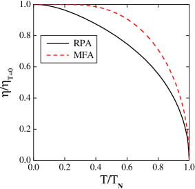
Refer to caption

(a)
Refer to caption (b)

Figure 3: (Color online) The (a) order parameter vs. T/TN𝑇subscript𝑇𝑁T/T_{N} within the RPA method (black solid line) and the MFA (red dashed line), and the (b) spin-wave gaps, in units of J𝐽J, in the spectrum of elementary excitations vs. T/TN𝑇subscript𝑇𝑁T/T_{N} within the RPA method. In both of these figures we have used d/J=0.02𝑑𝐽0.02d/J=0.02, (Γ1Γ3)/J=0.42×103subscriptΓ1subscriptΓ3𝐽0.42superscript103(\Gamma_{1}-\Gamma_{3})/J=0.42\times 10^{-3}, Γ1+Γ3=0subscriptΓ1subscriptΓ30\Gamma_{1}+\Gamma_{3}=0, and Γ2=0subscriptΓ20\Gamma_{2}=0.

Now let us show that in contrast to the MFA approach, where TN=J2Jsubscript𝑇Nsubscript𝐽2𝐽T_{\rm N}=J_{2}\approx J is almost independent of the anisotropy, the Néel temperature within the RPA analytical scheme is very sensitive to model parameters d𝑑d and Γ1Γ3subscriptΓ1subscriptΓ3\Gamma_{1}-\Gamma_{3}.

Refer to caption

(a)
Refer to caption (b)

Figure 4: The (a) T=0𝑇0T=0 energy gaps, in units of J𝐽J, vs. the DM parameter d/J𝑑𝐽d/J, as well as (b) the Néel temperature TNsubscript𝑇𝑁T_{N}, in units of J𝐽J, vs d/J𝑑𝐽d/J. In both of these figures, (Γ1Γ3)/J=0.42×103subscriptΓ1subscriptΓ3𝐽0.42superscript103(\Gamma_{1}-\Gamma_{3})/J=0.42\times 10^{-3}, Γ1+Γ3=0subscriptΓ1subscriptΓ30\Gamma_{1}+\Gamma_{3}=0, and Γ2=0subscriptΓ20\Gamma_{2}=0.

Figure 4 shows the zero-temperature energy gaps and the Néel temperature as functions of the DM antisymmetric exchange interaction d/J𝑑𝐽d/J within the RPA method. As one can see, the energy gap ε1subscript𝜀1\varepsilon_{1} is almost independent of the d/J𝑑𝐽d/J, while ε2subscript𝜀2\varepsilon_{2} depends almost linearly on the DM interaction d/J𝑑𝐽d/J, and in fact goes to the zero in the limit d/J0𝑑𝐽0d/J\to 0. As a result, when d/J=0𝑑𝐽0d/J=0 the Goldstone mode appears in the spin-wave spectrum and thermal fluctuations destroy the long-range ordering for any T>0𝑇0T>0. Consequently, the Néel temperature drops to zero in case of d=0𝑑0d=0.

In the next two figures we present the dependencies on the model parameter (Γ1Γ3)/JsubscriptΓ1subscriptΓ3𝐽(\Gamma_{1}-\Gamma_{3})/J. Now, the energy gap ε2subscript𝜀2\varepsilon_{2} is independent of the parameters of symmetric anisotropy ΓΓ\overleftrightarrow{\Gamma} and thus determined by the DM interaction d/J𝑑𝐽d/J alone, while the gap ε1subscript𝜀1\varepsilon_{1} varies strongly with (Γ1Γ3)/JsubscriptΓ1subscriptΓ3𝐽(\Gamma_{1}-\Gamma_{3})/J.

Refer to caption

(a)
Refer to caption (b)

Figure 5: The (a) energy gaps, in units of J𝐽J, vs. (Γ1Γ3)/JsubscriptΓ1subscriptΓ3𝐽(\Gamma_{1}-\Gamma_{3})/J, and (b) the Néel temperature, in units of J𝐽J, as function of (Γ1Γ3)/JsubscriptΓ1subscriptΓ3𝐽(\Gamma_{1}-\Gamma_{3})/J.

As in the above case, in the limit of Γ1Γ30subscriptΓ1subscriptΓ30\Gamma_{1}-\Gamma_{3}\to 0 the mode ε2subscript𝜀2\varepsilon_{2} in the spectrum becomes gapless and, therefore, the transition temperature to the long-range ordered state would be suppressed to zero.

One can understand the above results for the zone-centre excitation spectrum immediately from the the expressions Eq. (138) in the limit of small anisotropy. Our numerical results, shown in the previous figures, demonstrate that these expressions are valid over a large range of parameter values.

V.2 Parameters regimes

We now summarize our numerical results with regards to the dependence of various thermodynamic quantities on the material parameters appearing in the Hamiltonian.

Firstly, we find that the Néel temperature is almost independent of the (Γ1+Γ3)/JsubscriptΓ1subscriptΓ3𝐽(\Gamma_{1}+\Gamma_{3})/J within the reasonable range of the model parameters (see below).

Refer to caption

(a)
Refer to caption (b)

Figure 6: (Color online) The (a) order parameter vs. T/J𝑇𝐽T/J for the different values of Γ2/JsubscriptΓ2𝐽\Gamma_{2}/J and (Γ1+Γ3)/JsubscriptΓ1subscriptΓ3𝐽(\Gamma_{1}+\Gamma_{3})/J, and (b) the susceptibility, in units of 1/J1𝐽1/J, vs. T/J𝑇𝐽T/J for the different values of Γ2subscriptΓ2\Gamma_{2} and Γ1+Γ3subscriptΓ1subscriptΓ3\Gamma_{1}+\Gamma_{3} discussed in the test. In these plots we have fixed d/J=0.02𝑑𝐽0.02d/J=0.02, and ΔΓ/J(Γ1Γ3)/J=0.42×103ΔΓ𝐽subscriptΓ1subscriptΓ3𝐽0.42superscript103\Delta\Gamma/J\equiv(\Gamma_{1}-\Gamma_{3})/J=0.42\times 10^{-3}).

In fact, in order to argue for the independence of the thermodynamic quantities central to this study on certain material parameters that appear in the Hamiltonian, viz. Γ2subscriptΓ2\Gamma_{2} and Γ1+Γ3subscriptΓ1subscriptΓ3\Gamma_{1}+\Gamma_{3}, in Fig. 6 we show two representative plots for the order parameter and the susceptibility within the RPA scheme for the constant values of the d𝑑d and ΔΓ=Γ1Γ3ΔΓsubscriptΓ1subscriptΓ3\Delta\Gamma=\Gamma_{1}-\Gamma_{3} (again in units of J𝐽J). That is, in each of the plots in Fig. 6 we have simultaneously plotted ten data sets each with the different values of the Γ2subscriptΓ2\Gamma_{2} and Γ1+Γ3subscriptΓ1subscriptΓ3\Gamma_{1}+\Gamma_{3}, where the parameter ratio Γ2subscriptΓ2\Gamma_{2} has been varied from the value 103×ΔΓsuperscript103ΔΓ-10^{3}\times\Delta\Gamma up to the 103×ΔΓsuperscript103ΔΓ10^{3}\times\Delta\Gamma, and Γ1+Γ3subscriptΓ1subscriptΓ3\Gamma_{1}+\Gamma_{3} from the value 102×ΔΓsuperscript102ΔΓ-10^{2}\times\Delta\Gamma to the 102×ΔΓsuperscript102ΔΓ10^{2}\times\Delta\Gamma (all in units of J𝐽J). As one can see, even for such a large range of the parameters, one can hardly see the difference of the absolute values of the Néel temperature, order parameter and susceptibility.

Thus, to study the magnetic properties of the system we can use only the DM interaction d𝑑d and the combination Γ1Γ3subscriptΓ1subscriptΓ3\Gamma_{1}-\Gamma_{3} of the symmetric tensor components as two independent parameters, and so we conclude (similar to othersgozar04 ; Peters ) that the system can be studied using Γ2=0subscriptΓ20\Gamma_{2}=0 and Γ1+Γ3=0subscriptΓ1subscriptΓ30\Gamma_{1}+\Gamma_{3}=0.

In various limits, it can be shown that this result follows from the above presented analytical work. The non-diagonal term Γ2subscriptΓ2\Gamma_{2} of the symmetry anisotropy tensor is involved in all expression through the combination in the J4subscript𝐽4J_{4} (Eq. (42)). For the reasonable anisotropy parameters (that is Γ<dJΓ𝑑much-less-than𝐽\Gamma<d\ll J) the spins are canted by a very small angle θd/Jsimilar-to𝜃𝑑𝐽\theta\sim d/J, and as a result we can neglect the term Γ2sinθdΓ2/Jsimilar-tosubscriptΓ2𝜃𝑑subscriptΓ2𝐽\Gamma_{2}\sin\theta\sim d\Gamma_{2}/J with respect to d𝑑d, and hence we can ignore the quantity Γ2subscriptΓ2\Gamma_{2} in all our formulae. Similarly, Γ1+Γ3subscriptΓ1subscriptΓ3\Gamma_{1}+\Gamma_{3} is involved in the formulae through the combination in the J2subscript𝐽2J_{2}, J3subscript𝐽3J_{3}, and canted angle θ𝜃\theta, where it appeared only as the combination J+12(Γ1+Γ3)𝐽12subscriptΓ1subscriptΓ3J+\frac{1}{2}(\Gamma_{1}+\Gamma_{3}). Thus, the parameter Γ1+Γ3subscriptΓ1subscriptΓ3\Gamma_{1}+\Gamma_{3} can be ignored with respect to the superexchange interaction J𝐽J (see Eq. (42)).

Therefore, one can assert that the model Hamiltonian of Eq. (1) leads to the same results as, for instance, the model described by the spin Hamiltonian

H=i,j[J𝐒i𝐒jΔΓSizSjz+𝐃ij(𝐒i×𝐒j)],𝐻subscript𝑖𝑗delimited-[]𝐽subscript𝐒𝑖subscript𝐒𝑗ΔΓsubscriptsuperscript𝑆𝑧𝑖subscriptsuperscript𝑆𝑧𝑗subscript𝐃𝑖𝑗subscript𝐒𝑖subscript𝐒𝑗H=\sum_{\langle i,j\rangle}[J{\bf S}_{i}\cdot{\bf S}_{j}-\Delta\Gamma S^{z}_{i}S^{z}_{j}+{\bf D}_{ij}({\bf S}_{i}\times{\bf S}_{j})], (143)

where we define ΔΓΓ1Γ3ΔΓsubscriptΓ1subscriptΓ3\Delta\Gamma\equiv\Gamma_{1}-\Gamma_{3}.

V.3 Susceptibility

Now let us consider the main focus of our paper, that being the behaviour of the different components of static uniform magnetic susceptibility as a function of temperature. Our results for χxsuperscript𝜒𝑥\chi^{x}, for the parameters discussed in the previous subsections, are shown in Fig. 7 (recall our earlier result that the MFA and SW theories predict the same T𝑇T-independent value for this quantity). The x𝑥x component of susceptibility below the Néel temperature is the temperature independent and is equal to 1/(8J)absent18𝐽\approx 1/(8J) within the MFA (Eq. (79)), the RPA scheme (Eq. (116)), or spin-wave theory (Eq. (119)). However, above the ordering temperature, the RPA and MFA yield different results, with a weak T𝑇T-dependence within the RPA, while a strong Curie-like falloff is found within the MFA.

Refer to caption
Figure 7: (Color online) The susceptibility χxsuperscript𝜒𝑥\chi^{x}, in units of 1/J1𝐽1/J, within the RPA (black solid line) and MFA (red dashed line), for the parameters values d/J=0.02𝑑𝐽0.02d/J=0.02 and ΔΓ/J=0.42×103ΔΓ𝐽0.42superscript103\Delta\Gamma/J=0.42\times 10^{-3}. Below TNsubscript𝑇𝑁T_{N} these theories both predict the same constant value that is independent of temperature.

As we will discuss in a future publication, this behaviour changes if one includes 4-spin ring exchange, or goes beyond the Tyablikov RPA decoupling scheme that we employ in this paper. This is important since the experimental data of Lavrov et al.,Ando shows a small nonzero slope of χxsuperscript𝜒𝑥\chi^{x} vs. T𝑇T. Indeed, a successful comparison with the small slope seen below TNsubscript𝑇𝑁T_{N} in experimental dataAndo necessarily requires that we go beyond the treatment of spin-wave interactions and/or Hamiltonian that are included in this paper. We emphasize that the necessity of going beyond the Tyablikov RPA decoupling to obtain this slope is a manifestation of the presence of strong quantum fluctuations, a theme that will be repeated in our discussion in this and the next section of this paper.

Our results for the y𝑦y component of the susceptibility, χysuperscript𝜒𝑦\chi^{y}, are shown in Fig. 8.

Refer to caption

(a)
Refer to caption (b)

Figure 8: (Color online) The (a) susceptibility χysuperscript𝜒𝑦\chi^{y} within the RPA (black solid line) and MFA (red dashed line), and (b) a comparison of the RPA (black solid line) and spin-wave (SW) (blue dotted line) results below TNsubscript𝑇𝑁T_{N}. As in previous figures, we are using d/J=0.02𝑑𝐽0.02d/J=0.02 and ΔΓ/J=0.42×103ΔΓ𝐽0.42superscript103\Delta\Gamma/J=0.42\times 10^{-3}.

These plots show that below the ordering temperature the RPA scheme leads to the good agreement with the MFA scheme near the TNsubscript𝑇𝑁T_{N} (0.8TN<T<TN0.8subscript𝑇𝑁𝑇subscript𝑇𝑁0.8T_{N}<T<T_{N}), and good agreement with the SW theory at low-T𝑇T (that is, for T<TN/2𝑇subscript𝑇𝑁2T<T_{N}/2). Above the Néel temperature, the RPA and MFA theories lead to very different results. The MFA method gives an abrupt decrease of χysuperscript𝜒𝑦\chi^{y} to a value that is close to that of the purely transverse component χx1/(8J)superscript𝜒𝑥18𝐽\chi^{x}\approx 1/(8J) (see inset of this figure), while the RPA leads to a much more gradual decrease of the value of χysuperscript𝜒𝑦\chi^{y} with the temperature.

The z𝑧z component of the susceptibility, χzsuperscript𝜒𝑧\chi^{z}, is shown in Fig. 9.

Refer to caption

(a)
Refer to caption (b)

Figure 9: (Color online) The susceptibility χzsuperscript𝜒𝑧\chi^{z} within (a) the RPA (black solid line) and MFA (red dashed line), as well as (b) a comparison of χzsuperscript𝜒𝑧\chi^{z} below the ordering temperature within the RPA (black solid line) and spin-wave (SW) (blue dotted line) theory. As in previous plots, we have used d/J=0.02𝑑𝐽0.02d/J=0.02 and ΔΓ/J=0.42×103ΔΓ𝐽0.42superscript103\Delta\Gamma/J=0.42\times 10^{-3}.

We find that at low T𝑇T, as was also found for χysuperscript𝜒𝑦\chi^{y}, the RPA is in the the good agreement with spin-wave predictions. Near the transition temperature, the RPA method leads to the qualitatively different behaviour of the z𝑧z component of susceptibility with respect to both the MFA and spin-wave formalisms.

The differences between the MFA vs. RPA data shown above can be understood using the following reasoning. Firstly, consider below the Néel temperature. The canted moments which develop are confined to lie in the yz𝑦𝑧y-z plane; as well, they are ferromagnetically ordered in the z𝑧z-direction (recall that we are studying a single CuO2 plane). Then, one can see that within the MFA the weak FM produces a divergence of the z𝑧z-component of the susceptibility only in a very narrow temperature region close to the Néel point. Since the MFA does not account for near-neighbour correlations between the spins, away from the immediate vicinity of TNsubscript𝑇𝑁T_{N} the weak FM is ignored and χzsuperscript𝜒𝑧\chi^{z} behaves like a T𝑇T-independent transverse susceptibility (that is, transverse to the ordered AF moment). In contrast to this, the z𝑧z-component of the susceptibility calculated within the RPA has a strong temperature dependence and shows that the effects of the quantum fluctuations are important in a wide region below the Néel temperature. The other component which shows some differences between the MFA and RPA below the transition is χysuperscript𝜒𝑦\chi^{y}, and for this component it is seen that since the MFA does not include the reduction of the staggered moment (which is in this direction) due to quantum fluctuations at low temperatures, linear spin-wave theory, and not the MFA, agrees with the RPA for low temperatures.

Further, above the Néel temperature the differences can be understood as follows. In a MFA (that is TNMFAJsuperscriptsubscript𝑇𝑁𝑀𝐹𝐴𝐽T_{N}^{MFA}\approx J), both components of the susceptibility χysuperscript𝜒𝑦\chi^{y} and χzsuperscript𝜒𝑧\chi^{z} are rapidly changing functions in the immediate vicinity of TNsubscript𝑇𝑁T_{N} (δT/TN0.005similar-to𝛿𝑇subscript𝑇𝑁0.005\delta T/T_{N}\sim 0.005), and then have the same behaviour as the χxsuperscript𝜒𝑥\chi^{x} term further above the transition. This MFA behaviour is in no way similar to that found in the RPA. That is, our results are an example of the pronounced effects of short-range correlations and quantum fluctuations. The RPA scheme gives a much lower value of the Néel temperature than MFA does (TN0.3Jsimilar-tosubscript𝑇N0.3𝐽T_{\rm N}\sim 0.3J), but in a broad T𝑇T region above the Néel point strong short-range correlations exist, and the RPA includes the manner in which these fluctuations strongly modify the susceptibility. Similar reasoning explains the differences in χxsuperscript𝜒𝑥\chi^{x} between the MFA and RPA.

Refer to caption

(a)
Refer to caption (b)

Figure 10: (Color online) All 3 components of the susceptibility within (a) the MFA, and (b) within the RPA, for d/J=0.02𝑑𝐽0.02d/J=0.02 and ΔΓ/J=0.42×103ΔΓ𝐽0.42superscript103\Delta\Gamma/J=0.42\times 10^{-3}.
Refer to caption

(a)
Refer to caption (b)

Figure 11: (Color online) All 3 components of the susceptibility within (a) the MFA, and (b) within the RPA, for d/J=0.041𝑑𝐽0.041d/J=0.041 and ΔΓ/J=0.42×103ΔΓ𝐽0.42superscript103\Delta\Gamma/J=0.42\times 10^{-3}.
Refer to caption

(a)
Refer to caption (b)

Figure 12: (Color online) All 3 components of the susceptibility within (a) the MFA, and (b) within the RPA, for d/J=0.058𝑑𝐽0.058d/J=0.058 and ΔΓ/J=0.42×103ΔΓ𝐽0.42superscript103\Delta\Gamma/J=0.42\times 10^{-3}.

For completeness, in Figs. 10,11,12 we present all components of the susceptibility together, within both the MFA and the RPA, contrasting different values of the physical parameters describing the DM interaction. To be specific, in Fig. 10 we show the situation when ε1>ε2subscript𝜀1subscript𝜀2\varepsilon_{1}>\varepsilon_{2} with the ratio (ε1/ε2)24.2superscriptsubscript𝜀1subscript𝜀224.2(\varepsilon_{1}/\varepsilon_{2})^{2}\approx 4.2 at zero temperature. As a result, we obtain that for T=0𝑇0T=0 χy<χx,χzsuperscript𝜒𝑦superscript𝜒𝑥superscript𝜒𝑧\chi^{y}<\chi^{x},\chi^{z} with the same ratio between the x,z𝑥𝑧x,z and y𝑦y components of susceptibility χx,z/χy4.2superscript𝜒𝑥𝑧superscript𝜒𝑦4.2\chi^{x,z}/\chi^{y}\approx 4.2 (see §IV.4). By increasing the magnitude of the DM parameter d𝑑d, due to the strong dependence of the mode ε2subscript𝜀2\varepsilon_{2} of the d𝑑d (see Fig. 4), we obtain the situation corresponding to ε2=ε1subscript𝜀2subscript𝜀1\varepsilon_{2}=\varepsilon_{1}. Then, as is seen in Fig. 11, both the MFA and RPA schemes result in equal values of the all components of susceptibility at low T𝑇T. A further increasing ofd𝑑d leads to the situation ε2>ε1subscript𝜀2subscript𝜀1\varepsilon_{2}>\varepsilon_{1}, opposite to the one presented in Fig. 10. In Fig. 12 we show the susceptibility in the case of the ratio (ε2/ε1)22.0superscriptsubscript𝜀2subscript𝜀122.0(\varepsilon_{2}/\varepsilon_{1})^{2}\approx 2.0, and at T=0𝑇0T=0 one finds χy>χx,χzsuperscript𝜒𝑦superscript𝜒𝑥superscript𝜒𝑧\chi^{y}>\chi^{x},\chi^{z} and χy/χx,z2.0superscript𝜒𝑦superscript𝜒𝑥𝑧2.0\chi^{y}/\chi^{x,z}\approx 2.0 for T=0𝑇0T=0. (We note that for other sets of d,ΔΓ𝑑ΔΓd,\Delta\Gamma, the behaviour of the components of χ𝜒\chi is determined almost entirely by the ratio of the spin-wave gaps, ε1/ε2=subscript𝜀1subscript𝜀2absent\varepsilon_{1}/\varepsilon_{2}=. These results agree with our analytical predictions (see section IV).)

Then, comparing the z𝑧z-component of the susceptibility within the RPA (Figs. 10(b)-12(b)) we also find that increasing of the anisotropy parameter d𝑑d leads to the broadening T𝑇T regions where (i) the effects of the quantum fluctuations are important T<TN𝑇subscript𝑇𝑁T<T_{N} and (ii) the strong short-range correlations exists T>TN𝑇subscript𝑇𝑁T>T_{N}.

VI Summary and conclusions/discussion

To summarize, we have presented a theoretical investigation of a single CuO2 plane of the undoped La2CuO4 crystal in the low-T𝑇T orthorhombic phase. The Cu spins in the plane were modelled by the 2D spin-1/2 Heisenberg AF with spin-orbit coupling, the latter represented the antisymmetric and symmetric DM anisotropies. We have adopted the Green’s function method within Tyablikov’s RPA decoupling scheme to calculate the magnetic susceptibility of such a model. In order to allow us to accurately model the longitudinal susceptibility within such a level of decoupling of high-order Green’s functions, we have extended Liu’s method Liu for the isotropic Heisenberg model to one that includes a weak canted FM moment in the plane.

We can emphasize several important conclusions from our results. We have found that the anisotropy introduced into the problem by the symmetric and anti-symmetric DM interactions leads to important changes in the behaviour of the magnetic susceptibility near the transition point. By comparing the MFA and RPA results we conclude that the effects of quantum fluctuations and the short-range correlations are very strong in the broad temperature region of near the Néel temperature. Further, we find that since the RPA and SW results are quite different near the Néel temperature, the effects of spin-wave interactions, which are included in an approximate way in the RPA but not the SW theories, are very important in this system. This necessarily leads to the question, would more advanced decoupling schemes, namely improvements on Tyablikov’s decoupling (e.g., see our Eq. (93)), or, possibly, the inclusion of nonlinear effects in the SW theory, lead to qualitatively different results?

Secondly, we have obtained that the weak ferromagnetism in the z𝑧z-direction (caused by the DM interaction) leads to the essential difference between the temperature behaviours of the transverse χxsuperscript𝜒𝑥\chi^{x} and χzsuperscript𝜒𝑧\chi^{z} components of the susceptibility (recall that the AF moments lie in the yz𝑦𝑧y-z plane and are nearly aligned along the y𝑦y axis). We established the correlation between the ratio of the in- and out-of-plane spin-wave modes of the excitation spectrum in the long wavelength limit (𝒌=0𝒌0{\boldsymbol{k}}=0), which is fixed by the ratio between the d𝑑d and Γ1Γ3subscriptΓ1subscriptΓ3\Gamma_{1}-\Gamma_{3} DM parameters, and the behaviour of χx,zsuperscript𝜒𝑥𝑧\chi^{x,z} vs. χysuperscript𝜒𝑦\chi^{y} in the zero temperature limit. This conclusion is independent on the analytical method which we used to calculate the susceptibilities, since all methods agree in the low-T𝑇T regime, and could allow one to make predictions concerning the gaps in the excitation spectrum based on the data for the susceptibility.

Now we comment on the comparison of our results to the experimentally observed anisotropies Ando that motivated this work. We can state that, in addition to the known resultsCoffey2 ; Aharony1 ; Koshibae that DM interaction induces the weak ferromagnetism in the LTP phase and the spin-wave gaps, this interaction is at least in part responsible for the unusual anisotropy in the magnetic susceptibility.Ando We can mention the most significant features observed in the experiment that are in qualitative agreement with the presented in paper theoretical results: (i) the absence of any special behaviour (anomaly) in the transverse component χxsuperscript𝜒𝑥\chi^{x} across the Néel temperature; (ii) the additional increase of the χysuperscript𝜒𝑦\chi^{y} component in the ordered state and its smooth decrease in a broad temperature region in the paramagnetic state; (iii) a significant temperature dependence of the component χzsuperscript𝜒𝑧\chi^{z} in the broad temperature region below and above the transition point.

Now we briefly discuss the experimental data which cannot be explained within the framework of the proposed here theory. Firstly, we have found that the observed ratio between the x𝑥x and y𝑦y components χx<χysuperscript𝜒𝑥superscript𝜒𝑦\chi^{x}<\chi^{y} (in the T=0𝑇0T=0 limit) takes place only if the spin-wave gap with out-of-plane mode is less than the in-plane one εo<εisubscript𝜀osubscript𝜀i\varepsilon_{\rm o}<\varepsilon_{\rm i}. However, older neutron-scattering experimentsKeimer find the opposite ratio: the magnitude for the out-of-plane mode is 5 meV, for the out-of-plane mode 2.3 meV. Recent Raman work confirms one of these values.gozar04 So, other interactions which affect these gaps must be important for an accurate explanation of the susceptibility data. Secondly, our results cannot explain a T𝑇T-independent shift between χx,χysuperscript𝜒𝑥superscript𝜒𝑦\chi^{x},\chi^{y} and χzsuperscript𝜒𝑧\chi^{z} observed in experiments – an explanation of this physics is provided in the experimental paper, namely that one must include a van Vleck contribution which shifts, in a T𝑇T-independent manner, these components of the susceptibility, but we defer our inclusion of this physics until the second paper in this series of theoretical studies.

For further improvements of our theoretical modelling of the La2CuO4 compound, it seems to be important to investigate a 3D model on a body-centered lattice with the weak AF interlayer coupling. It is also possible to extend the 2D model by considering the ring exchange, and the interaction between the next nearest neighbour sites, and we expect that some of these additional physics can be responsible for the correct ratio between the spin-wave gaps with respect to the ratio between χxsuperscript𝜒𝑥\chi^{x} and χysuperscript𝜒𝑦\chi^{y}. In addition, the anisotropic Van Vleck contribution (orbital susceptibility) and gyromagnetic (Landé) factor need to be taken into account. We will present a detailed comparison to these experiments when these other interactions are included in future publications.

Acknowledgements.
We wish to thank Yoichi Ando, Alexander Lavrov and David Johnston for helpful discussions. One of us (RJG) thanks the Aspen Center for Physics, where part of this work was completed. This work was partially supported by the NSERC of Canada and NATO.

References

  • [1] A.J. Millis, H. Monien, and D. Pines. Phys. Rev. B, 42:167, 1990.
  • [2] E. Manousakis. Rev. Mod. Phys., 63:1, 1991.
  • [3] T. Thio, T.R. Thurston, N.W. Preyer, P.J. Picone, M.A. Kastner, H.P. Jenssen, D.R Gabbe, C.Y. Chen, R.J. Birgeneau, and A. Aharony. Phys. Rev. B, 38:905, 1988.
  • [4] M.A. Kastner, R.J. Birgeneau, T.R. Thurston, P.J. Picone, H.P. Jenssen, D.R. Gabbe, M. Sato, K. Fukuda, S. Shamoto, Y. Endoh, K. Yamada, and G. Shirane. Phys. Rev. B, 38:6638, 1988.
  • [5] B. Keimer, R.J. Birgeneau, A. Cassanho, Y. Endoh, M. Greven, M.A. Kastner, and G Shirane. Z. Phys. B, 91:373, 1993.
  • [6] A.N. Lavrov, Y. Ando, S. Komiya, and I. Tsukada. Phys. Rev. Lett., 87:0170071, 2001.
  • [7] I. Dzialoshinski. J. Phys. Chem. Solids, 4:241, 1958.
  • [8] T. Moriya. Phys. Rev., 120:91, 1960.
  • [9] J. Stain. Phys. Rev. B, 53:785, 1996.
  • [10] In this notation the c𝑐c axis points perpendicular to the cuo2 plane.
  • [11] T. Thio and A. Aharony. Phys. Rev. Lett., 73:894, 1994.
  • [12] D. Coffey, T.M. Rice, and F.C. Zhang. Phys. Rev. B, 44:10 112, 1991.
  • [13] L. Shekhtman, O. Ebtin-Wohlman, and A. Aharony. Phys. Rev. Lett., 71:468, 1993.
  • [14] W. Koshibae, Y. Ohta, and S. Maekawa. Phys. Rev. B, 50:3767, 1994.
  • [15] J. Stain, O. Ebtin-Wohlman, and A. Aharony. Phys. Rev. B, 53:775, 1996.
  • [16] S.V. Tyablikov. Ukrain. Mat. Zh, 11:287, 1959.
  • [17] K.H. Lee and S.H. Liu. Phys. Rev., 159:390, 1967.
  • [18] D.P. Arovas and A. Auerbach. Phys. Rev. B, 38:316, 1988.
  • [19] S. Sarker, C. Jayaprakash, H.R. Krishnamurthy, and M. Ma. Phys. Rev. B, 40:5028, 1989.
  • [20] T.N. de Silva, M. Ma, and F.C. Zhang. Phys. Rev. B, 66:104417, 2002.
  • [21] M. Takahashi. Phys. Rev. B, 40:2494, 1989.
  • [22] V.Yu. Irkhin, A.A. Katanin, and M.I. Katsnelson. Phys. Rev. B, 60:1082, 1999.
  • [23] I. Affleck and J.B. Marston. Phys. Rev. B, 37:3774, 1988.
  • [24] A. Sherman and M. Schreiber. Phys. Rev. B, 63:214421, 2001.
  • [25] Yu.A. Izyumov, N.I. Chaschin, and V.Yu. Yushankhai. Phys. Rev. B, 65:214425, 2002.
  • [26] S. Chakravarty, B.I. Halperin, and D.R. Nelson. Phys. Rev. B, 39:2344, 1989.
  • [27] David C. Johnston. Handbook of Magnetic Materials, 1996.
  • [28] N.E. Bonesteel. Phys. Rev. B, 47:11302, 1993.
  • [29] D. Coffey, K.S. Bedell, and S.A. Trugman. Phys. Rev. B, 42:6509, 1990.
  • [30] D. Mermin and X. Wagner. Phys. Rev. Lett., 17:1133, 1966.
  • [31] S.H. Liu. Phys. Rev., 142:267, 1967.
  • [32] A. Gozar, B.S. Dennis, G. Blumberg, S. Komiya, and Y. Ando. Phys. Rev. Lett., 93:027001, 2004.
  • [33] C.J. Peters, R.J. Birgeneau, M.A. Kastner, H. Yoshizawa, Y. Endoh, J. Tranquada, G. Shirane, Y. Hidaka, M. Oda, M. Suzuki, and T. Murakami. Phys. Rev. B, 37:9761, 1988.