Fluctuations and Defects in Lamellar Stacks of Amphiphilic Bilayers

Abstract

We review recent molecular dynamics simulations of thermally activated undulations and defects in the lamellar $L_{\alpha}$ phase of a binary amphiphile-solvent mixture, using an idealized molecular coarse-grained model: Solvent particles are represented by beads, and amphiphiles by bead-and-spring tetramers. We find that our results are in excellent agreement with the predictions of simple mesoscopic theories: An effective interface model for the undulations, and a line tension model for the (pore) defects. We calculate the binding rigidity and the compressibility modulus of the lamellar stack as well as the line tension of the pore rim. Finally, we discuss implications for polymer-membrane systems.

1 Introduction

Amphiphilic molecules, such as lipids, contain hydrophilic (water loving) and hydrophobic (water fearing) parts. In water, they self-assemble spontaneously such that the hydrophobic parts are shielded from the water environment. One of the most prominent structures is the lamellar phase, where the amphiphiles are arranged in stacks of bilayers. Lipid bilayers are of special interest, because they are essential components of biological membranes.

Phenomenologically, membranes are often described as two dimensional surfaces. A stack of nearly planar membranes of average distance $\bar{d}$ can be parametrized by a set of functions $u_{n}({\bf x})$, where ${\bf x}=(x_{1},x_{2})$ are coordinates in the plane and $x_{3}=u_{n}+n\bar{d}$ denotes the position of the $n$th membrane in the direction perpendicular to the plane. The simplest theoretical Ansatz approximates the free energy of such a stack by [1]

$$E_{\mbox{el}}=\sum_{n}\!\!\int_{A}\!\!\mbox{d}^{2}x\left\{\frac{K_{c}}{2}(\Delta u_{n})^{2}+\frac{B}{2}(u_{n+1}\!\!-\!\!u_{n})^{2}\right\}$$ (1)

with the bending rigidity $K_{c}$ and the compressibility $B$. This free energy functional describes thermally activated membrane undulations with a characteristic in-plane correlation length $\xi=(K_{c}/B)^{1/4}$.

Apart from undulations, membrane stacks also contain defects. Among these, the membrane pores are particularly important, because they influence crucially the permeation properties of the membrane. In the simplest phenomenological model for pore formation [2], a pore with the area $a$ and the contour length $c$ has the free energy

$$E_{\mbox{pore}}=E_{0}+\lambda c-\gamma a,$$ (2)

where $\gamma$ is the surface tension of the membrane and $\lambda$ a line tension. In an isotropic membrane stack, the membranes are tensionless with $\gamma=0$.

In the present paper, we describe large scale molecular dynamics simulations of a molecular coarse-grain model which allow to test these simple theoretical concepts. We find that the models models (1) and (2) capture the physics of our membrane stacks very well. The results are then used to discuss a more complex system, i.e., a polymer inserted in a membrane stack.

2 Simulation Model, Method, and Data Analysis

The simulation model was derived from a similar model by Soddemann et al [3]. The “molecules” consist of two types of beads, $H$ or $P$. “Solvent” particles are single $P$ beads, “Amphiphiles” are $H_{2}P_{2}$ tetramers. All beads have the same mass $m$ and diameter $\sigma$ and interact with a repulsive hard core potential. In addition, beads of the same type attract each other. At appropriate parameter values, the amphiphiles self-assemble spontaneously and form a lamellar stack of bilayers.

Our simulations were carried out in the NPT ensemble with a Langevin thermostat. All sides of the simulation box were allowed to fluctuate in order to ensure isotropic pressure. We studied systems containing a total number of 153600 beads, 30720 of which were solvent particles, at pressure $P=2.9k_{B}T/\sigma^{3}$. The total run length was $10^{7}$ MD steps, corresponding to the time span $10^{5}\sqrt{m\sigma^{2}/k_{B}T}$. The initial equilibration time was $10^{6}$ MD steps. Further details can be found in Refs. [4, 5].

To analyze the data, the simulation box was subdivided into columns of diameter $\sim 1.3\sigma$, perpendicular to the membranes. For each configuration and in each column, the local profiles were determined. This allowed to localize the membranes and to identify membrane defects [4, 5].

3 Results

Membrane Structure and Thermal Fluctuations

Figure 1: Total density profiles (top) and partial volume fractions of head, tail and solvent beads. (Head and tail beads refer to $P$ and $H$ beads of amphiphiles).

The local membrane structure can be characterized by the local density and composition profiles. In order to eliminate the smearing effect of the undulations, we calculate the profiles in each column separately and shift it by the local interface position before averaging. The results are shown in Fig. 1. The total density varies very little throughout the system, but the amphiphile and solvent layers are nevertheless well-separated.

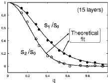
Figure 2: Transmembrane structure factor, fitted to the prediction of the model 1 with one fit parameter $\xi=(K_{c}/B)^{1/4}$.

From the statistics of the interface positions, we can analyze the capillary wave spectrum. Here we show only the transmembrane structure factor between membranes, which we define as $S_{n}(q)=\langle u_{n}({\bf q})^{*}u_{0}({\bf q})\rangle,$ where $u_{n}({\bf q})$ is the two dimensional Fourier transform of $u_{n}({\bf x})$. Within the model (1), we can calculate the quantity $S_{n}(q)$ theoretically and compare the results with the simulation data. The only fit parameter is the parallel correlation length $\xi=(K_{c}/B)^{(1/4)}$. Fig. 2 shows that the theoretical prediction fits the data very well at $\xi=2.34\sigma$.

Similar fits allow to determine the layer distance $\bar{d}=6.38\sigma$, and the Caillé parameter $\eta_{1}=\pi k_{B}T/2\bar{d}^{2}\sqrt{K_{c}B}=0.053$. This gives us all the parameters of the model (1), i.e., $K_{c}=4k_{B}T$ and $B=0.13k_{B}T/\sigma^{4}$.

Pore Defects

The main defects in our system were pores, and only these were studied in detail. The density profiles of the pores (not shown here, see Ref. [5]) show unambiguously that larger pores are hydrophilic, i.e., the amphiphiles at the pore rim rearrange themselves such that the solvent in the pore is shielded from the hydrophobic molecules tails. Since our amphiphiles are very short, the energy penalty on pores is low and the number of pores in the membranes is comparatively large. Nevertheless, we have established in several tests that the pores are essentially uncorrelated. Therefore, pore interactions can be neglected, and we can attempt to interpret our data in terms of the model (2) with $\gamma=0$.

The validity of Eq. 2 was tested in several ways. First, we verified that the pore contour lengths $c$ were distributed according to a Boltzmann distribution. This allowed to extract the value of the line tension, $\lambda=0.7k_{B}T/\sigma$. Next we studied the shape of the pores. Since the membranes have no surface tension, the pores are not circular: At $\gamma=0$, Eq. 2 describes an ensemble of self avoiding ring chains. These should have by the fractal dimension of two-dimensional self-avoiding polymers, characterized by the Flory exponent $\nu_{2}=3/4$. For example, the area $a$ of the pores scales with the contour length like $a\propto c^{3/2}$. Fig. 3 a) shows that the simulation data are compatible with this scaling behavior.

The energy model 2 also has implications for the pore dynamics: The dynamical evolution of the pore contour lengths should correspond to a random walk in a linear potential, $E=E_{0}+\lambda c$. This stochastic model has been solved analytically [6] and we can compare our data with exact results, e.g., for first passage time distributions. As Fig. 3 b) demonstrates, the agreement is again very satisfactory.

Figure 3: Tests of the line tension model (2). Top: Mean area $a$ of pores as a function of contour length $c$. Bottom: Probability that a pore with contour length $c=10$ reaches the contour $c=8$ for the first time at the time $t$, compared with the theoretical prediction for a random walk in a linear potential (RW-LP model [6]).

4 Outlook: Polymer-Membrane Systems

The success of the phenomenological description (1) and (2) motivates its application to more complex situations. As an example, we shall now discuss the effect of inserting a hydrophilic polymer in our system. Two possible scenarios are illustrated in Fig. 4 (left): Either the polymer stays squeezed between two membranes and deforms them locally, or it spans between layers, creating one or several holes.

We have performed simulations of a membrane stack containing a polymer with $100$ $H$-beads [7]. In free $H$-solution, the polymer exhibits self-avoiding walk statistics with the Kuhn length $a=0.4\sigma$. A configuration in a membrane stack is shown in Fig. 4 (right). The polymer induces a hole in one of the adjacent membranes and collapses into a globule which spreads between two layers.

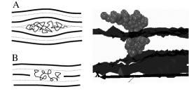
Figure 4: Left: Possible ways of incorporating a polymer in a membrane stack: A – Squeezed between two membranes; B – Spanning several layers and creating a hole. Right: Configuration snapshot of a polymer of length $N=100$ in the membrane stack. The surfaces show the mid-planes of two membranes close to the polymer.

The situation can be analyzed using scaling arguments. The entropy penalty for confining a polymer of length $N$ into a disk of width $R_{\perp}$ and diameter $R_{\parallel}$ is [8, 7]

$$E_{\mbox{c}} \sim N({a}/{R_{\perp}})^{5/3}+N^{3}{a^{5}}/({R_{\perp}R_{\parallel}^{4}})\quad R_{\parallel}>R_{\parallel}^{c}$$ (3)

$$E_{\mbox{c}} \sim N^{9/4}({a^{3}}/{R_{\perp}R_{\parallel}^{2}})^{5/4}\qquad\qquad\quad R_{\parallel}<R_{\parallel}^{c}$$ (4)

with $R_{\parallel}^{c}\sim N^{1/2}R_{\perp}^{1/6}a^{5/6}$. Eq. 3 corresponds to a 2D compressed (pancake) regime, where the main entropic penalty comes from the confinement in the $R_{\perp}$ direction (first term), and the polymer behaves like a slightly compressed 2D self avoiding walk in the $R_{\parallel}$ direction (second term). Eq. 4 describes a 3D compressed regime.

In the scenario A of Fig. 4, $E_{\mbox{p}}$ has to be balanced with the elastic energy $E_{\mbox{el}}$ of the membrane stack. From Eq. 1, we can derive [7] $E_{\mbox{el}}\sim\pi K_{c}(R_{\parallel}\>\delta)^{2}/\xi^{4}$, where $\delta$ is the deformation of the membranes closest to the polymer. In the scenario B, the elastic energy can be neglected, and the polymer compression energy has to be balanced with the energy of pore formation, $E_{\mbox{pore}}\sim 2\pi\lambda R_{\parallel}$.

Details of the calculation will be given elsewhere [7]. Here we merely sketch some of the results: Short chains remain squeezed between membranes (scenario A) and assume a 2D compressed (pancake) structure. In this regime, the total energy scales linearly with $N$. Long chains collapse into a 3D compressed globule, which creates one pore and spans exactly two layers (scenario B). Here, the total energy scales with $N^{9/14}$. In stacks with low compressibility (large $B\bar{d}^{4}$), 2D compressed states spanning two or several layers may appear at intermediate chain lengths.

This qualitatively explains the observation in the simulation: The polymer is in the long chain regime, collapses into the 3D compressed state and spreads between two layers. The agreement is not yet quantitative. According to the scaling theory, the transition to the long-chain regime is expected at the chain length $N_{c}\sim\lambda^{2}a^{-5/3}\bar{d}^{11/3}$, which corresponds to $N\sim 2000$ with our parameter values. Our chain is much shorter. The discrepancy can presumably be explained by the unknown prefactor in the scaling law for $N_{c}$.

To conclude, the phenomenological models (1) and (2) are useful to analyze not only pure membrane stacks, but also polymer-membrane systems. It is remarkable that both the scaling theory and the simulations predict that long (non-adsorbing) hydrophilic polymers enforce pore formation in the membranes.

We thank Ralf Eichhorn, Ralf Everaers, Kurt Kremer, Peter Reimann, Thomas Soddeman, and Hong-Xia Guo for stimulating discussions. The simulations were carried out at the computer centers of the Max-Planck society (Garching) and the Commissariat à l’Energie Atomique (Grenoble).

References

- [1] N. Lei, C. R. Safinya, R. F. Bruinsma, Discrete harmonic model for stacked membranes: theory and experiment, J. Phys. II 5 (8) (1995) 1155.
- [2] J. D. Lister, Stability of lipid bilayers and red blood cell membranes, Physics Letters 53A (1975) 193.
- [3] T. Soddemann, B. Dünweg, K. Kremer, A generic computer model for amphiphilic systems, Eur. Phys. J. E 6 (5) (2001) 409.
- [4] C. Loison, M. Mareschal, K. Kremer, F. Schmid, Thermal fluctuations in a lamellar phase of a binary amphiphile-solvent mixture: A molecular-dynamics study, J. Chem. Phys. 119 (24) (2003) 13138.
- [5] C. Loison, M. Mareschal, F. Schmid, Pores in bilayer membranes of amphiphilic molecules: Coarse-grained molecular dynamics simulations compared with simple mesoscopic models, J. Chem. Phys. 121 (4) (2004) 1890.
- [6] M. Khanta, V. Balakrishnan, First passage time distribution for finite one-dimensional random walks, Pramana 21 (2) (1983) 111.
- [7] C. Loison et al, in preparation.
- [8] M. Daoud, P.-G. de Gennes, Statistics of macromolecular solutions trapped in small pores, J. Phys. II 38 (1) (1977) 85.