Sandpile model on a quenched substrate generated by kinetic self-avoiding trails

Abstract

Kinetic self-avoiding trails are introduced and used to generate a substrate of randomly quenched flow vectors. Sandpile model is studied on such a substrate with asymmetric toppling matrices where the precise balance between the net outflow of grains from a toppling site and the total inflow of grains to the same site when all its neighbors topple once is maintained at all sites. Within numerical accuracy this model behaves in the same way as the multiscaling BTW model.

Accurate determination of the critical exponents and thereby precise distinction of critical behaviors among the different universality classes are always regarded as very important tasks in the field of critical phenomena since this study helps in understanding as well as identification of the crucial factors that determine the critical behaviors. This problem however is still open in the phenomenon of Self-organized criticality (SOC) in spite of extensive research over last several years. More precisely, in the sandpile model of SOC the question if the two very important models namely the deterministic model by Bak, Tang and Wiesenfeld (BTW) Bak and the stochastic Manna sandpile Manna belong to the same universality class or not has not been fully settled yet. A number of works claimed that they belong to the same universality class Pietronero ; Vespignani ; Chessa , where as a number of other papers Ben-Hur ; Lubeck ; Biham2 argue in favor of their universality classes being different. However, what was very much lacking till recently is the precise identification of a key factor which may control the two behaviors.

In SOC Bakbook ; Dhar1 a system evolves to a critical state by a self-organizing dynamics under a constant, slow external drive in the absence of a fine tuning parameter. The signature of the critical state is the spontaneous emergence of long ranged spatio-temporal correlations in the stationary state. The concept of SOC, has been used to explain non-linear transport processes of physical entities like mass, energy, stress etc. in phenomena like sandpiles Bak ; Manna , earthquakes Sornette , forest fires Drossel , biological evolution Baksneppen etc. The transport manifests itself as intermittent activity bursts called avalanches. Sandpile models are the prototype models of SOC. In spite of extensive efforts BTW model resisted to follow the finite size scaling (FSS) ansatz and has been shown recently to obey a multiscaling behavior Stella1 ; Stella2 . On the other hand scaling behavior in the Manna stochastic sandpile Manna is observed to be well behaved Stella2 ; Lubeck ; Biham2 .

A deterministic sandpile model can be defined suitably on an arbitrary graph by an integer toppling matrix (TM) $\Delta$ Dhar1 . For example, on a square lattice of linear size $L$, the number of sand grains at site $i$ is denoted by $h_{i}$. Sand grains are added to the system one by one as: $h_{i}\to h_{i}+1$. A threshold value $H_{i}$ of the number of grains is associated with every site. A toppling occurs at the site $i$ when $h_{i}>H_{i}$. After the toppling the system is updated using the TM of size $L^{2}\times L^{2}$ as: $h_{j}\to h_{j}-\Delta_{ij}$ for $j=1$ to $L^{2}$, where $\Delta_{ii}=H_{i}>0$ for all $i$ and $\Delta_{ij}\leq 0$ for all $i\neq j$. Therefore during a toppling at the site $i$, the number of grains at this site is reduced by $\Delta_{ii}$ where as $-\Delta_{ij}$ number of grains flow out to all sites $j$, $j$ = 1 to $L^{2}$. A toppling at one site may make some of its neighboring sites unstable, which may trigger topplings at further neighborhood, thus creating an avalanche of topplings in a cascade. The BTW model is a special case of deterministic sandpiles where the TM has a simple structure like $H_{i}=4$ and $\Delta_{ij}=\Delta_{ji}=-1$ for each bond $(ij)$, otherwise zero Dhar1 . In the Manna stochastic sandpile model each grain of the toppling site is transferred to a randomly selected neighboring site implying that the TM has the annealed randomness and the elements of $\Delta$ matrix is constantly updated during the whole course of a given avalanche.

Recently a single sandpile model with quenched random toppling matrices is proposed which captures the crucial features of different sandpile models Rumani . In this model the elements of the TM are quenched random variables, once their values are selected in the beginning, they remain unchanged. The dynamics of the sandpile is followed with this TM and the data for avalanches are averaged over different random realizations of TMs. In this model, there can be two possible situations. In the ‘undirected’ case the TM is symmetric i.e., $\Delta_{ij}=\Delta_{ji}$ where as in the ‘directed’ case the TM is asymmetric i.e., $\Delta_{ij}\neq\Delta_{ji}$ in general. Here, $\Delta_{ij}$ is nonzero only for $i=j$ and for each bond of the lattice. It is argued that the behavior of undirected model is similar to the BTW model where as that of the directed model is similar to the Manna model. The distinction between the two models is made even more precise by defining two quantities like $H_{i}=-\sum_{j\neq i}\Delta_{ij}$ i.e., the total number of grains distributed to the neighbors in a single toppling and $H_{i}^{{}^{\prime}}=-\sum_{j\neq i}\Delta_{ji}$ which is the number of grains received by the site $i$ when its every neighbor $j$ topple for once. It has been suggested that the precise balance at all sites (except at the boundary sites)

$$H_{i}=H_{i}^{{}^{\prime}}$$ (1)

ensures that the model obeys the same multiscaling as in the BTW model. For the directed model this precise balance is absent in general and the model shows FSS with the same exponents as in the Manna sandpile model.

Figure 1: A KSAT loop on the square lattice starting from the encircled site and coming back to the same site after 90 steps.

In this paper we extend the results of this paper Rumani and make the conclusion even more precise. We claim that only the precise balance $H_{i}=H_{i}^{{}^{\prime}}$ or the absence of it determines if a model sandpile would belong to the BTW or Manna universality class, irrespective of the TM being symmetric or asymmetric.

A quenched configuration of random flow vectors which corresponds to an asymmetric TM whose elements satisfy eqn. (1) is generated in the following way. Let the neighbors of the site $i$ be denoted by 1, 2, 3 and 4. We first observe that if one increases the $\Delta$ value of any one of the four outgoing bonds, say $(i3)$ by an amount $\delta$, the bond $(i3)$ becomes asymmetric and it increases $H_{i}$ by the same amount. Similarly if we increase the $\Delta$ value of an arbitrary incoming bond to the site $i$, say $(2i)$ by $\delta$ again, the bond $(2i)$ also becomes asymmetric and $H_{i}^{{}^{\prime}}$ increases by an amount $\delta$. Therefore as a result of both the operations the precise balance of $H_{i}=H_{i}^{{}^{\prime}}$ is strictly maintained. In general a series of such bond asymmetrizations can be done randomly by starting from any arbitrary site $i$, selecting randomly an arbitrary outgoing bond $(ij)$, increasing $\Delta_{ij}$ by $\delta$, going to the site $j$, selecting an arbitrary outgoing bond $(jk)$ $(\neq(ji))$ and increasing $\Delta_{jk}$ also by the same amount $\delta$, then going to the site $k$ and so on. The path obviously cannot visit a bond of the lattice more than once and the final point to stop must be the starting point. Such a path can intersect itself but always one of the outgoing bonds which has not been asymmetrized yet is selected randomly. Since at each site on the path the $\Delta$ values of either a single or a double pair of incoming and outgoing bonds have been increased by the same amount $\delta$ the balance of $H_{i}=H_{i}^{{}^{\prime}}$ is maintained at all sites on the path.

Figure 2: (a) Scaling of KSAT loop length distribution for system sizes $L$ = 513, 1025 and 2049. (b) The mean end-to-end distance of KSATs after $n$ steps grows as $n^{2\nu}$.

A self-avoiding trail is a random walk which does not visit one bond of the lattice more than once Malakis . A random configuration of self-avoiding trail is generated by growing a random walk which terminates when a bond is visited more than once. In contrast a kinetic self-avoiding trail (KSAT) is executed with a little more intelligence. At each site, to make a step, the walker first finds out the subset of bonds which has not been visited yet and then steps randomly along any one of these bonds with equal probability. Such a walk can also terminate only when it visits the origin for the third time (Fig.1). A similar definition of kinetic growth walk or growing self-avoiding walks have been studied in the literature and it is argued that very long such walks behave in the same way as ordinary self-avoiding walks Hemmer .

First we observe that KSATs have very interesting and non-trivial statistics. For example the probability distribution that a KSAT returns to the origin for the first time after $n$ steps has a scaling form like:

$$D(n)\sim L^{-\beta}{\cal G}(n/L^{d_{f}})$$ (2)

where the scaling function ${\cal G}(x)\sim x^{-\gamma}$ as $x\to 0$ such that $\gamma=\beta/d_{f}$ and ${\cal G}(x)\to$ decreases to zero very fast when $x\to 1$. We estimated $d_{f}\approx 1.905$, $\beta\approx 2.237$ which give $\gamma\approx 1.174$ (Fig. 2(a)). The cut-off exponent $d_{f}$ is also recognized as the fractal dimension of the KSATs since the number of steps on the walks whose sizes are of the order of $L$ varies as $L^{d_{f}}$. One can also measure the value of $d_{f}$ directly. The mean square end-to-end distance $\langle R^{2}(n)\rangle$ of the walker from the origin after $n$ steps varies as $n^{2\nu}$, where $\nu=1/d_{f}$. Simulation of walks of lengths up to a million steps on a lattice of size $L$ = 4097 gives $\nu\approx 0.530$ so that $d_{f}\approx 1.886$ (Fig. 2(b)). Therefore we conclude a mean value of $d_{f}\approx 1.895$.

KSATs are therefore used to asymmetrize the TM. We start with a TM whose all elements are initially zero corresponding to a periodic $L\times L$ lattice. The walker starts from an arbitrarily selected site, executes a KSAT which finally stops when it comes back to the origin for the first time. The $\Delta$ values of every outgoing bond visited from each site are then increased by $\delta$ which is selected as a random integer number between 1 and 2. A number of such KSAT loops are then generated one by one starting from arbitrarily selected sites and with randomly selected $\delta$ values. The process stops only when all bonds are asymmetrized at least once. The periodic boundary condition is then lifted. The TM so generated is asymmetric in $\approx$ 92.5 % bonds but maintains the precise balance of $H_{i}=H_{i}^{{}^{\prime}}$ strictly at all sites except on the boundary. The lattice is now ready to study the sandpile model where the threshold height at each site is denoted by $H_{i}$. Such a system has a large fluctuation of threshold heights and their average increases with increasing the system size.

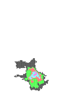
Figure 3: (Color online) Detailed structure of an avalanche, different sites have toppled different number of times: 1(circle), 2(square), 3(triangle up), 4(diamond) and 5(triangle down).

We studied three aspects of the sandpile model on the quenched substrate generated by KSATs which are: (i) the inner structure of the avalanches (ii) the avalanche statistics and the (iii) wave size distributions. We observe very close similarities of our model with BTW model in all three aspects as reported below.

Like any ordinary sandpile model, the dynamics starts from an arbitrary stable distribution of sand heights and then grains are added to the system one by one. The system eventually reaches the stationary state when the average height per site fluctuates around a mean value but does not grow any further. The size of an avalanche is measured by the total number of topplings $s$. In Fig. 3 we show the picture of an avalanche which has no holes. Different sites topple different number of times but the set of sites which toppled same number of times form a connected zone. The avalanche has an inward hierarchical structure, the $n$-th toppling zone is completely surrounded by the $(n-1)$-th toppling zone, with the origin situated within the maximally toppled zone. This is very similar to avalanche structure in the BTW model Grass .

The finite size scaling behavior of the probability distribution Prob($s,L$) of avalanche sizes has the following general form:

$${\rm Prob}(s,L)\sim L^{-\mu}{\cal F}(\frac{s}{L^{D}}),\quad$$ (3)

where the scaling function ${\cal F}(x)\sim x^{-\tau}$ in the limit of $x\to 0$ and ${\cal F}(x)$ approaches zero very fast when $x\to 1$. It is now known that BTW model does not follow this FSS form but has a multiscaling behavior Stella1 ; Stella2 where as the Manna model follows this FSS behavior quite accurately Lubeck .

Figure 4: (a) An attempt for the scaling of the avalanche size distribution for the present model for $L$ = 128, 256 and 512. (b) Comparison of the moment exponents $\sigma(q)$ vs. $q$ and (c) $d\sigma(q)/dq$ vs. $q$ for the present model (solid line) and for the BTW (dotted line) model.

For the present model it is observed that the collapse does not work for a single set of $\mu$ and $D$ and for all values of $s$ and $L$. This is a similar situation as found in the BTW sandpile model and also in the case of undirected quenched model Rumani . For example in Fig. 4(a) we have tried an unsuccessful attempt for a data collapse as: Prob$(s,L)L^{2.4}$ vs. $sL^{-2}$ for $L$ = 128, 256 and 512. Evidently the three curves separate out from one another beyond $s/L^{2}\sim 1$. Even for smaller $s$ values within $1<s<L^{2}$ their slopes differ slightly but systematically as 1.132, 1.135 and 1.144 for $L$ = 128, 256 and 512 respectively, very similar to BTW model behavior.

Further to check that the present model indeed behaves like the multiscaling BTW model the various moments of ${\rm Prob}$ are evaluated Stella1 ; Stella2 ; Lubeck . The $q$-th moment of the avalanche size distribution is defined as $\langle s^{q}\rangle=\Sigma s^{q}{\rm Prob}(s,L)$. Assuming that FSS holds for the whole accessible range of avalanche sizes, it is known that $\langle s^{q}\rangle\sim L^{\sigma(q)}$ where $\sigma(q)=D(q-\tau+1)$ for $q>\tau-1$ and $\sigma(q)=0$ for $0<q<\tau-1$. Estimates of $\sigma(q)$ are obtained from the slopes of the plot of $\log\langle s^{q}(L)\rangle$ with $\log L$ for the three system sizes mentioned above and for 251 equally spaced $q$ values ranging from 0 to 5. In Fig. 4(b) we plot $\sigma(q)$ vs. $q$ for the present model and compare it with a similar plot for the BTW model calculated for the same system sizes, the agreement is found to be very good, within 2%. For both models $\sigma(q)$ shows marked deviation from linearity. To analyze this non-linearity in more detail it is an usual practice to calculate $d\sigma(q)/dq$ which takes the constant value $D$ for large $q$ had the FSS been valid. In contrast, in our present case we see in Fig. 4(c) that $d\sigma(q)/dq$ increases steadily with $q$ for $q>1$ and this plot coincides within the same accuracy with a similar plot for the BTW model.

In a stable configuration if a grain is added to a site $i$ with a height $H_{i}$ it topples and the first wave is the set of all toppled sites while site $i$ is prevented from a second toppling. If $i$ is still unstable after the first wave, the second wave propagates. This process continues until site $i$ becomes stable and the avalanche stops Prie1 ; Prie2 .

Figure 5: This flow chart shows that the precise balance $H_{i}=H_{i}^{{}^{\prime}}$ or absence of it determines the universality classes of different sandpile models.

The autocorrelation function of the wave time series $\{s_{1},s_{2},s_{3},\ldots\}$ of successive waves Stella3 is defined as $C(t,L)=[\langle s_{k+t}s_{k}\rangle_{L}-\langle s_{k}\rangle^{2}_{L}]/[\langle s^{2}_{k}\rangle_{L}-\langle s_{k}\rangle^{2}_{L}]$ where the $\langle..\rangle$ refers quenched disorder averaging. This long range autocorrelation is the consequence of the coherent and uniform spatial structure of each wave. $C(t,L)$ is found to grow steadily with $L$. It scales as $C(t,L)\sim t^{-\tau_{c}}G(t/L^{D_{c}})$ with same exponents as undirected model with $\tau_{c}\approx 0.35$ and $D_{c}\approx 1$. These exponents should be compared to 0.40 and 1.02, respectively, as determined for the BTW model Stella3 .

To summarize, an asymmetric toppling matrix is generated using random kinetic self-avoiding trail loops on the square lattice. The TMs generated in this way guarantees the precise balance between the outflow of grains during a single toppling at a site and the total number of grains flowing into the same site when all its neighbors topple for once. A deterministic sandpile model is studied on such a quenched random lattice and the statistical behavior of its avalanches are compared with that of BTW model in a number of ways, namely, the inner structure of the avalanches, the avalanche statistics and the wave size distributions. Within numerical accuracy excellent agreement is observed in all three categories. We conclude, as displayed in a flow chart in Fig. 5, that it is only the local flow balance or absence of it, irrespective of it being generated from a symmetric or asymmetric TM, determines the universality class of the sandpile model.

References

- (1) P. Bak, C. Tang and K. Wiesenfeld, Phys. Rev. Lett. 59, 381 (1987); P. Bak, C. Tang and K. Wiesenfeld, Phys. Rev. A 38, 364 (1988).
- (2) S.S. Manna, J. Phys. A 24, L363 (1991).
- (3) L. Pietronero, A. Vespignani and S. Zapperi, Phys. Rev. Lett. 72, 1690 (1994).
- (4) A. Vespignani, S. Zapperi and L. Pietronero, Phys. Rev. E 51, 1711 (1995).
- (5) A. Chessa, H. E. Stanley, A. Vespignani and S. Zapperi, Phys. Rev. E 59, 12 (1999).
- (6) A. Ben-Hur and O. Biham, Phys. Rev. E 53, R1317 (1996).
- (7) S. Lübeck, Phys. Rev. E 61, 204 (2000).
- (8) O. Biham, E. Milshtein, and O. Malcai, Phys. Rev. E 63, 061309 (2001).
- (9) P. Bak, How Nature Works: The Science of Self-Organized Criticality, (Copernicus, New York, 1996).
- (10) D. Dhar, Studying Self-Organized Criticality with Exactly Solved Models, arXiv:cond-mat/9909009.
- (11) A. Sornette and D. Sornette, Europhys. Lett. 9, 197 (1989).
- (12) B. Drossel and F. Schwabl, Phys. Rev. Lett. 69, 1629 (1992).
- (13) P. Bak and K. Sneppen, Phys. Rev. Lett. 71, 4083 (1993).
- (14) M. De Menech, A. L. Stella, and C. Tebaldi, Phys. Rev. E 58, 2677 (1998).
- (15) C. Tebaldi, M. De Menech and A. L. Stella, Phys. Rev. Lett. 83, 3952 (1999).
- (16) R. Karmakar, S. S. Manna, and A. L. Stella, cond-mat/0312127.
- (17) A. Malakis, J. Phys. A 8, 1885 (1975); A. Malakis, J. Phys. A 9, 1283 (1976).
- (18) S. Hemmer and P. C. hemmer, J. Chem. Phys. 81, 584 (1984); J. Majid, N. Jan, A. Coniglio and H. E. Stanley, Phys. Rev. Lett. 52, 1257 (1984); J. W. Lyklema and K. Kremer, J. Phys. A, 17, L691 (1984).
- (19) P. Grassberger and S.S. Manna, J. Phys. (Paris) 51, 1077 (1990).
- (20) E. V. Ivashkevich, D. V. Ktitarev, and V. B. Priezzev, Physica A 209, 347 (1994).
- (21) D. V. Ktitarev, S. Lübeck, P. Grassberger, and V. B. Priezzhev, Phys. Rev. E 61, 81 (2000).
- (22) M. De Menech and A. L. Stella, Phys. Rev. E 62, R4528 (2000).