Influence of sequence correlations on the adsorption of random copolymers onto homogeneous planar surfaces

Abstract

Using a reference system approach, we develop an analytical theory for the adsorption of random heteropolymers with exponentially decaying and/or oscillating sequence correlations on planar homogeneous surfaces. We obtain a simple equation for the adsorption-desorption transition line. This result as well as the validity of the reference system approach is tested by a comparison with numerical lattice calculations.

I Introduction

Random heteropolymers (RHPs) currently attract much attention and have been studied intensely in the last two decades. The reason for the growing interest in them is twofold. On the one hand, they can be used to create new polymeric materials, or to modify and improve surface and interface properties. On the other hand, RHPs serve as simple model systems for biologically relevant heterogeneous macromolecules, such as proteins and nucleic acids. Studying the physics of RHPs helps to understand generic properties of these macromolecules and phenomena which play an important role in living organisms, such as protein folding, denaturation/renaturation of DNA, secondary structure formation by RNA, etc.

In the present paper, we consider RHP adsorption on homogeneous and impenetrable (solid) surfaces. This has technological relevance in the context of adhesion (glue) and surface design. Studying RHP adsorption can also be regarded as a (very) first step towards understanding some elementary principles of molecular recognition.

For entirely random RHPs, the problem was investigated theoretically by a number of authors. Joanny Joanny considered the adsorption of polyampholyte chains on a planar solid surface. In the case that the electrostatic interactions are strongly screened and thus short-ranged, he treated the polyampholyte chain as an ideal RHP with no intersegment interactions, and solved the problem using the replica trick and the Hartree approximation. A replica symmetric mean field theory that takes into account intersegment interactions has been developed by Gutman and Chakraborty Gutman1 ; Gutman2 , to describe RHPs interacting with one Gutman2 or two parallel Gutman1 planar surfaces. They analyzed the interfacial structure (as expressed through the density and the order parameter profiles) as well as the adsorption-desorption phase diagram. Stepanow and Chudnovsky Stepanow combined the replica trick with the Greens function technique to study the localization of a RHP onto a homogeneous surface, and suggested a phase diagram for the localization-delocalization transition. The system has been also studied by Monte-Carlo simulations Sumithra ; Moghaddam . Sumithra and Baumgaertner Sumithra have complemented their simulations by a scaling analysis of the conformational and thermodynamic characteristics of the system.

In all of these works the RHPs were taken to be of Bernoullian type, i. e., the monomer sequences had no correlations. Sequence correlations should, of course, affect the adsorption properties of RHPs. van Lent and Scheutjens vanLent have formulated a self-consistent field theory for random copolymers with correlated sequences in the case of annealed disorder, i. e., the copolymer sequences can “adjust” to their local environment. They used it to study the adsorption of random copolymers from solution within a lattice model. Zheligovskaya et al. Zheligovskaya have explored the idea of conformation-dependent sequence design and compared the adsorption properties of AB-copolymers with special “adsorption-tuned” primary structures (adsorption-tuned copolymers, ATC) with those of truly random copolymers. Monte-Carlo simulations revealed that some specific features of the ATC primary structure promote the adsorption of ATC chains, compared to random chains. Chakraborty and coworkers Chakraborty1 ; Chakraborty_review have demonstrated the importance of sequence correlations in a number of studies on recognition between random copolymers and chemically heterogeneous surfaces.

Whereas these studies were mostly numerical, Denesyuk and Erukhimovich Denesyuk have recently presented an approximate analytical solution of a closely related problem, the adsorption of RHPs with sequence correlations on penetrable homogeneous substrates (e. g., interfaces between two selective solvents). Their study is based on a reference system approach originally due to Chen Chen . The sequence correlations were described by a correlator introduced by de Gennes deGennes78 that covers both exponentially decaying and oscillating correlations. Denesyuk an Erukhimovich showed that chains with both types of correlation exhibit a continuous adsorption transition, and constructed the corresponding adsorption-desorption phase diagrams.

In the present paper we extend this work to study the adsorption of RHPs with correlated monomer sequences onto a homogeneous impenetrable planar surface. We use the reference system approach Chen and follow closely the ideas developed in Ref. Denesyuk, . This will allow us to derive an explicit and surprisingly simple analytical expression for the adsorption transition point. To test our prediction, we also performed numerical calculations on the lattice, and compared the results to the premises and the result of the analytical theory.

The rest of the paper is organized as follows: The analytical theory is developed in Sec. II. We begin with defining the model in Sec. II.1, and discuss the theoretical approach in the next three subsections, Sec. II.2, Sec. II.3, and Sec. II.4. The final result is presented in Sec. II.5. Then, we describe the numerical calculations in Sec. III. The numerical calculations are compared to the analytical prediction in Sec. IV. We summarize and conclude in Sec. V.

II Analytical Approach

II.1 Definition of the Model

We consider an ensemble of single heteropolymer Gaussian chains, each consisting of $N$ monomer units, near an impenetrable planar surface. Monomers only interact with the surface, not with each other. The strength and the sign of the monomer-surface interaction varies from monomer to monomer and is characterized by an affinity parameter $\xi$. A particular heteropolymer realization is described by the sequence $\xi(n)$, where $n$ indicates the monomer number ($n=1,2,...,N$). It is, however, convenient to consider $n$ as a continuous rather than a discrete variable. The Hamiltonian of the system can then be represented as follows:

$$\frac{H}{kT}=\frac{3}{2a^{2}}\int_{0}^{N}dn\left(\frac{\partial z}{\partial n}\right)^{2}-\beta\int_{0}^{N}dn\,V(z(n))\,\xi(n),$$ (1)

where the $z$ direction is perpendicular to the surface and we have integrated out the x and y coordinates. Here $\beta=1/kT$ is the Boltzmann factor as usual, $a$ is the Kuhn segment length of the chain, and $V(z)$ gives the shape of the monomer-surface interaction potential ($\int V(z)\>dz=1$), which is taken to be the same for all monomers. More specifically, we use a pseudopotential – a Dirac well shifted by the small but finite distance $z_{0}$ from the impenetrable surface

$$V(z)=\left\{\begin{array}[]{lc}\delta(z-z_{0})&\mbox{if }z>0\\ +\infty&\mbox{if }z<0\end{array}\right.$$ (2)

The parameter $z_{0}>0$ corresponds to the range of the surface potential. It has been introduced mainly for technical reasons, which will become apparent further below. In the end (Sec. II.5), we will take the limit $z_{0}\to 0$.

The sequences $\xi(n)$ are randomly distributed according to a Gaussian probability function

$$P\{\xi(n)\}=\frac{\exp\left[-\frac{1}{2}\int_{0}^{N}dn_{1}\int_{0}^{N}dn_{2}(\xi(n_{1})-\xi_{0})c^{-1}(n_{2}-n_{1})(\xi(n_{2})-\xi_{0})\right]}{\int\mathcal{D}\{\xi(n)\}\exp\left[-\frac{1}{2}\int_{0}^{N}dn_{1}\int_{0}^{N}dn_{2}(\xi(n_{1})-\xi_{0})c^{-1}(n_{2}-n_{1})(\xi(n_{2})-\xi_{0})\right]}.$$ (3)

Here $\xi_{0}=\langle\xi\rangle$ is the mean affinity and $c(n_{1},n_{2})$ describes the sequence correlations. The latter is taken to have the special form suggested by de Gennes deGennes79 ,

$$c(n_{1},n_{2}) \equiv \left\langle(\xi(n_{1})-\xi_{0})(\xi(n_{2})-\xi_{0})\right\rangle$$ (4)

$$= c(|n_{2}-n_{1}|)=\Delta^{2}\mathop{\rm Re}\nolimits\>e^{-\Gamma|n_{2}-n_{1}|},$$

where $\mathop{\rm Re}\nolimits$ denotes the real part of a complex number. This allows us, by proper choice of the parameter $\Gamma$, to cover both exponentially decaying (real $\Gamma$) or oscillating (purely imaginary $\Gamma$) correlations. The expression $\int\mathcal{D}\{\xi(n)\}$ denotes functional integration over all possible sequences (integration in sequence space), and $c^{-1}(n)$ is the inverse function of $c(n)$, defined by $\int\!dn^{\prime}\,c^{-1}(n-n^{\prime})c(n^{\prime})=\delta(n)$.

We will calculate the quenched average over all sequences, i. e., the free energy of the system is the disorder average of the logarithm of the conformational statistical sum, $F=\langle\log Z_{\mbox{\tiny conf}}\rangle_{\xi(n)}$. For infinitely long chains, the adsorption transition in this model is encountered at $F=0$.

II.2 The Reference System Approach

Having defined the model, we now turn to describing the analytical approach. To perform the quenched average we exploit the well-known replica trick

$$\langle\log Z\rangle_{\xi(n)}=\lim_{m\to 0}\langle\frac{Z^{m}-1}{m}\rangle_{\xi(n)}.$$ (5)

This reduces the problem of evaluating the disorder average over a logarithm, $\langle\log Z\rangle$, to the much more feasible task of evaluating the average partition function for a set of $m$ identical heteropolymer chains ($m$ replicas) $\langle Z^{m}\rangle$. Inserting Eqs. (3) - (4) and using properties of the Gaussian distribution, we obtain

$$\begin{split}\langle Z^{m}\rangle_{\xi(n)}=&\int\prod_{\alpha=1}^{m}\mathcal{D}\{z_{\alpha}(n)\}\exp\left[-\frac{3}{2a^{2}}\sum_{\alpha=1}^{m}\int_{0}^{N}dn\left(\frac{\partial z_{\alpha}}{\partial n}\right)^{2}+\beta\xi_{0}\int_{0}^{N}dn\sum_{\alpha=1}^{m}V(z_{\alpha}(n))\right]\\ &\times\exp\left[\frac{\beta^{2}}{2}\int_{0}^{N}dn_{1}\int_{0}^{N}dn_{2}\sum_{\alpha=1}^{m}V(z_{\alpha}(n_{1}))\sum_{\gamma=1}^{m}V(z_{\gamma}(n_{2}))c(n_{2}-n_{1})\right],\end{split}$$ (6)

where $\alpha$ is the replica index and $\int\mathcal{D}\{z(n)\}$ denotes the integration over all possible trajectories $z(n)$ of the chain.

One can easily see that the problematic term in this expression is the last factor which couples different replicas. To simplify this term we introduce a reference homopolymer system Chen whose conformational properties are reasonably close to those of the original heteropolymer. It is natural to choose as reference system a single homopolymer chain with uniform monomer affinity $\xi_{0}+v_{0}$, which is exposed to a surface potential $V(z)$ of the same shape (2) as the original RHP. The parameter $v_{0}$ is a fit parameter which can be adjusted such that the reference system is as close as possible to the original system. It is nonzero and positive, because the effective surface affinity of heteropolymers is generally larger than that of homopolymers with the same charge. For example, even globally neutral random heteropolymers with $\xi_{0}=0$ can adsorb onto a surface, whereas neutral homopolymers obviously remain desorbed.

The Hamiltonian of the reference system has the following form:

$$\frac{H_{0}}{kT}=\frac{3}{2a^{2}}\int_{0}^{N}dn\left(\frac{\partial z}{\partial n}\right)^{2}-\beta(\xi_{0}+v_{0})\int_{0}^{N}\,dn\,V(z(n))$$ (7)

The difference between the free energies of the original and the reference system is given by

$$-\beta(F-F_{0})=\lim_{m\to 0}\frac{Z^{m}-Z_{0}^{m}}{m}$$ (8)

where $Z_{0}^{m}$ is the partition function of the $m$ times replicated reference system:

$$Z_{0}^{m}=\int\prod_{\alpha=1}^{m}\mathcal{D}\{z_{\alpha}(n)\}\exp\left[-\frac{3}{2a^{2}}\sum_{\alpha=1}^{m}\int_{0}^{N}dn\left(\frac{\partial z_{\alpha}}{\partial n}\right)^{2}+\beta(\xi_{0}+v_{0})\int_{0}^{N}dn\,\sum_{\alpha=1}^{m}\ V(z_{\alpha}(n))\right]$$ (9)

Thus one has

$$\begin{split}Z^{m}-Z_{0}^{m}=&\int\prod_{\alpha=1}^{m}\mathcal{D}\{z_{\alpha}(n)\}\times\exp\left[-\frac{3}{2a^{2}}\sum_{\alpha=1}^{m}\int_{0}^{N}dn\left(\frac{\partial z_{\alpha}}{\partial n}\right)^{2}+\beta(\xi_{0}+v_{0})\int_{0}^{N}dn\,\sum_{\alpha=1}^{m}\ V(z_{\alpha}(n))\right]\\ \times&\left\{\exp\left[\frac{\beta^{2}}{2}\int_{0}^{N}dn_{1}\int_{0}^{N}dn_{2}\sum_{\alpha=1}^{m}V(z_{\alpha}(n_{1}))\sum_{\gamma=1}^{m}V(z_{\gamma}(n_{2}))c(n_{2}-n_{1})-\beta v_{0}\int_{0}^{N}dn\,\sum_{\alpha=1}^{m}\ V(z_{\alpha}(n))\right]-1\right\}\end{split}$$ (10)

The first exponential in this expression corresponds to the product of the $m$ independent propagators ${\cal P}(\xi_{0},v_{0},z_{\alpha}(n))$ for the $m$ chains in the replicated reference system, which give the statistical weight of the particular trajectories $z_{\alpha}(n)$. Since the original and the reference systems are assumed to be close to each other, we expand the exponent in the second term: $e^{A}-1\simeq A$. Here $A$ is the difference between Hamiltonians of replicated original and the reference systems $-\beta(H^{m}-H_{0}^{m})$. This means that we approximate the difference between the free energies of the original and the reference system $\Delta F\equiv F_{0}-F$ by its first cumulant $\Delta F_{1}$. The expansion gives

$$\begin{split}Z^{m}-Z_{0}^{m}\simeq&\int\prod_{\alpha=1}^{m}\Big{[}\mathcal{D}\{z_{\alpha}(n)\}{\cal P}(\xi_{0},v_{0},z_{\alpha}(n))\Big{]}\\ &\times\left[\frac{\beta^{2}}{2}\int_{0}^{N}dn_{1}\int_{0}^{N}dn_{2}\sum_{\alpha=1}^{m}V(z_{\alpha}(n_{1}))\sum_{\gamma=1}^{m}V(z_{\gamma}(n_{2}))c(n_{2}-n_{1})-\beta v_{0}\int_{0}^{N}dn\,\sum_{\alpha=1}^{m}\ V(z_{\alpha}(n))\right].\end{split}$$ (11)

The second integral in Eq. (11) is equal to

$$\begin{split}I_{2}&=\int\prod_{\alpha=1}^{m}\Big{[}\mathcal{D}\{z_{\alpha}(n)\}{\cal P}(\xi_{0},v_{0},z_{\alpha}(n))\Big{]}\\ &\qquad\times\>\beta v_{0}\int_{0}^{N}dn\,\sum_{\alpha=1}^{m}V(z_{\alpha}(n))\\ &=\beta v_{0}Nm\overline{V(z(n))}Z_{0}^{m},\end{split}$$ (12)

where $\overline{\cdots}$ denotes the average with respect to the reference system:

$$\overline{X}=\frac{\int\mathcal{D}\{z(n)\}G(\xi_{0},v_{0},z(n))X(z(n))}{\int\mathcal{D}\{z(n)\}G(\xi_{0},v_{0},z(n))}$$ (13)

Next we consider the first integral

$$\begin{split}I_{1}=&\int\prod_{\alpha=1}^{m}\Big{[}\mathcal{D}\{z_{\alpha}(n)\}{\cal P}(\xi_{0},v_{0},z_{\alpha}(n))\Big{]}\\ &\times\frac{\beta^{2}}{2}\int_{0}^{N}dn_{1}\int_{0}^{N}dn_{2}\sum_{\alpha=1}^{m}V(z_{\alpha}(n_{1}))\\ &\times\sum_{\gamma=1}^{m}V(z_{\gamma}(n_{2}))c(n_{2}-n_{1}).\end{split}$$ (14)

The product of the two sums in Eq. (14) gives

$$\sum_{\alpha=1}^{m}V(z_{\alpha}(n_{1}))\sum_{\gamma=1}^{m}V(z_{\gamma}(n_{2}))$$

$$=\sum_{\alpha=1}^{m}V(z_{\alpha}(n_{1}))V(z_{\alpha}(n_{2}))$$

$$+\sum_{\alpha=1}^{m}\sum_{\gamma=1\atop\gamma\neq\alpha}^{m}V(z_{\alpha}(n_{1}))V(z_{\gamma}(n_{2})),$$

where we have separated contributions from the same and different replicas. This leads to the following result for $I_{1}$:

$$I_{1}=\beta^{2}m\,Z_{0}^{m}\int_{0}^{N}dk\,c(k)\,(N-k)\,$$

$$\Big{\{}(m-1)\overline{V(z_{\alpha}(n))V(z_{\gamma}(n+k))}\Big{|}_{\alpha\neq\gamma}$$

$$+\overline{V(z_{\alpha}(n))V(z_{\alpha}(n+k))}\Big{\}}.$$

Finally, collecting all terms, taking the limit $m\to 0$, dividing by $N\gg 1$, and using $c(k)k/N\gg 1$ for all $k$, we obtain for the first cumulant $\Delta F_{1}$

$$\begin{split}\frac{\beta\Delta F_{1}}{N}=&\,\beta^{2}\int_{0}^{N}dk\,c(k)\,\overline{V(z_{\alpha}(n))V(z_{\alpha}(n+k))}\\ &-\beta^{2}\int_{0}^{N}dk\,c(k)\,\overline{V(z_{\alpha}(n))V(z_{\gamma}(n+k))}\Big{|}_{\alpha\neq\gamma}\\ &-\beta v_{0}\overline{V(z_{\alpha}(n))}.\end{split}$$ (17)

The next step is to find the Greens function of the reference system, which is needed for calculating the averages in Eq. (17).

II.3 The Reference System

As defined above, the reference system is a homopolymer chain with the affinity parameter $w_{0}=\xi_{0}+v_{0}$, which propagates in the half space $z>0$ subject to the potential $V(z)=\delta(z-z_{0})$. The Greens function of the polymer chain in the reference system satisfies the differential equation DoiEdwards ; deGennes_book

$$\frac{\partial G}{\partial N}=\frac{a^{2}}{6}\frac{\partial^{2}G}{\partial z^{2}}+\beta w_{0}\delta(z-z_{0})G(z,z^{\prime};N)$$ (18)

with the initial condition

$$G(z,z^{\prime};0)=\delta(z-z^{\prime})$$ (19)

and the boundary conditions

$$\begin{array}[]{rcl}G(z,z^{\prime};N)|_{z\to\infty}&=&0\\ G(z,z^{\prime};N)|_{z=0}&=&0\end{array}.$$ (20)

Eq. (18) has the structure of a Schrödinger equation and can be solved analogously by a separation of variables. The solution is an expansion in eigenfunctions of the “Hamilton operator”,

$$G(z,z^{\prime};N)=\sum_{i}e^{-\varepsilon_{i}N}\psi_{i}(z)\psi_{i}^{*}(z^{\prime}),$$ (21)

where $\varepsilon_{i}$ and $\psi_{i}(z)$ are eigenvalues and eigenfunctions of the stationary equation

$$\frac{a^{2}}{6}\frac{\partial^{2}\psi}{\partial z^{2}}+\beta w_{0}\delta(z-z_{0})\psi(z)=-\varepsilon\psi(z).$$ (22)

For very long chains ($N\gg 1$), the sum (21) is dominated by the largest term, corresponding to the lowest eigenvalue $(-\varepsilon_{0})$ (ground-state dominance):

$$G(z,z^{\prime};N)\simeq e^{-\varepsilon_{0}N}\psi_{0}(z)\psi_{0}^{*}(z^{\prime}).$$ (23)

The analogous problem of quantum-mechanical particle motion in the potential $V(z)$ has been treated in detail by Aslangul Aslangul . To establish the connection to these calculations, we rewrite the stationary differential equation (22) in the form

$$\psi^{\prime\prime}(z)-k^{2}\psi(z)=-k_{0}\delta(z-z_{0})\psi(z),$$ (24)

where $k$ and $k_{0}$ are given by

$$k^{2}=-\frac{6\varepsilon_{0}}{a^{2}}$$ (25)

and

$$k_{0}=\frac{6\beta w_{0}}{a^{2}}=\frac{6\beta(\xi_{0}+v_{0})}{a^{2}}.$$ (26)

The boundary conditions are: $\psi(z)|_{z=0}=0$ and $\psi(z)|_{z\to\infty}=0$. Eq. (24) has the same form as Eq. (3) in Ref. Aslangul, , except that we have chosen $k_{0}>0$, and we can simply apply the results of Ref. Aslangul, . For the ground state eigenfunction we obtain

$$\psi_{0}(z)=A\left[e^{-k_{b}|z-z_{0}|}-e^{-k_{b}(z+z_{0})}\right]$$ (27)

where $k_{b}$, determining the ground-state energy (25), is the root of the transcendental equation

$$\frac{2k}{1-e^{-2kz_{0}}}=k_{0}$$ (28)

and the normalization constant $A$ is equal to

$$A=\left(\frac{k_{0}/2}{1+(2k_{b}-k_{0})z_{0}}\right)^{1/2}.$$ (29)

Eq. (28) always has the trivial solution $k=0$. A nontrivial solution exists if the slope of the line $y=2k$ is smaller than the slope of the curve $y=k_{0}(1-e^{-2kz_{0}})$ at $z=0$. This condition yields the value of the adsorption transition point.

$$k_{0}^{tr}=\frac{1}{z_{0}}.$$ (30)

The expression for the ground-state Greens function is

$$\begin{split}G(z,z^{\prime};N)=&\>\frac{k_{0}/2}{1+(2k_{b}-k_{0})z_{0}}\left[e^{-k_{b}|z-z_{0}|}-e^{-k_{b}(z+z_{0})}\right]\\ &\times\left[e^{-k_{b}|z^{\prime}-z_{0}|}-e^{-k_{b}(z^{\prime}+z_{0})}\right]\>e^{-\epsilon_{0}N}\end{split}.$$ (31)

Based on these results we can now calculate the averages in (17), using the ground-state dominance approximation (23) for the Greens function.

$$\overline{V(z(n))}$$

$$=\frac{\int_{0}^{N}dl\int_{0}^{\infty}dx\,dy\,dz\,G(x,z;l)\delta(z-z_{0})G(z,y;N-l)}{\int_{0}^{N}dl\int_{0}^{\infty}dx\,dy\,dz\,G(x,z;l)G(z,y;N-l)}$$

$$\simeq\int_{0}^{\infty}dz|\psi_{0}(z)|^{2}\delta(z-z_{0})=|\psi_{0}(z_{0})|^{2}$$

$$=A^{2}\left(1-e^{-2k_{b}z_{0}}\right)^{2}=A^{2}\left(\frac{2k_{b}}{k_{0}}\right)^{2}=\frac{2k_{b}^{2}/k_{0}}{1+(2k_{b}-k_{0})z_{0}}$$

Since different replicas are independent, the second term of Eq. (17) becomes

$$\begin{split}\overline{V(z_{\alpha}(n))V(z_{\gamma}(n+k))}\Big{|}_{\alpha\neq\gamma}&=\overline{V(z_{\alpha}(n))}^{\>2}\\ &\simeq\left[\frac{2k_{b}^{2}/k_{0}}{1+(2k_{b}-k_{0})z_{0}}\right]^{2}\end{split}$$ (33)

Inserting these averages in Eq. (17) and using the explicit expression (4) for the correlation function $c(k)$, we obtain for the first cumulant

$$\begin{split}\frac{\beta\Delta F_{1}}{N}=&\beta^{2}\Delta^{2}\mathop{\rm Re}\nolimits\left\{S(\Gamma)-\frac{1}{\Gamma}\left[\frac{2k_{b}^{2}/k_{0}}{1+(2k_{b}-k_{0})z_{0}}\right]^{2}\right\}\\ &-\beta v_{0}\frac{2k_{b}^{2}/k_{0}}{1+(2k_{b}-k_{0})z_{0}}.\end{split}$$ (34)

Here

$$\begin{split}S(\Gamma)=&\int_{0}^{N}dk\,\exp(-\Gamma k)\overline{V(z(n))V(z(n+k))}\\ \simeq&\int_{0}^{\infty}dk\,\exp(-\Gamma k)\overline{V(z(n))V(z(n+k))}\end{split}$$ (35)

is the Laplace transform of $\overline{V(z(n))V(z(n+k))}\equiv s(k)$ and we have used

$$\int_{0}^{N}dk\,c(k)=\frac{\Delta^{2}}{\Gamma}\left(1-e^{-\Gamma N}\right)\stackrel{{\scriptstyle N\gg 1}}{{\simeq}}\frac{\Delta^{2}}{\Gamma}.$$ (36)

Our next task is to calculate $s(k)$ and $S(p)$. By definition, we have

$$\begin{split}s(k)&=\frac{\int_{0}^{N}\!\!dl\int_{0}^{\infty}dx\,dy\,dz\,dz^{\prime}\,G(x,z;l)\delta(z-z_{0})G(z,z^{\prime};k)V(z^{\prime})G(z^{\prime},y;N-l-k)}{\int_{0}^{N}\!\!dl\int_{0}^{\infty}dx\,dy\,dz\,dz^{\prime}\,G(x,z;l)G(z,z^{\prime};k)G(z^{\prime},y;N-l-k)}\end{split}$$ (37)

We adopt the ground-state dominance approximation for the overall chain and for the side subchains in Eq. (37). This yields for $s(k)$

$$s(k)\simeq e^{k\varepsilon_{0}}\int_{0}^{\infty}dz\,dz^{\prime}\,V(z)\psi_{0}(z)V(z^{\prime})\psi_{0}(z^{\prime})G(z,z^{\prime};k)$$ (38)

and for the Laplace transform

$$S(p)\simeq\int_{0}^{\infty}\!\!\!\!\!dz\,dz^{\prime}\,V(z)\psi_{0}(z)V(z^{\prime})\psi_{0}(z^{\prime})\mathcal{G}(z,z^{\prime};p+|\varepsilon_{0}|)$$ (39)

$$= \int_{0}^{\infty}\!\!\!\!\!\!dz\,dz^{\prime}\,\delta(z\!-\!z_{0})\psi_{0}(z)\delta(z^{\prime}\!-\!z_{0})\psi_{0}(z^{\prime})\mathcal{G}(z,z^{\prime};p+|\varepsilon_{0}|)$$

$$= [\psi_{0}(z_{0})]^{2}\mathcal{G}(z_{0},z_{0};p+|\varepsilon_{0}|)$$

$$= \frac{2k_{b}^{2}/k_{0}}{1+(2k_{b}-k_{0})z_{0}}\mathcal{G}(z_{0},z_{0};p+|\varepsilon_{0}|)$$

where $\mathcal{G}(z,z^{\prime};p)=\int_{0}^{\infty}G(z,z^{\prime};N)e^{-pN}dN$ is the Laplace transform of the Greens function $G(z,z^{\prime};N)$ with respect to the variable $N$. The function $\mathcal{G}(z_{0},z_{0};p+|\varepsilon_{0}|)$ is calculated in the appendix. The result is

$$\begin{split}\mathcal{G}(z_{0}&,z_{0};p)=\\ &\frac{\sinh\left(\sqrt{6p}\,z_{0}/a\right)}{a\sqrt{p/6}\>e^{\sqrt{6p}z_{0}/a}-\beta(\xi_{0}+v_{0})\sinh\left(\sqrt{6p}\,z_{0}/a\right)}.\end{split}$$ (40)

Inserting this result in Eqs. (39) and then (34), we obtain

$$\begin{split}&\frac{\beta\Delta F_{1}}{N}=\frac{2k_{b}^{2}/k_{0}}{1+(2k_{b}-k_{0})z_{0}}\\ &\times\left\{\beta^{2}\Delta^{2}\mathop{\rm Re}\nolimits\left(\frac{6\sinh\left(\sqrt{6\Gamma/a^{2}+k_{b}^{2}}\,z_{0}\right)}{a^{2}\sqrt{6\Gamma/a^{2}+k_{b}^{2}}\>e^{\sqrt{6\Gamma/a^{2}+k_{b}^{2}}\,z_{0}}-6\beta(\xi_{0}+v_{0})\sinh\left(\sqrt{6\Gamma/a^{2}+k_{b}^{2}}\,z_{0}\right)}-\frac{2k_{b}^{2}/k_{0}}{1+(2k_{b}-k_{0})z_{0}}\frac{1}{\Gamma}\right)-\beta v_{0}\right\}\end{split}$$ (41)

Let us investigate the behavior of this expression near the transition point (30), taking the limit $z_{0}\to 0$. First, we note that in the vicinity of the transition point $k_{0}^{tr}=1/z_{0}$, the product $k_{0}z_{0}$ can be represented as $k_{0}z_{0}=1+\delta z_{0}$. Inserting this expression into Eq. (28) and considering the case $z_{0}\ll 1$ it is easy to show that $\delta\approx k_{b}$. Substituting this representation for $k_{0}z_{0}$ into Eq. (41), we obtain

$$\begin{split}\frac{\beta\Delta F}{N}{\simeq}2k_{b}^{2}\beta^{2}\Delta^{2}\mathop{\rm Re}\nolimits\left[\frac{1}{\Gamma}\left(\sqrt{1+\frac{6\Gamma}{a^{2}k_{b}^{2}}}-1\right)\right]&-2\beta v_{0}k_{b},\\ &\mbox{ for }z_{0}\ll 1.\end{split}$$ (42)

II.4 Determination of the Transition Point

In the previous sections, we have developed the general theory and obtained expressions for the first cumulant $\Delta F_{1}$, an approximate expression for the difference between the free energies of the original RHP system and the reference hompolymer system. Following the idea of the reference system approach, we now need to adjust the auxiliary parameter $v_{0}$ such that the free energy of the reference system approximates that of the original system in an optimal way. This implies that at the optimal value of $v_{0}$, the first cumulant $\Delta F_{1}$ should be equal to zero:

$$\Delta F_{1}(v_{0}^{tr})=0$$ (43)

Looking at the explicit expression for $\Delta F_{1}$, Eq. (41), we note that this equation always has one trivial solution $k_{b}=0$ or $w_{0}=v_{0}+\xi_{0}=0$. This corresponds to the uninteresting case of a chain which is desorbed both in the original and and in the reference system. The other, nontrivial, solution for $v_{0}$ is obtained from the following equation:

$$\begin{split}\beta^{2}\Delta^{2}\mathop{\rm Re}\nolimits&\left\{\frac{6\sinh\left(\sqrt{6\Gamma/a^{2}+k_{b}^{2}}\,z_{0}\right)}{a^{2}\sqrt{6\Gamma/a^{2}+k_{b}^{2}}\>e^{\sqrt{6\Gamma/a^{2}+k_{b}^{2}}\,z_{0}}-6\beta(\xi_{0}+v_{0})\sinh\left(\sqrt{6\Gamma/a^{2}+k_{b}^{2}}\,z_{0}\right)}-\frac{2k_{b}^{2}/k_{0}}{1+(2k_{b}-k_{0})z_{0}}\frac{1}{\Gamma}\right\}-\beta v_{0}=0.\end{split}$$ (44)

The transition point for the reference system corresponds to the condition $z_{0}k_{0}^{tr}=1$ (30) or, according to the definition (26) of $k_{0}$, to

$$\frac{6\beta(\xi_{0}^{tr}+v_{0})}{a^{2}}=\frac{1}{z_{0}}$$ (45)

Substituting this condition into Eq. (44) yields an equation for the transition point $\xi_{0}^{tr}$. It will be discussed in the next section.

II.5 Final Result

For the sake of convenience, we introduce the dimensionless variables

$$\widetilde{\xi_{0}}=\frac{\beta\xi_{0}}{a},\quad\widetilde{\Delta}=\frac{\beta\Delta}{a},\mbox{ and}\quad\widetilde{z_{0}}=\frac{z_{0}}{a}.$$ (46)

Our final result for the adsorption transition point $\widetilde{\xi_{0}}^{tr}$ for heteropolymers (Eqs. (44) and (45)) can then be cast into the form

$$\widetilde{\xi_{0}}^{tr}-\widetilde{\xi_{H}}^{tr}=-\widetilde{\Delta}^{2}\mathop{\rm Re}\nolimits\left\{\frac{6\sinh\left(\sqrt{6\Gamma}\,\widetilde{z_{0}}\right)}{\sqrt{6\Gamma}\>e^{\sqrt{6\Gamma}\,\widetilde{z_{0}}}-1/\widetilde{z_{0}}\sinh\left(\sqrt{6\Gamma}\,\widetilde{z_{0}}\right)}\right\},$$ (47)

where $\widetilde{\xi_{H}}^{tr}$ is the transition point for homopolymers. The latter depends strongly on the specific shape of the surface potential and in particular on its range $\widetilde{z_{0}}$ ($\widetilde{\xi_{H}}^{tr}=1/6\widetilde{z_{0}}$, cf. Eq. (30)). However, the shift of the transition point for RHPs relative to a homopolymer system, Eq. (47), is much less sensitive to variations of $\widetilde{z_{0}}$. In the limit $\widetilde{z_{0}}\ll 1$ the solution takes the elegant form

$$\widetilde{\xi_{0}}^{tr}-\widetilde{\xi_{H}}^{tr}=-\widetilde{\Delta}^{2}\mathop{\rm Re}\nolimits\sqrt{\frac{6}{\Gamma}}.$$ (48)

Figs. 1 and 2 show adsorption-desorption transition curves as a function of the sequence correlation parameter $1/\sqrt{\Gamma}$, as calculated from Eq. (47) for different values of $\widetilde{z_{0}}$. With increasing $1/\sqrt{\Gamma}$, the curves become straight lines with the same slope as the asymptotic curve, Eq. (48). Only in an interval close to the origin does the slope of the curves deviate from the asymptotic value. At small $z_{0}$ ($\widetilde{z_{0}}<1$), the simplified expression (48) provides a good approximation for the full solution (47).

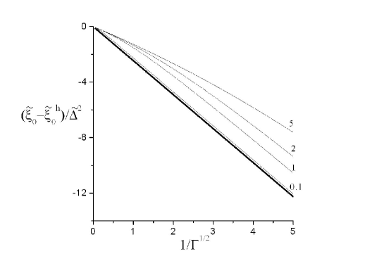
Figure 1: Shift $(\widetilde{\xi}_{0}^{tr}-\widetilde{\xi}_{H}^{tr})/\widetilde{\Delta}^{2}$ of the adsorption-desorption transition point for RHPs with exponentially decaying sequence correlations compared to that of homopolymers, vs. correlation parameter $1/\Gamma^{1/2}$, according to Eq. (47). The different curves show the results for different values of $\widetilde{z_{0}}$ as indicated.

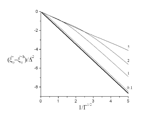
Figure 2: Same as Fig. 1, but for oscillating sequence correlations.

The expressions (47) and (48) demonstrate that the mean affinity parameter ($\widetilde{\xi_{0}}$) corresponding to the adsorption transition is reduced for RHPs, compared to homopolymers. In other words, RHPs have a better effective affinity to surfaces than homopolymers with the same mean affinity.

Our result also shows that the surface affinity of RHPs with exponentially decaying correlations is higher than that of RHPs with oscillating correlations. This can be seen by rewriting the general expression (48) for the particular cases of purely exponential decay ($\Gamma\in\mathbb{R}$)

$$\widetilde{\xi_{0}}^{tr}-\widetilde{\xi_{H}}^{tr}=-{\widetilde{\Delta}}^{2}\sqrt{\frac{6}{\Gamma}}\>,\>\Gamma\in\mathbb{R}$$ (49)

and purely oscillating correlations ($\Gamma\in i\mathbb{R}$)

$$\widetilde{\xi_{0}}^{tr}-\widetilde{\xi_{H}}^{tr}=-{\widetilde{\Delta}}^{2}\sqrt{\frac{3}{\Gamma^{\prime}}}\>,\Gamma=i\,\Gamma^{\prime},\>\Gamma^{\prime}\in\mathbb{R}.$$ (50)

III Numerical Approach

In the previous section, we have developed an analytical theory of RHP adsorption based on the reference system approach, and subobtained as a main result the adsorption-desorption phase diagram, Eqs. (47) and (48) and Fig. 1. To assess directly the validity of the reference system approach, and to test our final result, Eq. (48), we have also performed numerical calculations based on a simple lattice model, following the method of Scheutjens and Fleer PolInterfaces .

III.1 Lattice Model

In the model we use for the numerical calculations, polymer chains of $N$ monomers are represented by random walks of length $N$ on the simple cubic lattice. We consider polymers which have one end tethered to an impenetrable planar surface. In the $z$-direction perpendicular to the plane, the center of mass of a monomer can have coordinates $z=0,l,2l,3l\ldots$, where the layer $z=0$ is directly adjacent to the adsorbing plane. The adsorption potential is taken to be short-ranged and sequence-dependent and has the following form

$$\frac{u_{i}\left(z,i\right)}{kT}=\left\{\begin{array}[]{ll}\chi_{M_{i}}&\mbox{if }z=0\\ 0&\mbox{if }z>0\end{array},\right.$$ (51)

i. e., it acts only on the monomers in the layer that is adjacent to the adsorbing surface. In Eq. (51) $M_{i}$ denotes the type of the $i$-th monomer in the chain and $\chi_{M}$ is the adsorption interaction parameter for monomers of the type $M$. Note that we consider the simplest case of a phantom chain, hence the monomers do not interact with each other and the local monomer potential $u_{i}\left(z,i\right)$ does not depend on the local polymer concentration.

One immediately notices one important difference between this system and the model considered in the previous section: Up to now we have considered free chains, whereas we now study tethered chains. However, within the ground state dominance approximation used to treat chain ends in the last section, the final result for the adsorption transition will be identical for tethered chains and for free chains. Tethering the chains in the numerical calculations helps to avoid an uncertainty with the normalization, because for free chains of finite length one would have to introduce a box of finite size.

We consider two-letter RHP sequences constructed by first order Markov chains ($M_{s}=A,B$). The underlying Markov process is determined by the probabilities to find single A and B monomers ($f_{A}$ and $f_{B}=1-f_{A}$, respectively), and by the nearest-neighbor transition probabilities $p_{i\rightarrow j}$ which is the probability that a monomer $i$ is followed by a monomer $j$. It is convenient to introduce the correlation parameter

$$C=1-p_{A\rightarrow B}-p_{B\rightarrow A}$$ (52)

that characterizes the correlations in the sequence. In the case $C=0$ one has polymers with uncorrelated monomer sequences (Bernoullian type), at $C>0$ the probability to encounter nearest-neighbors of the same type is enhanced, and at $C<0$ nearest-neighbor monomers are more likely to be of different type (as in alternating copolymers). The statistical distribution of the sequences is completely determined by the two parameters $f_{A}$ and $C$.

In the actual calculations, A monomers were always considered as adsorbing or sticky ($\chi_{A}$ is positive), whereas monomers of the B type were taken to be either neutral ($\chi_{B}$ = 0) or repelling from the surface ($\chi_{B}=-\chi_{A}$). These two cases will be referred to as SN (sticker-neutral) or SR (sticker-repulsive).

III.2 Numerical Method

The statistical weight $G_{t}(z;N)$ of all conformations of tethered chains with one free end in the layer $z$ satisfies the following recurrent relation first introduced by Rubin Rubin and later used in the more general theory of Scheutjens and Fleer PolInterfaces

$$\begin{split}G_{t}(z;N+1)=&\left\{\lambda G_{t}(z-1;N)+(1-2\lambda)G_{t}(z;N)\right.\\ &\left.+\>\lambda G_{t}(z+1;N)\right\}\end{split}$$ (53)

$$G_{t}(0;N+1)=\exp(\chi_{M_{i}})\left\{(1-2\lambda)G_{t}(0;N)+\lambda G_{t}(1;N)\right\},$$ (54)

where $\lambda$ is the probability that a random walk step connects neighboring layers. On simple cubic lattices, one has $\lambda=\frac{1}{6}$. Using as the starting point the monomer segment distribution $G(0;1)=\exp(\chi_{M_{i}})$ and recursively applying Eq. (53), one can easily calculate $G_{t}(z;N)$ for every chain length $N$. The statistical weight of all conformations of tethered chains is then obtained by summing over all positions of the free end:

$$Z=\sum_{z=0}^{Nl}G(z;N)$$ (55)

The change in the free energy of the tethered chain with respect to the free chain in the solution is given by $\Delta F=-\log Z$. Here the translational entropy of the free chain has been disregarded, i. e., the chains are assumed to be sufficiently long that it can be neglected. At the transition point one has $\Delta F=0$, i. e., the energetic benefit of monomer-surface contacts is equal to the entropic penalty connected with the fact that tethering the chain at the plane restricts the number of conformations available to the chain.

In order to calculate conformational characteristics of the adsorbed chain, one needs to evaluate not only $G_{t}(z;n)$ for arbitrary $n=1,2,...,N$, but also a second set of functions $G_{f}(z;N-n)$, which gives the statistical weight of chain parts between the $n$th monomer and the end monomer $N$, subject to the constraint that the monomer $n$ is fixed in the layer $z$ (whereas the end monomer is free). To calculate $G_{f}(z;N-n)$ one uses the same recurrence relations as in Eqs. (53) and (54), but with reverted copolymer sequence and different initial conditions $G(z;1)=e^{\left.-u_{N}\left(z\right)\right/kT}$. Combining $G_{t}$ and $G_{f}$ one can then calculate, for example, the average fraction of A contacts with the surface

$$s_{A}=\frac{1}{\mathcal{N}}\sum_{i=1}^{N}G_{t}(0;i)G_{f}(0;N-i+1)\exp(\chi_{M_{i}})\delta_{M_{i},A}.$$ (56)

Here $\delta_{M_{i},A}=1$ if $M_{i}=A$ or 0 otherwise, and the exponential factor is used to correct for the double contribution of the $i$-th monomer. The normalization constant $\mathcal{N}$ is given by

$$\mathcal{N}=\sum_{z=0}^{N-1}\sum_{i=1}^{N}G_{t}(z;i)G_{f}(z;N-i+1)e^{\left.u_{s}\left(z\right)\right/kT}\delta_{M_{s},A}.$$ (57)

The total fractions of A and B contacts can be obtained via

$$s=\frac{1}{\mathcal{N}}\sum_{i=1}{N}G_{t}(0;i)G_{f}(0;N-i+1)e^{\left.u_{s}\left(0\right)\right/kT}.$$ (58)

In this paper, we present results for chains of length $N=500$. For every set of model parameters $f_{A}$ and $C$, the adsorption characteristics were calculated as a function of the interaction parameter $\chi_{A}$ for 50 different sequence realizations and then averaged. This corresponds to a situation with quenched sequence disorder. In contrast, the method developed by van Lent and Scheutjens vanLent describes copolymers with annealed disorder.

A full account of the numerical results will be given elsewhere. In the present paper, we are mostly interested in the comparison with the analytical theory, and in particular, in the two questions that are discussed in the next section.

IV Comparison of the Two Approaches

IV.1 Is the reference system approach valid?

Introducing the reference homopolymer system in Section II.2, we have assumed that its conformational and thermodynamic properties are reasonably close to those of the original RHP system. Later, the optimal value of variational parameter $v_{0}$ has been chosen according to the requirement that it minimizes the free energy difference between the original and the reference systems (43). Therefore, the free energies of the two systems are automatically close. However, one cannot be sure that this choice of $v_{0}$ guarantees good correspondence between the conformational characteristics. This shall be tested first.

One of the most important and indicative conformational property of the adsorbed chain is undoubtedly the total fraction $s$ of adsorbed monomer units. It is plotted in Fig. 3 for RHPs with different composition and structure, and for homopolymers with the same free energy. One can see that near the adsorption transition ($\Delta F=0$), the value of $s$ for RHPs is close to that for homopolymers. The “worst” RHPs are those which contain a majority of surface-repelling monomers. In the strong adsorption regime, however, the values of $s$ differ considerably.

Figure 3: Fraction $s$ of adsorbed segments for homopolymer and RHPs of different type (SN or SR) and composition ($f_{A}$) as a function of the free energy. For each of RHP type and composition curves for $C=0,0.25,0.5$ and 0.75 are shown.

This observation can be explained by the fact that in the vicinity of the transition point, chains have relatively few surface contacts and long loops and tails. Such conformations can be realized equally easily by both homopolymers and RHPs, in spite of the ”gaps” of neutral or repelling monomers in the RHPs. Since only few units adsorb to the surface, the system can avoid entropically and energetically unfavorable contacts of neutral/repelling units with the surface. In the strong adsorption regime, it is thermodynamically more favorable for homopolymers to have many contacts with the surface. This is not necessarily the case for RHPs, because non-adsorbing monomer units still avoid to get involved in the interactions with the surface.

In the strong adsorption regime, the reference system approach of section II.2 thus becomes questionable. However, it seems to be applicable in the vicinity of the transition, and should therefore be suitable to study the transition point.

IV.2 Is the analytically predicted phase diagram correct?

Next we check the scaling relation, Eq. (48), describing the shift of the adsorption transition point of RHPs relative to homopolymers.

To compare Eq. (48) with the numerical results, we need to do two things: (1) find the transition points for lattice RHPs with different composition and ”structure” and (2) ”translate” these results into of parameters of the continuum model parameter ($\widetilde{\xi_{0}}$, $\widetilde{\Delta}$, and $\Gamma$).

The transition point $\chi_{A}^{tr}$ in the lattice model was determined numerically from the condition $\Delta F=0$ for every single realization of a RHP. Then the average over the values $\chi^{tr}$ was performed.

The next step is to find the relation between the statistical parameters of the continuous model and the discrete lattice model. For homopolymer systems this problem has been solved by Gorbunov et al. mapping . According to this work, the coefficient connecting the continuous and the discrete polymerization degree is unity, and the length $a$ in the continuum model corresponds to the lattice spacing $l$ in the case of a simple cubic lattice. To find the mapping for $\widetilde{\xi_{0}}$, $\widetilde{\Delta}$, and $\Gamma$, we calculate the mean monomer-surface interaction parameter

$$\chi_{0}=f_{A}\chi_{A}+(1-f_{A})\chi_{B}$$ (59)

and the monomer-monomer correlation function in terms of the monomer interaction energy. The calculation is straightforward and yields

$$\begin{split}c_{\chi}(n)\equiv&\langle\left(\chi(x)-\chi_{0}\right)\left(\chi(x+n)-\chi_{0}\right)\rangle\\ =&C^{n}f_{A}(1-f_{A})(\chi_{A}-\chi_{B})^{2}.\end{split}$$ (60)

If we represent the correlation function in an exponential form like (4)

$$c_{\chi}(n)=\Delta_{\chi}^{2}\exp\left(-\Gamma_{\chi}n\right),$$

we obtain the equivalent parameters $\Delta$ and $\Gamma$

$$\Gamma_{\chi}=-\log(C)$$ (61)

$$\Delta_{\chi}=\left(\chi_{A}-\chi_{B}\right)\sqrt{f_{A}(1-f_{A})}.$$ (62)

Since the units for the polymerization degree are the same in both models, this yields $\Gamma=\Gamma_{\chi}$.

The two remaining parameters $\widetilde{\xi}_{0}$ and $\widetilde{\Delta}$ are related to the monomer-surface affinity. The mapping of this “energy scale” is much less straightforward. We shall adopt a procedure suggested in Ref. mapping, and adjust the energy scale such that the slope of the monomer density profiles of adsorbed homopolymers at the surface is the same in the vicinity of the adsorption transition. Comparing Eq. (15) of Ref. mapping, with the $z_{0}\to 0$ limit of Eq. (31), we obtain

$$\frac{\widetilde{\xi}_{H}-\widetilde{\xi}^{tr}_{H}}{\chi_{H}-\chi^{tr}_{H}}=\frac{5}{6}$$ (63)

for homopolymers on simple cubic lattices. We assume that the factor (5/6) thus relates the energy scales in our two models, i. e., the continuum model and the lattice model. Thus we conclude

$$\frac{\widetilde{\xi}^{tr}_{0}-\widetilde{\xi}^{tr}_{H}}{\chi^{tr}_{0}-\chi^{tr}_{H}}=\frac{\widetilde{\Delta}}{\Delta_{\chi}}=\frac{5}{6}.$$ (64)

The approach has the drawback of being rather indirect. Moreover, the energy mapping applies, if at all, only in the close vicinity of the transition point.

Inserting these relations for $\widetilde{\xi}_{0}$, $\Gamma$, and $\widetilde{\Delta}$ into Eq. (48) we obtain the following relation between equivalent lattice parameters

$$\chi_{0}^{tr}-\chi^{tr}_{H}=-\Delta_{\chi}^{2}\frac{5}{\sqrt{6\Gamma}}$$ (65)

Thus $\chi_{0}^{tr}-\chi^{tr}$ is expected to depend linearly on $\Delta_{\chi}^{2}/\sqrt{\Gamma}$, with a slope $-5/\sqrt{6}\approx-2.04$.

The results for $\chi_{0}^{tr}-\chi^{tr}_{H}$ are shown in Fig. 4. One can see that the numerical calculations reproduce well the expected linear dependence between $\chi_{0}^{tr}-\chi^{tr}_{H}$ and $\Delta_{\chi}^{2}/\sqrt{\Gamma}$. However, the slope ($\approx-0.754$) is different from that predicted by Eq. (65).

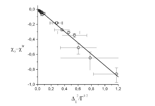
Figure 4: Shift $\chi^{tr}_{0}-\chi_{H}^{tr}$ of the adsorption transition in RHP systems relative to homopolymer systems for the lattice model vs. $\Delta_{\chi}^{2}/\Gamma^{1/2}$. The solid line shows the best linear fit.

V Conclusions

To summarize, we have studied the adsorption of single ideal heteropolymer chains onto homogeneous planar surfaces. After applying the replica trick we have introduced a reference homopolymer system chosen such that the thermodynamic properties were as close as possible to those of the original RHP system. This approach allowed us to treat the problem analytically and to obtain the adsorption-desorption phase diagram of the RHP. In particular, we have considered the case of RHPs with primary sequence correlations described by a de-Gennes correlator. We found that the adsorption is enhanced with increasing strength of correlation ($\Delta$) and correlation length ($1/\Gamma$), both for the cases of decaying and oscillating correlations. Our result could be summarized in a very simple equation for the shift of the adsorption transition in correlated RHPs relative to homopolymers, Eq. (48).

To test the reference system approach, numerical lattice calculations were performed. These results show that in the vicinity of the transition point, our variational is well justified. Furthermore, the calculation of the adsorption-desorption phase diagram confirmed the analytical scaling prediction. However, we also found that far from the transition point, one cannot ”construct” a reference homopolymer system that is good in both a conformational and a thermodynamical sense. A reference system perhaps more adequate to describe this case could be a multiblock-copolymer system with block lengths equal to the average length of A and B blocks in the random copolymers. In the lattice model, these are equal to $s_{A}=1/[(1-f_{A})(1-c)]$ and $s_{B}=1/[f_{A}(1-c)]$, respectively rcp_stat ). This could be interesting for future work.

We found that our main result, Eq. (48), describes the numerical result very satisfactorily from a qualitative point of view. Unfortunately, true quantitative agreement could not yet be established. The reason lies partly in the fact that the identification of energy scales in the lattice model and in the continuum model is not self evident. We have tested a mapping procedure which adjusts the monomer profiles for adsorbed homopolymers. Within this approach, the theory seems to overestimate the shift of the adsorption transition in RHP systems. However, the mapping can be questioned, as we have discussed in the last section. Furthermore, we are comparing a theory for RHPs with continuous (Gaussian distributed) monomers with numerical calculations for two-letter RHPs, which might also lead to problems.

Acknowlegdement

The financial support of the Deutsche Forschungsgemeinschaft (SFB 613) is gratefully acknowledged.

Appendix: Calculation of $\mathcal{G}(z_{0},z_{0};p)$

Our starting point is Eq. (18) with the initial condition (19) and the boundary conditions (20). Laplace transforming with respect to $N$ gives

$$-p\mathcal{G}(z,z^{\prime};p)+G(z,z^{\prime};0)=-\frac{a^{2}}{6}\frac{\partial^{2}\mathcal{G}}{\partial z^{2}}-\beta w_{0}\delta(z-z_{0})\mathcal{G}(z,z^{\prime};p),$$ (66)

where $\mathcal{G}(z,z^{\prime};p)$ is the Laplace transform of $G(z,z^{\prime};N)$ with respect to $N,$ $\mathcal{G}(z,z^{\prime};p)=\int_{0}^{\infty}G(z,z^{\prime};N)e^{-pN}dN$. Taking into account the initial condition (19), we obtain

$$-p\mathcal{G}(z,z^{\prime};p)+\delta(z-z^{\prime})=-\frac{a^{2}}{6}\frac{\partial^{2}\mathcal{G}}{\partial z^{2}}-\beta w_{0}\delta(z-z_{0})\mathcal{G}(z,z^{\prime};p)$$ (67)

with the boundary conditions

$$\mathcal{G}(z,z^{\prime};p)|_{z\to\infty}=0,\quad\mathcal{G}(z,z^{\prime};p)|_{z\to 0}=0$$ (68)

Laplace transforming (67) with respect to $z$ with (20) gives

$$-pg(s,z^{\prime};p)+e^{-z^{\prime}s}=-\frac{a^{2}}{6}\left[s^{2}g(s,z^{\prime};p)-s\mathcal{G}(0,z^{\prime};p)-\mathcal{G}^{\prime}(0,z^{\prime};p)\right]-\beta w_{0}\mathcal{G}(z_{0},z^{\prime};p)e^{-z_{0}s}$$

where $g(s,z^{\prime};p)$ is the Laplace transform of $\mathcal{G}(z,z^{\prime};p)$ with respect to $z$, $g(s,z^{\prime};p)=\int_{0}^{\infty}\mathcal{G}(z,z^{\prime};p)e^{-sz}dz$, and $\mathcal{G}^{\prime}$ stands for $\partial\mathcal{G}/\partial z$. With the boundary condition at $z=0$ (68) we obtain

$$-pg(s,z^{\prime};p)+e^{-z^{\prime}s}=-\frac{a^{2}}{6}\left[s^{2}g(s,z^{\prime};p)-\mathcal{G}^{\prime}(0,z^{\prime};p)\right]-\beta w_{0}\mathcal{G}(z_{0},z^{\prime};p)e^{-z_{0}s}$$ (69)

Solving this equation for $g(s,z^{\prime};p)$ yields

$$g(s,z^{\prime};p)=\frac{\mathcal{G}^{\prime}(0,z^{\prime};p)-(6\beta w_{0}/a^{2})\mathcal{G}(z_{0},z^{\prime};p)e^{-z_{0}s}-(6/a^{2})e^{-z^{\prime}s}}{s^{2}-(6p/a^{2})}$$ (70)

Taking the inverse Laplace transform of (70) with respect to $s$ gives

$$\begin{split}\mathcal{G}(z,z^{\prime};p)=\frac{a}{\sqrt{6p}}&\left\{\sinh\left(\sqrt{6p}\,\frac{z}{a}\right)\,\mathcal{G}^{\prime}(0,z^{\prime};p)\right.-\frac{6\beta w_{0}}{a^{2}}\,\sinh\left(\sqrt{6p}\,\frac{z-z_{0}}{a}\right)\,\mathcal{G}(z_{0},z^{\prime};p)\,\theta(z-z_{0})\\ &\left.-\frac{6}{a^{2}}\sinh\left(\sqrt{6p}\,\frac{z-z^{\prime}}{a}\right)\,\theta(z-z^{\prime})\right\},\end{split}$$ (71)

where $\theta(z)$ is the Heaviside function

$$\theta(z)=\left\{\begin{aligned} &1\mbox{, if }z>0\\ &0\mbox{, if }z<0\end{aligned}\right..$$

Setting $z=z_{0}$ in Eq. (71), we obtain

$$\mathcal{G}(z_{0},z^{\prime};p)=\,\frac{a}{\sqrt{6p}}\left\{\sinh\left(\sqrt{6p}\,\frac{z_{0}}{a}\right)\,\mathcal{G}^{\prime}(0,z^{\prime};p)-\frac{6}{a^{2}}\sinh\left(\sqrt{6p}\,\frac{z_{0}-z^{\prime}}{a}\right)\,\theta(z_{0}-z^{\prime})\right\}$$ (72)

and then insert $\mathcal{G}(z_{0},z^{\prime};p)$ back into Eq. (71) (second term):

$$\begin{split}\mathcal{G}(z,z^{\prime};p)&=\frac{a}{\sqrt{6p}}\left\{\sinh\left(\sqrt{6p}\,\frac{z}{a}\right)\,\mathcal{G}^{\prime}(0,z^{\prime};p)-\frac{6\beta w_{0}}{a^{2}}\,\sinh\left(\sqrt{6p}\,\frac{z-z_{0}}{a}\right)\,\theta(z-z_{0})\right.\\ &\times\frac{a}{\sqrt{6p}}\left[\sinh\left(\sqrt{6p}\,\frac{z_{0}}{a}\right)\,\mathcal{G}^{\prime}(0,z^{\prime};p)-\frac{6}{a^{2}}\sinh\left(\sqrt{6p}\,\frac{z_{0}-z^{\prime}}{a}\right)\,\theta(z_{0}-z^{\prime})\right]\\ &\left.-\frac{6}{a^{2}}\sinh\left(\sqrt{6p}\,\frac{z-z^{\prime}}{a}\right)\,\theta(z-z^{\prime})\right\}\end{split}$$ (73)

To find the unknown $\mathcal{G}^{\prime}(0,z^{\prime};p)$, we require $\mathcal{G}(z\to\infty,z^{\prime};p)$ to vanish and $z^{\prime}$ to be finite. This implies that the coefficient of the growing term term $e^{\sqrt{6p}z/a}$ must be zero. Using (73), this requirement leads to the following result for $\mathcal{G}^{\prime}(0,z^{\prime};p)$:

$$\mathcal{G}^{\prime}(0,z^{\prime};p)=\frac{6}{a^{2}}\>\frac{{e^{-\sqrt{6p}z^{\prime}/a}-\frac{6\beta w_{0}}{a^{2}}\frac{a}{\sqrt{6p}}\sinh\left(\sqrt{6p}\,\frac{z_{0}-z^{\prime}}{a}\right)e^{-\sqrt{6p}z_{0}/a}\theta(z_{0}-z^{\prime})}}{1-\frac{6\beta w_{0}}{a^{2}}\frac{a}{\sqrt{6p}}\sinh\left(\sqrt{6p}\,\frac{z_{0}}{a}\right)e^{-\sqrt{6p}z_{0}/a}}$$ (74)

To find $\mathcal{G}(z_{0},z_{0};p)$, we substitute (74) into (73) and set $z=z_{0}$ and $z^{\prime}=z_{0}$. The result is

$$\begin{split}\mathcal{G}(z_{0},z_{0};p)&=\frac{a}{\sqrt{6p}}\>\frac{6}{a^{2}}\>\frac{\sinh\left(\sqrt{6p}\,z_{0}/a\right)}{e^{\sqrt{6p}z_{0}/a}-\frac{6\beta w_{0}}{a^{2}}\frac{a}{\sqrt{6p}}\sinh\left(\sqrt{6p}\,z_{0}/a\right)}\\ &=\frac{\sinh\left(\sqrt{6p}\,z_{0}/a\right)}{a\sqrt{p/6}\>e^{\sqrt{6p}z_{0}/a}-\beta w_{0}\sinh\left(\sqrt{6p}\,z_{0}/a\right)}\end{split}.$$ (75)

References

- (1) J.-F. Joanny, J. Phys. II (France) 101, 1281 (1994).
- (2) L. Gutman and A. Chakraborty, J. Chem. Phys. 103, 10733 (1995).
- (3) L. Gutman and A. Chakraborty, J. Chem. Phys. 101, 10074 (1994).
- (4) S. Stepanow and A. L. Chudnovsky, J. Phys. A 35, 4229 (2002).
- (5) K. Sumithra and A. Baumgaertner, J. Chem. Phys. 110, 2727 (1999).
- (6) M. S. Moghaddam and S. G. Wittington, J. Phys. A: Math. Gen. 35, 33 (2002).
- (7) B. van Lent and J. M. H. M. Scheutjens, J. Phys. Chem. 94, 5033 (1990).
- (8) E. A. Zheligovskaya, P. G. Khalatur, and A. R. Khokhlov, Phys. Rev. E 59, 3071 (1999).
- (9) A. Chakraborty and D. Bratko, J. Chem. Phys. 108, 1676 (1998).
- (10) A. Chakraborty, Phys. Rep. 342, 1 (2001).
- (11) S. Srebnik, A. Chakraborty, and E. I. Shakhnovich, Phys. Rev. Lett. 77, 3157 (1996).
- (12) D. Bratko, A. Chakraborty, and E. I. Shakhnovich, Comp. Theor. Polym. Sci. 8, 113 (1998).
- (13) D. Bratko, A. Chakraborty, and E. I. Shakhnovich, Chem. Phys. Lett. 280, 46 (1997).
- (14) N. A. Denesyuk and I. Ya. Erukhimovich, J. Chem. Phys. 113, 3894 (2000).
- (15) Z. Y. Chen, J. Chem. Phys. 112, 8665 (2000).
- (16) P.-G. de Gennes, Faraday Discuss. Chem. Soc. 68, 96 (1979).
- (17) M. Doi, S. F. Edwards, The Theory of Polymer Dynamics (Oxford Univ. Press, New York, 1986).
- (18) P.-G. de Gennes, Scaling Concepts in Polymer Physics (Cornell Univ. Press, Ithaca, 1979).
- (19) P.-G. de Gennes, Rep. Prog. Phys. 32, 187 (1978).
- (20) Y. Lépine Y. and A. Caillé, Can. J. Phys. 56, 403 (1969).
- (21) C. Aslangul, Am. J. Phys. 63, 935 (1995).
- (22) G. J. Fleer, M. A. Cohen-Stuart, J.M.H.M Scheutjens, T. Cosgrove, and B. Vincent, Polymers at Interfaces (Chapman and Hall, London, 1993).
- (23) R. J. Rubin, J. Res. Natl. Bur. Stand. Sec. B 69, 301 (1965); 70, 237 (1966); J. Chem. Phys. 43, 2392 (1965).
- (24) A. A. Gorbunov, A. M. Skvortsov, J. van Male, and G. J. Fleer, J. Chem. Phys. 114, 5366 (2001).
- (25) N. Striebeck, Polymer 33, 2792 (1992); G. G. Odian, Princples of Polymerisation (Wiley, New York, 1991).