Semiconductor Microstructure in a Squeezed Vacuum:
Electron-Hole Plasma Luminescence

Abstract

We consider a semiconductor quantum-well placed in a wave guide microcavity and interacting with the broadband squeezed vacuum radiation, which fills one mode of the wave guide with a large average occupation. The wave guide modifies the optical density of states so that the quantum well interacts mostly with the squeezed vacuum. The vacuum is squeezed around the externally controlled central frequency $\omega_{0}$, which is tuned above the electron-hole gap $E_{g}$, and induces fluctuations in the interband polarization of the quantum-well. The power spectrum of scattered light exhibits a peak around $\omega_{0}$, which is moreover non-Lorentzian and is a result of both the squeezing and the particle-hole continuum. The squeezing spectrum is qualitatively different from the atomic case. We discuss the possibility to observe the above phenomena in the presence of additional non-radiative (e-e,  phonon) dephasing.

I Introduction

The modification of the spontaneous emission of an atom placed in a cavity has been predicted and observed a long time ago Kleppner81 ; goy . Recently, cavity effects have been observed also in quantum dots and quantum wells Solomon which were placed in a microcavity made of Distributed Bragg Mirrors (DBRs). Similarly, effects of non-classical radiation, such as squeezed vacuum states produced in the process of parametric down-conversion, were considered in the context of interaction with atoms Gardiner86 ; Palma-Knight ; Charmichael87 . An important theoretical prediction was made by Gardiner Gardiner86 , that an atom coupled to a squeezed reservoir will exhibit two line widths in its resonance fluorescence spectrum. To observe this effect, it is necessary that most of the electromagnetic modes which are resonant with the atomic transition are occupied by squeezed vacuum with a large average photon occupation.

In this letter we consider the coupling of a two-band system of a semiconductor quantum well to a squeezed reservoir of photons occupying the modes of an ideal optical wave guide (without leakage). This presents a generalization of the atomic case in several ways: (1) there is a continuum of electron-hole excitations in the band, (2) each particle-hole excitation is detuned differently with respect to the squeezing energy $\omega_{0}$ (which is externally controlled), (3) inevitable additional nonradiative relaxation and dephasing. The solid-state environment involves more types of interactions which have to be considered together, but it offers a possibility to observe these quantum optical effects, as the quality of cavities improves. Specifically, we consider the luminescence of the scattered squeezed state, in the regime where the nonradiative dephasing ($\gamma_{2}$) is of the order or smaller than the radiative transition rate ($\Gamma$), and the relaxation ($\gamma_{1}$) of electrons is small compared to $\Gamma$. In this regime, where the radiation may be assumed to be a reservoir, we will argue that the effect of Coulomb interaction is mainly to give rise to dephasing. We calculate the optical spectra of the unshifted luminescence, i.e. the scattered radiation with the same frequency as the incoming radiation and compare it qualitatively to the atomic case. The power spectrum (Fig. 1) has a non-Lorentzian peak at the frequency $\omega_{0}$, a consequence of the strong energy dependence of the correlation times of the fluctuating polarization of different e-h pairs. The squeezing spectrum exhibits reduced fluctuations in one quadrature (Fig. 2), the minimum of which is proportional to $\sqrt{\Gamma+\gamma_{2}-|\Lambda|}$, where $\Lambda$ is a measure of the squeezing correlations of the field.

II Model

We will first present our model system and the results for the scattered radiation, and later discuss its possible realization. The free part of the Hamiltonian $H=H_{0}+H_{I}+H_{c}$ is given by ($\hbar\equiv 1$)

$$H_{0}=\sum_{\lambda q}\omega_{\lambda q}b^{\dagger}_{\lambda q}b_{\lambda q}+\sum_{k}\epsilon_{k}^{c}c^{\dagger}_{k}c_{k}+\sum_{k}\epsilon_{k}^{v}v^{\dagger}_{k}v_{k}.$$ (1)

The operators $c_{k}$ and $v_{k}$ denote annihilation operators of the free electrons in the conduction and valence bands of the quantum well, with in-plane momentum $k$ (omitting spin). The operators $b_{\lambda q}$ denote the photon annihilation operators of the wave guide mode $\lambda$ with wave number $q$. For simplicity we confine ourselves to the case of normal incidence, i.e. $q$ is orthogonal to the electronic in-plane momentum $k$. The interaction of the electrons and the photons in the dipole approximation is given by Haug-Koch-Book ; Khitrova-Review

$$H_{I}=\sum_{k\lambda q}\mathcal{E}(\omega_{\lambda q})u_{\lambda}b_{\lambda q}(d_{cv}c^{\dagger}_{k}v_{k}+d^{*}_{cv}v^{\dagger}_{k}c_{k})+\,\,\,h.c.$$ (2)

where $\mathcal{E}(\omega_{\lambda q})=\sqrt{\frac{\omega_{\lambda q}}{V}}$, $u_{\lambda}$ is an overlap integral of the electronic envelope and wave guide mode functions, $d_{cv}$ is dipole matrix element (we suppress its weak dependence on $k$ ), and $V$ is the wave guide volume. Finally, the Coulomb interaction is given by Haug-Koch-Book

$$H_{c}=\frac{1}{2}\sum_{k,k^{\prime},q\neq 0}U_{q}\left(2c^{\dagger}_{k+q}v^{\dagger}_{k^{\prime}-q}v_{k^{\prime}}c_{k}+\right.$$ (3)

$$\left.+c^{\dagger}_{k+q}c^{\dagger}_{k^{\prime}-q}c_{k^{\prime}}c_{k}+v^{\dagger}_{k+q}v^{\dagger}_{k^{\prime}-q}v_{k^{\prime}}v_{k}\right)$$

where $U_{q}$ is the bare Coulomb interaction.

We assume that the radiation acts as a reservoir with correlations of a two mode broadband squeezed vacuum Gardiner86

$$\langle b^{\dagger}_{\lambda q}b_{\lambda^{\prime}q^{\prime}}\rangle=\mathcal{N}(\omega_{\lambda q})\delta_{\lambda\lambda^{\prime}}\delta(\omega_{\lambda q}-\omega_{\lambda q^{\prime}})$$ (4)

$$\langle b_{\lambda q}b_{\lambda^{\prime}q^{\prime}}\rangle=\mathcal{M}(\omega_{\lambda q})\delta_{\lambda\lambda^{\prime}}\delta(2\omega_{0}-\omega_{\lambda q}-\omega_{\lambda q^{\prime}})$$

$$\langle b_{\lambda q}\rangle=0$$

where $\mathcal{N}(\omega_{\lambda q})$ is the average photon occupation of the mode $\lambda$ and wave number $q$, and $\mathcal{M}(\omega_{\lambda q})$ is the squeezing parameter Gardiner86 . We assume that $\mathcal{N},\,\mathcal{M}\gg 1$ within the bandwidth $\omega_{0}\pm B/2$ of one squeezed mode (denoted by $\lambda=s$) and they vanish for other empty modes (denoted by $\lambda=e$).

The energy of the central frequency $\omega_{0}$ is tuned higher than the electron-hole gap $E_{g}$, and the bandwidth of the squeezed radiation ($B$) is assumed to be much larger than the radiative width ($\Gamma$), but much smaller than the conduction band width. The radiation induces interband transitions between the valence and conduction bands. In principle, when the photon occupation is large, it is possible to find the system in a regime where the dephasing rates due to non-radiative and radiative scattering are comparable, and nonradiative relaxation is small. In this regime the system, initially an unexcited full valence band, reaches a stationary state in which there is a large occupation of the conduction band in the energy stripe where the photon occupation is large.

In order to understand qualitatively the effect of the squeezed reservoir on the electron-hole pair, it is instructive to begin with the equation of motion for $\langle P^{\dagger}_{k}(t)\rangle=\langle c^{\dagger}_{k}(t)v_{k}(t)\rangle$, the interband polarization, without taking into account explicitly the $H_{c}$ part of the Hamiltonian. Using the Markov approximation Haug-Koch-Book we find in the rotating frame of frequency $\Delta\epsilon_{k}=\epsilon^{c}_{k}-\epsilon^{v}_{k}$,

$$\frac{d\langle P^{\dagger}_{k}(t)\rangle}{dt}=-(\Gamma+\gamma_{2})\langle P^{\dagger}_{k}(t)\rangle+e^{2i\delta_{k}t}\Lambda\langle P_{k}(t)\rangle$$ (5)

where $\delta_{k}=\omega_{0}-\Delta\epsilon_{k}$ is the detuning frequency, $\gamma_{2}$ is the dephasing rate due to electron-electron and electron-phonon scattering. The radiative decay coefficients $\Gamma$ and $\Lambda$ are given (for the squeezed mode $\lambda=s$) by

$$\Gamma(\Delta\epsilon_{k})=\rho(\Delta\epsilon_{k})|A_{s}(\Delta\epsilon_{k})|^{2}(\mathcal{N}(\Delta\epsilon_{k})+\frac{1}{2})$$ (6)

$$\Lambda(\Delta\epsilon_{k})=\rho(\Delta\epsilon_{k})\mathcal{M}(\Delta\epsilon_{k})A_{s}^{*}(\Delta\epsilon_{k})A_{s}^{*}(2\omega_{0}-\Delta\epsilon_{k})$$

where $\rho$ is the optical density of states, and $A_{s}(\Delta\epsilon_{k})=\mathcal{E}(\Delta\epsilon_{k})u_{s}d_{cv}$ is the electron-photon coupling strength. It is assumed that there is only a small number of empty resonant modes, thus neglecting their influence in the dynamics of $\langle P^{\dagger}_{k}\rangle$.

The special features of equation (5) are: (1) the coupling of $P^{\dagger}_{k}$ to $P_{k}$, due to the squeezing correlations (Eq. (4)) in the radiation, and (2) the absence of a coupling to the population inversion $\Delta n_{k}=n^{v}_{k}-n^{c}_{k}$, due to the zero average of the field, Eq. (4). The solution of (5) exhibits two complex frequencies

$$\Omega_{1,2}(k)=i(\Gamma+\gamma_{2})+\delta_{k}\mp i\sqrt{|\Lambda|^{2}-\delta_{k}^{2}}.$$ (7)

For $\delta_{k}<|\Lambda|$, the frequencies $\Omega_{1,2}(k)$ have two different imaginary parts, which can be interpreted as over-damping of the polarization, whereas for $\delta_{k}>|\Lambda|$ the $\Omega_{1,2}(k)$ have two different real parts, reminiscent of under-damping.

The incoming squeezed vacuum radiation can not induce average interband polarization. However, it induces fluctuations $\langle P^{\dagger}_{k}(t+\tau)P_{k^{\prime}}(t)\rangle$ and $\langle P_{k}(t+\tau)P_{k^{\prime}}(t)\rangle$ of the polarization, which in turn give rise to scattered radiation in all the resonant wave guide modes. These correlators can be measured by power and squeezing spectra. First we calculate the power spectrum of the scattered radiation into an initially empty mode of the wave guide ($\lambda=e$). In the long-time limit it is given by

$$\mathcal{L}(\omega_{{\lambda q}})\equiv\frac{\partial}{\partial t}N_{e,q}(t)=\sum_{kk^{\prime}}|A_{e}(\omega_{e,q})|^{2}\times$$ (8)

$$\times\int_{-\infty}^{\infty}d\tau e^{-i(\omega_{e,q}-\Delta\epsilon_{k})\tau}\langle P^{\dagger}_{k}(t+\tau)P_{k^{\prime}}(t)\rangle$$

where $N_{e,q}$ is the occupation of the photon mode $\lambda=e$ with wave number $q$.

Let us begin by considering the Coulomb interaction. The effective mean field Hamiltonian lindberg-koch which usually leads to coherent excitonic correlations in the e-h plasma is given by

$$H_{eff}=-\sum_{k,q\neq 0}U_{q}\left(n^{c}_{k-q}c^{\dagger}_{k}c_{k}+n^{v}_{k-q}v^{\dagger}_{k}v_{k}+\right.$$ (9)

$$\left.+p^{*}_{k-q}v^{\dagger}_{k}c_{k}+p_{k-q}c^{\dagger}_{k}v_{k}\right)$$

where $n^{c,v}_{k}$ are band occupations and $p_{k}=\langle P_{k}\rangle$. For the dynamics of $\langle P^{\dagger}_{k}(t+\tau)P_{k^{\prime}}(t)\rangle$ w.r.t. $\tau$, under the condition $p_{k}=0$ this interaction can only induce energy level shifts. Going beyond the mean field approximation it is simplest to consider the equation of motion for the correlations $C_{kk^{\prime}}\equiv\langle P^{\dagger}_{k}(t)P_{k^{\prime}}(t)\rangle$. This equation contains contributions of the form $(1-n^{c}_{k}-n^{v}_{k-q})\sum_{k^{\prime}}U_{k^{\prime}-k}C_{kk^{\prime}}$, which in principle give rise to an excitonic effect . In the presence of the photon reservoir which we consider here, we assume the band occupations $n^{c,v}_{k}$ to be close to $1/2$ (see below), leading to a reduction of the excitonic effect through the phase filling prefactor $(1-n^{c}_{k}-n^{v}_{k-q})$. As a result of the above considerations we will assume from now on that the effect of Coulomb interaction is twofold. First it gives rise to energy shifts which we assume constant over the range $B$, and include in $\epsilon^{(v,c)}_{k}$. Second, it induces dephasing which we assume is included in phenomenological constant $\gamma_{2}$.

Let us turn next to the interaction of the electronic band with the squeezed reservoir. The equation of motion for $\langle P^{\dagger}_{k}(t+\tau)P_{k^{\prime}}(t)\rangle$ with respect to $\tau$ can be derived from the explicit equation of motion for the operator $P^{\dagger}_{k}(t)$ (see appendix), which a form similar to Eq. (5). The solution for $\tau>0$ is given by

$$\langle P^{\dagger}_{k}(t+\tau)P_{k^{\prime}}(t)\rangle=$$ (10)

$$=G_{k}(\tau)\langle P^{\dagger}_{k}(t)P_{k^{\prime}}(t)\rangle+H_{k}(\tau)e^{2i\delta_{k}t}\langle P_{k}(t)P_{k^{\prime}}(t)\rangle$$

where

$$G_{k}(\tau)=\frac{1}{2}\left[e^{i\Omega_{1}(k)\tau}(1-i\frac{\delta_{k}}{\Delta_{k}})+e^{i\Omega_{2}(k)\tau}(1+i\frac{\delta_{k}}{\Delta_{k}})\right]$$

$$H_{k}(\tau)=\frac{\Lambda}{2\Delta_{k}}(e^{i\Omega_{1}(k)\tau}-e^{i\Omega_{2}(k)\tau}).$$ (11)

where $\Delta_{k}=\sqrt{|\Lambda|^{2}-\delta_{k}^{2}}$. For $\tau<0$ the solution is given by taking $G^{*}_{k}(-\tau)$ and $H^{*}_{k}(-\tau)$. The dependence of the last term on $t$ in Eq. (10) is due to the non-stationary nature of the squeezed radiation Gardiner86 .

The off diagonal $k\neq k^{\prime}$ elements of equal time correlations $\langle P^{\dagger}_{k}(t)P_{k^{\prime}}(t)\rangle$ and $\langle P_{k}(t)P_{k^{\prime}}(t)\rangle$ which serve as initial conditions in (10) vanish in equilibrium. However here the system is coupled to two reservoirs: the nonradiative thermal bath and the squeezed reservoir. It can be shown unpublished that as a result there are non-zero steady state off-diagonal correlations of two kinds: normal $\langle P^{\dagger}_{k}(t)P_{k^{\prime}}(t)\rangle$ and anomalous $\langle P_{k}(t)P_{k^{\prime}}(t)\rangle$. They are smaller than the diagonal correlations $\langle P^{\dagger}_{k}(t)P_{k}(t)\rangle$ by a factor proportional to $(\frac{\gamma_{1}}{\Gamma})^{2}$. Qualitatively this can be estimated by referring to the equation $\partial_{t}P_{k}=d_{cv}\sum_{\lambda q}\mathcal{E}(\omega_{\lambda q})u_{\lambda}b_{\lambda q}\Delta n_{k}$. The off diagonal correlations are driven by the squeezed reservoir since there exists a non-zero steady state difference $\langle\Delta n_{k}\rangle$. This is given by the rate equation

$$\partial_{t}\Delta n_{k}(t)=-(\Gamma+\gamma_{1})\Delta n_{k}(t)+\gamma_{1}$$ (12)

which leads to the above estimate.

III Results

We shall treat the luminescence in the limit of $\gamma_{1}/\Gamma\to 0$ so that only the diagonal correlations $\langle P^{\dagger}_{k}(t+\tau)P_{k}(t)\rangle$ contribute to (8). Moreover, since $\langle P_{k}(t)P_{k}(t)\rangle=0$, and $\langle P^{\dagger}_{k}(t)P_{k}(t)\rangle=\langle n^{c}_{k}\rangle\langle 1-n^{v}_{k}\rangle$, Eq. (10) shows that $\langle P^{\dagger}_{k}(t+\tau)P_{k}(t)\rangle$ are stationary in this limit.

Substituting (10) with $k=k^{\prime}$ and (LABEL:fluc-funcs) in the integral (8) we obtain

$$\mathcal{L}(\omega_{\lambda q})=2|A_{\lambda}(\omega_{{\lambda q}})|^{2}Re\int d^{2}k\langle n^{c}_{k}\rangle\langle 1-n^{v}_{k}\rangle\left[\frac{i}{\Delta\epsilon_{k}-\omega_{\lambda q}+\Omega_{1}(k)}(1-i\frac{\delta_{k}}{\Delta_{k}})+\frac{i}{\Delta\epsilon_{k}-\omega_{\lambda q}+\Omega_{2}(k)}(1+i\frac{\delta_{k}}{\Delta_{k}})\right]$$ (13)

where we assume $\lambda=e$ from now on. The lineshape of an individual particle-hole transition (the integrand of (13)) has two distinct limits (see insert of figure (1)): when $\delta_{k}\rightarrow 0$ it consists of two superimposed regular Lorentzian lineshapes of different widths $\Gamma+\gamma_{2}\pm|\Lambda|$. When $\delta_{k}\gg\Lambda$ the lineshape is a single Lorentzian of width $\Gamma+\gamma_{2}$, which is just the radiative width acquired without squeezing. In between those limits the lineshapes are asymmetric with short tails lying on the side of the central frequency $\omega_{0}$. The superposition of such lineshapes produces a non-Lorentzian peak at $\omega_{0}$ in the unshifted luminescence spectrum $\mathcal{L}(\omega_{\lambda q})$, Fig. (1). For simplicity $\langle n_{k}\rangle$, $\mathcal{N}(\Delta\epsilon_{k})$, $A_{\lambda}(\omega_{\lambda q})$ and $\mathcal{M}(\Delta\epsilon_{k})$ were taken as constant in the energy range $\omega_{0}\pm B/2$ (these will be assumed also below for the squeezing spectrum).

The width of the peak is of the order of $\Gamma+\gamma_{2}$, and the maximum is (in the $B\gg\Gamma$ limit)

$$\mathcal{L}_{max}=\mathcal{L}_{0}\frac{\Gamma+\gamma_{2}}{\sqrt{(\Gamma+\gamma_{2})^{2}-|\Lambda|^{2}}},$$ (14)

where $\mathcal{L}_{0}=4\pi^{2}|A_{\lambda}(\omega_{\lambda q})|^{2}\rho_{el}\langle n^{c}_{k}\rangle\langle 1-n^{v}_{k}\rangle$ with $\rho_{el}$ the electronic density of states.

We now turn to the squeezing spectrum which is defined Gardiner-Parkins-Collet in terms of the fluctuations of the field quadrature $X_{\theta}=\frac{1}{2}\left[E^{(+)}(t)e^{i\omega_{0}t-i\theta}+E^{(-)}(t)e^{-i\omega_{0}t+i\theta}\right]$,

$$\mathcal{S}_{\theta}(\omega_{\lambda q})=\int_{-\infty}^{\infty}d\tau\langle:X_{\theta}(t+\tau)X_{\theta}(t):\rangle e^{i\Delta\omega_{\lambda q}\tau}$$ (15)

where $\Delta\omega_{\lambda q}\equiv\omega_{\lambda q}-\omega_{0}$ and $\theta$ determines the choice of quadrature. For the limit $\gamma_{1}\ll\Gamma$ we again neglect the off-diagonal correlations $\langle P_{k}(t)P_{k^{\prime}}(t)\rangle$ ($k\neq k^{\prime}$) and obtain in the long time limit,

$$\mathcal{S}_{\theta}(\omega_{\lambda q})=\frac{1}{2}\psi^{2}Re\int d^{2}k\langle n^{c}_{k}\rangle\langle 1-n^{v}_{k}\rangle\left[\left(1+\frac{|\Lambda|\cos(2\theta+\alpha)}{\Delta_{k}}\right)\frac{-1}{i\Delta\omega_{\lambda q}+\Delta_{k}-(\Gamma+\gamma_{2})}+\right.$$ (16)

$$+\left.\left(1-\frac{|\Lambda|\cos(2\theta+\alpha)}{\Delta_{k}}\right)\frac{-1}{i\Delta\omega_{\lambda q}-\Delta_{k}-(\Gamma+\gamma_{2})}\right]$$

where $\alpha$ is the phase of $\Lambda$, Eq. (6), and $\psi$ is a geometrical factor . Figure (2) shows the squeezing spectra for the in-phase ($2\theta+\alpha=0$) and out-of-phase ($2\theta+\alpha=\pi$) quadratures, normalized to the total emitted power. The minimum of the out-of-phase quadrature is proportional to $\sqrt{\frac{\Gamma+\gamma_{2}-|\Lambda|}{\Gamma+\gamma_{2}+|\Lambda|}}$, and thus can in principle be very small for ideal squeezing ($\Lambda\rightarrow\Gamma$) and vanishing non-radiative dephasing ($\gamma_{2}\rightarrow 0$). Note that the squeezing spectrum is defined with respect to the normally ordered correlation function so that a zero value means reduction to vacuum fluctuations. The squeezing spectrum of a band is qualitatively different from that of a single particle-hole (insert of Fig. (2)), which has a maximum proportional to $\frac{1}{\Gamma+\gamma_{2}+|\Lambda|}$ at $\omega_{\lambda q}-\omega_{0}\approx\delta$ (for strong squeezing $\Lambda\approx\Gamma$). Note also that the squeezing phase $\alpha$ need not be constant and can be modulated as a function of the frequency. For example, a linear dependence $\alpha=2|\delta_{k}|/\Gamma$ produces oscillations in the squeezing spectrum (Fig. (2)).

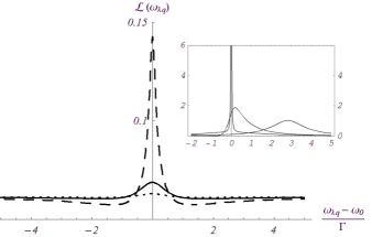
Figure 1: Unshifted luminescence ($\mathcal{L}$) for squeezing $\Lambda=0.9\Gamma$, bandwidth $B=50\Gamma$, and phonon dephasing $\gamma_{2}=0$ (dashed curve), $\gamma_{2}=3\Gamma$ (dotted curve), and $\gamma_{2}=\Gamma$ (solid curve). Insert: particle-hole lineshapes for different detuning $\delta_{k}=0,0.9\Gamma$ and $3\Gamma$ (from left to right). The curves are normalized to the total power.

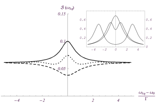
Figure 2: Squeezing spectra ($\mathcal{S}(\omega_{\lambda q})$) for squeezing $\Lambda=0.9\Gamma$, bandwidth $B=50\Gamma$, phonon dephasing of $\gamma_{2}=\Gamma$. It shows the in-phase quadrature fluctuations (solid curve) and out-of-phase quadrature fluctuations (dashed curve) for a fixed squeezing angle ($\alpha=0$). The linearly modulated squeezing phase spectrum is given for the in-phase quadrature (dotted curve). Insert: particle-hole squeezing spectra for different detuning $\delta_{k}=0,0.9\Gamma$ and $3\Gamma$ (from left to right) in the out-of-phase quadrature.

IV Realization

A possible realization of the above model is shown in Fig. (3) with the wave guide made of, e.g. metallic or Bragg mirrors .

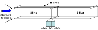
Figure 3: Schematic realization of the quantum well embedded in a wave guide cavity.

To minimize optical losses in the wave guide, which reduce the squeezing ($\Lambda$) of the light artoni-loudon ; schmidt ; patra , the interior of the wave guide should be filled with a material such as silica whose absorption is negligible. The reduction of squeezing due to losses is exponential artoni-loudon , with an exponent $-4\alpha l$, where $\alpha$ is the absorption coefficient, and $l$ is the distance. The length of the wave guide ($L$) should be much larger than the typical wavelength $\lambda=c/\omega_{0}$ to ensure that coupling transients in the vicinity of the opening do not reach the quantum well. Therefore $L$ should be of the order of $100-1000\mu m$ at least. The effect of dispersion is to rotate the squeezing phase blow-loudon , since pairs of correlated photon modes acquire a relative fixed phase over the distance in the dispersive material. This has no consequence for the power spectrum, but may result in a modulation of the squeezing phase with frequency, which can modify the squeezing spectrum, as was discussed above.

The central frequency $\omega_{0}$ should be above the cutoff frequency of the lowest wave guide mode. The range ($\omega_{0}\pm B/2$) should be tuned above the exciton ionization energy and below the optical phonon energy. The latter should make it possible to avoid the fast emission of optical phonons. The temperature should be small Levinson compared to $\sqrt{(\hbar\omega_{0}-E_{g})m^{*}s^{2}}$ ($s$ is the velocity of sound), so that spontaneous emission of acoustic phonons is the dominant electron-phonon scattering mechanism. The other important non-radiative source of dephasing is Coulomb scattering of the photo-excited electrons. This scattering rate is proportional to the density, and hence in our case to the bandwidth, for measurement times shorter than $\gamma_{1}^{-1}$.

We estimated the non-radiative rates for InAs esipov using the momentum relaxation time as an estimate for $\gamma_{2}$. In the quasi-elastic regime the momentum relaxation time is of the same order of the scattering rate Levinson . A simple Golden Rule calculation gives for a Boltzmann gas $\frac{1}{\tau_{e-e}}=\pi^{2}\frac{\hbar\epsilon_{B}}{m^{*}\epsilon}N$, where $N$ is surface density and $\epsilon_{B}=me^{4}/2\hbar^{2}$. For a zero lattice temperature and taking $\omega_{0}=E_{g}+20meV$, $\Gamma=1\mu eV$, $B=10\mu eV$ and density $2\times 10^{8}\,cm^{-2}$ we found this estimate to be $3.3\mu eV$ (i.e. $200ps$). These estimates are roughly supported experimentally Wang ; Haacke . In these experiments the dephasing times for the interband polarization were measured directly, and were shown to be of the order of $5ps$ for excitation density $N\sim 10^{10}\,\,\,cm^{-2}$, a density which is two order of magnitude higher than the one we consider ($N\sim 10^{8}\,\,\,cm^{-2}$). The dephasing times were also shown in one of the experiments Haacke to be much longer for the lower densities. The remaining dephasing in those densities was attributed to disorder, which we believe is a much weaker scattering process in the electron-hole plasma regime.

V Conclusions

To conclude, we found non-trivial lineshape structures in the spectra of a two mode squeezed vacuum scattered off a two band electronic system in two dimensions. They appear despite the flat spectrum of the incoming radiation and constant electronic density of states. These effects are due to the particular correlations of the squeezed vacuum and seem to be experimentally observable.

VI Acknowledgements

It is a pleasure to acknowledge valuable discussions with Y. B. Levinson and J. G. Groshaus. This work is supported by DIP Grant No. DIP-C7.1.

Appendix: The Polarization Fluctuation Equation

Here we derive the effective equations of motion which lead to the solution (10) for the fluctuations. We employ a consistent truncation of the hierarchy of equations of motion at the level of three and four-body correlations. We further assume the previous conditions $\Gamma\gg\gamma_{1}$. The e.o.m. for $\langle P^{\dagger}_{k}(t)P_{k^{\prime}}(t^{\prime})\rangle$ w.r.t. to one time argument is derived from the Hamiltonian $H=H_{0}+H_{I}$

$$\partial_{t}\langle P^{\dagger}_{k}(t)P_{k^{\prime}}(t^{\prime})\rangle=i\Delta\epsilon_{k}\langle P^{\dagger}_{k}(t)P_{k^{\prime}}(t^{\prime})\rangle+$$ (17)

$$+i\sum_{q}A^{*}_{q}\langle b^{\dagger}_{q}(t)\Delta n_{k}(t)P_{k^{\prime}}(t^{\prime})\rangle.$$

The derivative of $\langle b^{\dagger}_{q}(t)\Delta n_{k}(t)P_{k^{\prime}}(t^{\prime})\rangle$ is given by the two terms

$$\langle\dot{b^{\dagger}}_{q}(t)\Delta n_{k}(t)P_{k^{\prime}}(t^{\prime})\rangle=i\omega_{q}\langle b^{\dagger}_{q}(t)\Delta n_{k}(t)P_{k^{\prime}}(t^{\prime})\rangle+$$

$$+iA_{q}\sum_{k^{\prime\prime}}\langle P^{\dagger}_{k^{\prime\prime}}(t)\Delta n_{k}(t)P_{k^{\prime}}(t^{\prime})\rangle$$ (18)

$$\langle b^{\dagger}_{q}(t)\dot{\Delta n_{k}}(t)P_{k^{\prime}}(t^{\prime})\rangle=2i\sum_{q^{\prime}}A_{q^{\prime}}\langle b^{\dagger}_{q}(t)b_{q^{\prime}}(t)P^{\dagger}_{k}(t)P_{k^{\prime}}(t^{\prime})\rangle-$$

$$-2i\sum_{q^{\prime}}A^{*}_{q^{\prime}}\langle b^{\dagger}_{q}(t)b^{\dagger}_{q^{\prime}}(t)P_{k}(t)P_{k^{\prime}}(t^{\prime})\rangle.$$ (19)

We now assume that $\langle P^{\dagger}_{k^{\prime\prime}}(t)\Delta n_{k}(t)P_{k^{\prime}}(t^{\prime})\rangle\approx\langle P^{\dagger}_{k^{\prime\prime}}(t)P_{k^{\prime}}(t^{\prime})\rangle\langle\Delta n_{k}(t)\rangle$ is very small, since in the steady state $\langle\Delta n_{k}(t)\rangle\ll 1$ (note that the correlation $\langle P^{\dagger}_{k^{\prime\prime}}(t)\Delta n_{k}(t)P_{k^{\prime}}(t^{\prime})\rangle$ cannot decouple to contributions with an average polarization $\langle P^{\dagger}_{k}\rangle$). Next we assume that at the second order in the system-reservoir interaction $A_{q}$, the correlations can be decoupled by approximating for the total density matrix $\rho_{tot}=\rho_{sys}\otimes\rho_{res}$. As a result we get for the correlations in the r.h.s. of Eq. (Appendix: The Polarization Fluctuation Equation)

$$\langle b^{\dagger}_{q}(t)b_{q^{\prime}}(t)P^{\dagger}_{k}(t)P_{k^{\prime}}(t^{\prime})\rangle\approx\langle b^{\dagger}_{q}(t)b_{q^{\prime}}(t)\rangle\langle P^{\dagger}_{k}(t)P_{k^{\prime}}(t^{\prime})\rangle$$

$$\langle b^{\dagger}_{q}(t)b^{\dagger}_{q^{\prime}}(t)P_{k}(t)P_{k^{\prime}}(t^{\prime})\rangle\approx\langle b^{\dagger}_{q}(t)b^{\dagger}_{q^{\prime}}(t)\rangle\langle P_{k}(t)P_{k^{\prime}}(t^{\prime})\rangle.$$

Substituting all the contributions in (Appendix: The Polarization Fluctuation Equation) back into (17) we have for $\langle P^{\dagger}_{k}(t)P_{k^{\prime}}(t^{\prime})\rangle$

$$\partial_{t}\langle P^{\dagger}_{k}(t)P_{k^{\prime}}(t^{\prime})\rangle=i\Delta\epsilon_{k}\langle P^{\dagger}_{k}(t)P_{k^{\prime}}(t^{\prime})\rangle-2\sum_{qq^{\prime}}A_{q}^{*}A_{q^{\prime}}e^{i\omega_{q}t}\int^{t}dt^{\prime\prime}e^{-i\omega_{q}t^{\prime\prime}}\langle b^{\dagger}_{q}(t^{\prime\prime})b_{q^{\prime}}(t^{\prime\prime})\rangle\langle P^{\dagger}_{k}(t^{\prime\prime})P_{k^{\prime}}(t^{\prime})\rangle+$$ (20)

$$+2\sum_{qq^{\prime}}A_{q}^{*}A_{q^{\prime}}^{*}e^{i\omega_{q}t}\int^{t}dt^{\prime\prime}e^{-i\omega_{q}t^{\prime\prime}}\langle b^{\dagger}_{q}(t^{\prime\prime})b^{\dagger}_{q^{\prime}}(t^{\prime\prime})\rangle\langle P_{k}(t^{\prime\prime})P_{k^{\prime}}(t^{\prime})\rangle.$$

Similarly, the equation for the correlation $\langle P_{k}(t)P_{k^{\prime}}(t^{\prime})\rangle$ is given by

$$\partial_{t}\langle P_{k}(t)P_{k^{\prime}}(t^{\prime})\rangle=-i\Delta\epsilon_{k}\langle P_{k}(t)P_{k^{\prime}}(t^{\prime})\rangle-2\sum_{qq^{\prime}}A_{q}A_{q^{\prime}}^{*}e^{-i\omega_{q}t}\int^{t}dt^{\prime\prime}e^{i\omega_{q}t^{\prime\prime}}\langle b^{\dagger}_{q}(t^{\prime\prime})b_{q^{\prime}}(t^{\prime\prime})\rangle\langle P^{\dagger}_{k}(t^{\prime\prime})P_{k^{\prime}}(t^{\prime})\rangle+$$ (21)

$$+2\sum_{qq^{\prime}}A_{q}A_{q^{\prime}}e^{-i\omega_{q}t}\int^{t}dt^{\prime\prime}e^{i\omega_{q}t^{\prime\prime}}\langle b_{q}(t^{\prime\prime})b_{q^{\prime}}(t^{\prime\prime})\rangle\langle P_{k}(t^{\prime\prime})P_{k^{\prime}}(t^{\prime})\rangle.$$

We now employ the correlations (4) and the Markov approximation to obtain

$$\partial_{t}\langle P^{\dagger}_{k}(t)P_{k^{\prime}}(t^{\prime})\rangle=(i\Delta\epsilon_{k}-\Gamma(\Delta\epsilon_{k}))\langle P^{\dagger}_{k}(t)P_{k^{\prime}}(t^{\prime})\rangle+\Lambda(\Delta\epsilon_{k})e^{2i\delta_{k}t}\langle P_{k}(t)P_{k^{\prime}}(t^{\prime})\rangle$$ (22)

$$\partial_{t}\langle P_{k}(t)P_{k^{\prime}}(t^{\prime})\rangle=(-i\Delta\epsilon_{k}-\Gamma(\Delta\epsilon_{k}))\langle P_{k}(t)P_{k^{\prime}}(t^{\prime})\rangle+\Lambda^{*}(\Delta\epsilon_{k})e^{-2i\delta_{k}t}\langle P^{\dagger}_{k}(t)P_{k^{\prime}}(t^{\prime})\rangle.$$

References

• (1) D. Kleppner, Phys. Rev. Lett. 47, 233 (1981).
• (2) P. Goy, J. M. Raimond, M. Gross and S. Haroche, Phys. Rev. Lett. 50, 1903 (1983).
• (3) C. W. Gardiner, Phys. Rev. Lett. 56 (18), 1917 (1986).
• (4) G. M. Palma and P. L. Knight, Phys. Rev. A 39 (4), 1962 (1989).
• (5) H. J. Charmichael, A. S. Lane, D. F. Walls, J. Mod. Opt. 34 (6/7), 821 (1987).
• (6) G. S. Solomon, M. Pelton, Y. Yamamoto, Phys. Rev. Lett. 86, 3903 (2001).
• (7) C. W. Gardiner, A. S. Parkins, M. J. Collet, J. Opt. Soc. Am. B, 4 (10), 1683 (1987).
• (8) S. D. Brorson, H. Yokoyama and E. P. Ippen, IEEE J. Quantum Electron. 26 (9), 1492 (1990).
• (9) E. Ginossar and S. Levit, unpublished.
• (10) G. Khitrova, H. M. Gibbs, F. Jahnke, M. Kira and S. W. Koch, Rev. Mod. Phys. 71, 1591 (1999).
• (11) H. Haug and S. W. Koch, Quantum Theory of the Optical and Electronic Properties of Semiconductors, World-Scientific (1990).
• (12) M. Lindberg and S. W. Koch, Phys. Rev. B 38 (5), 3342 (1988).
• (13) M. Kira, W. Hoyer, S. W. Koch, Solid State Comm. 129, 733 (2004).
• (14) S. Chatterjee et. al., Phys. Rev. Lett. 92 (6), 067402 (2004).
• (15) M. Artoni and R. Loudon, Phys. Rev. A, 59 (3), 2279 (1999).
• (16) K. J. Blow, R. Loudon, S. J. D. Phoenix and T. J. Shepherd, Phys. Rev. A, 42(7), 4102 (1990).
• (17) E. Schmidt, L. Knöll, and D. G. Welsch, Phys. Rev. A, 54 (1), 843 (1996).
• (18) M. Patra and C. W. J. Beenakker, Phys. Rev. A, 61, 063805 (2000).
• (19) V. F. Gantmakher and Y. B. Levinson, Carrier scattering in metals and semiconductors, Elseviers Science Publishers (1987), Chap. 4.
• (20) S. E. Esipov, Y. B. Levinson, Advances in Physics, 36 (3), 331 (1987).
• (21) Hailin Wang, Jagdeep Shah and T. C. Damen, Phys. Rev. Lett. 74 (15), 3065 (1995).
• (22) S. Haacke, R. A. Taylor, R. Zimmermann, I. Bar-Joseph and B. Deveaud, Phys. Rev. Lett. 78 (11), 2228 (1997).
• (23) H. J. Carmichael, Statistical methods in quantum optics, Springer (1999).