Investment strategy due to the minimization of portfolio noise level by observations of coarse-grained entropy

Abstract

Using a recently developed method of noise level estimation that makes use of properties of the coarse grained-entropy we have analyzed the noise level for the Dow Jones index and a few stocks from the New York Stock Exchange. We have found that the noise level ranges from $40$ to $80$ percent of the signal variance. The condition of a minimal noise level has been applied to construct optimal portfolios from selected shares. We show that implementation of a corresponding threshold investment strategy leads to positive returns for historical data.

1 Introduction

Although it is a common believe that the stock market behaviour is driven by stochastic processes [1, 2, 3] it is difficult to separate stochastic and deterministic components of market dynamics. In fact the deterministic fraction follows usually from nonlinear effects and can possess a non-periodic or even chaotic characteristic [4, 5]. The aim of this paper is to study the level of determinism in time series coming from stock market. We will show that our noise level analysis can be useful for portfolio optimization.

We employ here a method of noise-level estimation that has been described in details in [6]. The method is quite universal and it is valid even for high noise levels. It makes use of the functional dependence of coarse-grained correlation entropy $K_{2}(\varepsilon)$ [7] on the threshold parameter $\varepsilon$. Since the function $K_{2}(\varepsilon)$ depends in a characteristic way on the noise standard deviation $\sigma$ thus one can estimate the noise level $\sigma$ observing the dependence $K_{2}(\varepsilon)$. The validity of our method has been verified by applying it for the noise level estimation in several chaotic models [7] and for the Chua electronic circuit contaminated by noise. The method distinguishes a noise appearing due to the presence of a stochastic process from a non-periodic deterministic behaviour (including the deterministic chaos). Analytic calculations justifying our method have been developed for the gaussian noise added to the observed deterministic variable. It has been also checked in numerical experiments that the method works properly for a uniform noise distribution and at least for some models with dynamical noise corresponding to the Langevine equation [6].

2 Calculations of noise level in stock market data

We define the noise level as the ratio of standard deviation of noise $\sigma$ to the standard deviation of data $\sigma_{data}$

$$NTS=\frac{\sigma}{\sigma_{data}}$$ (1)

Using this definition and our noise level estimation method [6] we have analyzed the noise level in data recorded at the New York Stock Exchange (NYSE). Let us consider logarithmic daily returns for the Dow Jones Industrial Average (DJIA)

$$x_{i}=\ln\left(\frac{P_{i}}{P_{i-1}}\right).$$ (2)

Fig. 1 presents the plot of the noise level $NTS$ for a corresponding time series $x_{i}$ where values of $NTS$ have been calculated as a function of a trading day. The noise level has been determined in windows of the length $3000$ days and is pointed in the middle of every window. As one can see the level of noise ranges from $60\%$ to $90\%$ what makes any point to point forecasting impossible. We should mention that since the relative noise variance is $NTS^{2}$, thus in our case the noise variance is $40-80\%$ of the data variance. It follows that there are time periods when the percent of an unknown deterministic part approaches the level $60\%$ of the signal.

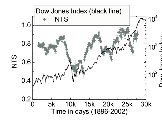
Figure 1: The noise level $NTS$ calculated for Dow Jones index (1896-2002).

Similar estimations of the noise level have been performed for selected stocks of the NYSE. Results for the mean values of corresponding NTS parameters are presented in the Table 1. As one can expect the noise level of a single stock is much larger than for the DJIA. This is because deterministic parts of different stock prices are usually positive correlated what is less common for stochastic components.

The crucial point for our investment strategy are correlations between a temporary value of noise level and a temporary value of price changes. We have found that for the majority of considered stocks the correlation coefficient $\rho$ is much larger than zero (see the Table 1) in the time period when trends of these stock were negative. A negative correlation coefficient has been observed for one share with a positive share. Following these observations we have formed the following heuristic rule: temporary price changes are mostly consistent with the trend for a small noise level but they are frequently opposed to the trend for a large noise level (the noise level should be measured locally). One can say that when price changes are more stochastic investors are more disoriented than for a more deterministic price motion and they more frequently trade against the general trend.

Table 1: Stocks recorded at the NYSE for the period 01.01.1999-31.12.2000. Table of the values of the noise levels $NTS$, correlation coefficient $\rho$ between prices changes and the noise levels and returns in the studied period.

Stock	$NTS$	$\rho$	returns at the period
Apple (Ap)	$77\%$	$0.53$	$-63\%$
Bank of America (Boa)	$93\%$	$0.22$	$-24\%$
Boeing (Bg)	$94\%$	$-0.45$	$98\%$
Cisco (Ci)	$85\%$	$0.57$	$-59\%$
Compaq (Cq)	$93\%$	$-0.09$	$-66\%$
Ford (Fo)	$91\%$	$-0.16$	$-60\%$
General Electric (Ge)	$86\%$	$0.75$	$-53\%$
General Motors (Gm)	$91\%$	$0.44$	$-28\%$
Ibm (Ibm)	$75\%$	$0.023$	$-55\%$
Mcdonald (Md)	$93\%$	$0.2$	$-57\%$
Texas Instrument (Te)	$76\%$	$0.77$	$-45\%$

3 Investment strategy

Using the fact that the level of noise is correlated with the stock price changes, one can create a portfolio which can maximize the profit. In the first step we construct a portfolio with the minimal value of the stochastic variable. We assume that one can do this by maximization of the following quantity:

$$\mathcal{B}=\sum\limits_{i=1}^{M}\sum\limits_{j=1}^{M}p_{i}p_{j}\frac{\sigma_{i,D}}{\sigma_{i}}\frac{\sigma_{j,D}}{\sigma_{j}}\rho_{i,j}=max.$$ (3)

where $\sigma_{i,D}$ is a standard deviation of deterministic part of the stock $i$, $\sigma_{i}$ is the standard deviation of the noise in this stock and $\rho_{i,j}$ is the correlation between deterministic parts of stocks $i$ and $j$. The maximal value of $\mathcal{B}$ can be performed with the help of the steepest descent method by changing the variables $p_{i}$ and keeping the normalization constraint $\sum_{i=1}^{M}p_{i}=1$.

Now let us define our investment strategy as follows: if the past trend of portfolio is positive $m_{p}>0$ and the noise level is small ($NTS_{p}<NTS_{treshhold}$) we invest in the calculated portfolio. We invest also in the portfolio when it is more stochastic ($NTS_{p}>NTS_{treshhold}$) but its trend is negative $m_{p}<0$. We invest against the portfolio in the remaining two cases.

Table 2 presents the values $P_{p}$ for a few portfolios at the end of a trading period when the above investment strategy has been used. The results are compared to mean values of the prices of stocks $P_{m}$ at the same moment and a relative profit of our investment strategy is shown: $(P_{p}/P_{m}-1)\cdot 100\%$. To get the proper normalization we set the values $P_{p}$ and $P_{m}$ to one at the beginning of the trading period. Although the above analysis gives very promising results one should mention that all commissions costs have been omitted and what is more crucial we have assumed an unlimited possibility of short-sellings. As result our portfolios are very risky. When one limits the possible short-selling level the risk and returns are lower.

In the Table 3 the results are summarized for several studied portfolios. We have found that $62\%$ of portfolios had positive returns even that for the considered time period almost all single stock returns were negative (see Table 1).

Table 2: The value of optimized portfolio $P_{p}$ at the end of studied period (01.01.1999-31.12.2000) in comparison to behavior of mean prices $P_{m}$.

Stocks	$P_{m}$	$P_{p}$	$(P_{p}/P_{m}-1)\cdot 100\%$
Ap, Bg, Cq, Ge, Ibm, Md, Boa, Ci	$0.58$	$3.41$	$487\%$
Ap, Boa, Bg, Ci, Cq, Fo, Ge, Gm	$0.56$	$6.65$	$1087\%$
Bg, Ci, Cq, Fo, Ge, Gm, Ibm, Te	$0.60$	$1.01$	$68\%$
Boa, Bg, Ci, Cq, Fo, Ge, Gm, Ibm	$0.64$	$0.48$	$-25\%$
Ci, Cq, Fo, Ge, Gm, Ibm, Te, Md	$0.55$	$1.86$	$238\%$
Md, Ibm, Cq, Te, Boa, Fo, Ap, Ge	$0.48$	$8.08$	$1583\%$
all studied stocks	$0.56$	$8.45$	$1408\%$

Table 3: Summary of the portfolio optimization. Analysis was done for the period 01.01.1999-31.12.2000.

No of elaborated portfolios	$55$
Portfolios with negative returns	$38\%$
Portfolios with positive returns	$62\%$
Portfolios with returns smaller than mean	$29\%$
Portfolios with returns larger than mean	$71\%$

4 Conclusions

In conclusion we have found that the deterministic part of stock market data at NYSE is in the range $20-60\%$ of the data variance. The estimation of noise level can be useful for portfolio optimization. The resulting investment strategy gives in average positive returns.

5 Acknowledgement

This work has been partially supported by the KBN Grant 2 P03B 032 24 (KU) and by a special Grant Dynamics of Complex Systems of the Warsaw University of Technology (JAH).

References

- [1] J.Voit, The Statistical Mechanics of Financial Markets, (Springer-Verlag 2001).
- [2] J.P. Bouchaud, M. Potters, Theory of financial risks - from statistical physics to risk management, (Cambridge University Press 2000).
- [3] R.N. Mantegna, H.E. Stanley, An Introduction to Econophysics. Correlations and Complexity in Finance, (Cambridge University Press 2000).
- [4] E.E. Peters, Chaos and Order in the Capital Markets. A new view of cycle, Price, and Market Volatility, (John Wiley Sons 1997).
- [5] J.A. Hołyst, M. Żebrowska i K. Urbanowicz, European Physical Journal B 20, 531-535 (2001).
- [6] K. Urbanowicz and J. A. Hołyst, Phys. Rev. E 67, 046218 (2003).
- [7] H. Kantz and T. Schreiber, Nonlinear Time Series Analysis (Cambridge University Press, Cambridge, 1997).