Theory of fluctuations in a two-band superconductor

Abstract

A theory of fluctuations in two-band superconductor MgB₂ is developed. Since the standard Ginzburg-Landau (GL) approach fails in description of its properties, we generalize it basing on the microscopic theory of a two-band superconductor. Calculating the microscopic fluctuation propagator, we build up the nonlocal two-band GL functional and the corresponding time-dependent GL equations. This allows us to calculate the main fluctuation observables such as fluctuation specific heat and conductivity.

I Introduction

The celebrated phenomenological Ginzburg-Landau (GL) theory of superconductivity was introduced in the seminal paper by Ginzburg and Landau GL50 and has been proving ever since to be one of most fruitful and universal tools in the description basic properties of superconductors. The examples of its success range from the prediction of the Abrikosov vortex state AbrikosovJETP57 to the recent advance in understanding the complex vortex phase diagram of the high-temperature superconductors BGFLV94 and the properties of mesoscopic superconducting systems F03 . The Gor’kov’s derivation of the GL equations from the BCS theory G58 that have put the GL theory on a firm microscopic basis and related phenomenological constants to material parameters, completed the construction of the GL theory of superconductors.

The GL theory describes well the properties of almost all superconductors near transition temperature and is successful even when dealing with the superconductors with quite complicated band structures. The notorious exception from the rule is recently discovered multiband superconductor magnesium diboride (MgB₂). As it was shown GK03a ; GK03b , the GL theory applies to MgB₂ only in the very immediate vicinity of the transition temperature, $T_{c}$, i.e. within the interval which turns out to be much more narrow than the usual one given by the condition $|T-T_{c}|\ll T_{c}$. The origin of this narrowing of the interval of validity lies in the sophisticated band structure of the material and reflects the specific interplay between its single-electron and superconducting characteristics. Namely, the Brillouin zone of MgB₂ consists of the two families of bands: the quasi-two-dimensional $\sigma$-bands with the strong superconductivity and the weakly superconducting three-dimensional $\pi$-bands. Due to the large difference in anisotropy, the c-axis coherence length of the $\pi$-bands, $\xi_{2,z}$, is much larger than the c-axis coherence length of the $\sigma$-bands, $\xi_{1,z}$. Formation of the global coherent superconductivity with the unique order parameter implies the appearance of the associated unique effective coherence length $\widetilde{\xi}_{z}\left(T\right)$, which turns out to be much smaller than $\xi_{2,z}$ at almost any temperature. As a consequence, the GL applicability interval shrinks to the parametrically narrow range of temperatures where $\widetilde{\xi}_{z}\left(T\right)\gg\xi_{2,z}$. Beyond this temperature range the system is strongly nonlocal along the $z$-axis; to describe such a nonlocality one has to employ a generalized nonlocal GL model GK03b . One of the spectacular manifestations of the non-GL behavior in MgB₂ is the strong temperature dependence of the $H_{c2}$ anisotropy close to $T_{c}$ hc2anisotropy .

The description of superconducting fluctuations is one of the major fields for the application of the GL theory. Since the standard GL approach turns out to be insufficient for MgB₂, a generalization of the GL theory is required in order to describe its fluctuation properties. The variation of the order parameter on the scales smaller than the largest intrinsic coherence length means that the usually assumed local approximation does not hold anymore and the corresponding short-wavelength fluctuations have to be taken into account.

In the present paper we develop a nonlocal theory of superconducting fluctuations that applies to a strongly anisotropic two-band superconductor Multi-Two and show that the short-wavelength fluctuations are essential in it near the critical temperature. We start with the derivation of the microscopic fluctuation propagator for a such two-band model. Then we use it to nonlocal two-band GL functional and the corresponding time-dependent GL (TDGL) equations. This, in particular, allows us to calculate the kinetic and thermodynamic observable quantities including the fluctuational specific heat and conductivity.

As we have already stated, the main source of the non-GL behavior is the nonlocality in the $c$ direction, i.e., the strong wave-vector dependence of c-axis coherence length. The conventional local form of the GL equations turns out to be valid only within the narrow interval of temperatures, $|T-T_{c}|/T_{c}\ll\xi_{1,z}^{2}/\xi_{2,z}^{2}+S_{12}\ll 1$, where $S_{12}\ll 1$ is the relative interband interaction constant which will be specified below. Beyond this interval, the superconducting correlations in the $\pi$-band become nonlocal and their contribution to the effective coherence length rapidly decreases. Far away from $T_{c}$ the effective c-axis coherence length is determined only by the $\sigma$-band. In other words, the effective c-axis coherence diverges for $T\rightarrow T_{c}$ faster than it could be expected from the naive GL extrapolation, $\widetilde{\xi}_{z}(T)\propto 1/\sqrt{T-T_{c}}$, started from high temperatures. This also leads to the decrease of the effective anisotropy factor $\Gamma(T)=\widetilde{\xi}_{x}(T)/\widetilde{\xi}_{z}(T)$. As a consequence, the temperatures dependencies of all fluctuation corrections exhibit the characteristic crossovers between the dominating $\sigma$-band regime (far away from $T_{c}$) and the “true” GL regime (very close to $T_{c}$). For example, the $c$-axis component of the paraconductivity diverges faster in the immediate vicinity of $T_{c}$ than one could expect from high-temperature extrapolation using the Aslamazov-Larkin formula LV02 while the fluctuation specific heat and $ab$ component of the paraconductivity diverge slower than the corresponding extrapolations. We will obtain the temperature dependencies of these fluctuation corrections.

II Critical temperature and fluctuation propagator

II.1 Cooper pairing in two-band model

The BCS theory was generalized to the case of the two-band electron spectrum long time ago Suhl ; Moskal and has been extended recently to include the specific features of magnesium diboride in Refs. Kortus, ; An, ; LiuPRL01, ; Kong, ; Yildirim, ; Choi, . We briefly overview this theory rewriting it in terms of Green’s function formalism. The two-band BCS Hamiltonian is given by

$$\mathcal{H}=\sum_{\mathbf{p},\alpha,\sigma}\zeta_{\alpha}\left(\mathbf{p}\right)\psi_{\alpha,\mathbf{p},\sigma}^{{\dagger}}\psi_{\alpha,\mathbf{p},\sigma}-\sum_{\mathbf{p,p}^{\prime},\mathbf{q},\alpha,\beta,\sigma,\sigma^{\prime}}g_{\alpha\beta}\psi_{\alpha,\mathbf{p+q,}\sigma}^{{\dagger}}\psi_{\alpha,-\mathbf{p},-\sigma}^{{\dagger}}\psi_{\beta,-\mathbf{p}^{\prime},-\sigma^{\prime}}\psi_{\beta,\mathbf{p}^{\prime}+\mathbf{q,}\sigma^{\prime}},$$ (1)

where $\psi_{\alpha,\mathbf{p},\sigma}^{{\dagger}}$ and $\psi_{\alpha,\mathbf{p},\sigma}$ are the creation and annihilation field operators in the Heisenberg representation for quasiparticle in band $\alpha$ with momentum $\mathbf{p}$ and spin $\sigma$,

$$\zeta_{\alpha}\left(\mathbf{p}\right)=\mathbf{v}_{\alpha}\left(\mathbf{p}-\mathbf{p}_{F\alpha}\right)$$ (2)

is the quasiparticle spectrum, $\mathbf{v}_{\alpha}$, $\mathbf{p}_{F\alpha}$ are the Fermi velocity and momentum of the $\alpha$-band. The matrix nature of the electron-electron interaction $-g_{\alpha\beta}$ in (1) reflects the possibility of the interband interactions. The free electron Green’s functions for each band have the usual form $G_{\alpha}\left(r,r^{\prime},\tau,\tau^{\prime}\right)=-i\left\langle T_{\tau}\psi_{\alpha}\psi_{\alpha}^{\prime{\dagger}}\right\rangle$, where $T_{\tau}$ is the time-ordering operator. In the Matsubara representation,

$$G_{\alpha}\left(\mathbf{p},\varepsilon_{n}\right)=\left(i\varepsilon_{n}-\zeta_{\alpha}\left(\mathbf{p}\right)\right)^{-1}$$ (3)

with $\varepsilon_{n}=2\pi T(n+1/2)$ being the fermionic Matsubara frequencies.

Now we turn to calculation of the fluctuation propagator $L_{\alpha\beta}$ which characterizes the properties of fluctuation Cooper pairs and their effect on observable quantities of superconductor above $T_{c}$.LV02 Note first of all, that the interband electron interactions do not result in the Cooper pairing of the electrons from different bands but rather lead to the transfer of the pairing correlations between the bands. Indeed, the Cooper pairing means the appearance of superconducting-type correlations between two similar states obeying the condition of the time reversal symmetry. This means that pairing is possible only for electrons belonging to the same band, otherwise the electron states are too diverse (in terms of the plane waves description, their momenta are not the opposite) and the integral of the product of their wave functions is zero. Thus the formation of unique condensate should be understood as the result of the intraband electron correlations and subsequent “travel”of the Cooper pair from one band to another due to off-diagonal interaction components $g_{12}$ and $g_{21}$. Hence, in terms of diagrams, the entrance and exit lines of the fluctuation propagator must belong to the same bands (see Fig. 1) and it can be presented as the $2\times 2$ matrix $L_{\alpha\beta}\left(\mathbf{q},\Omega_{k}\right)$ where $\Omega_{k}\!=2\pi Tk$ are the bosonic Matsubara frequencies. The corresponding Dyson equation for fluctuation propagator can be written in the ladder approximation as (see Fig. 1)

$$L_{\alpha\beta}=-g_{\alpha\beta}+g_{\alpha\gamma}\Pi_{\gamma\delta}L_{\delta\beta},$$ (4)

where $\Pi_{\alpha\beta}\left(\mathbf{q},\Omega_{k}\right)$ is the matrix polarization operator which is determined by two Green’s functions loop LV02 . Without interband electron scattering the only nonzero components of the operator $L_{\alpha\beta}$ are the diagonal ones.

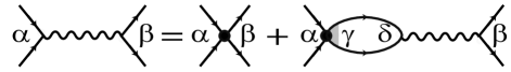
Figure 1: Graphic representation of Dyson equation (4) for the fluctuation propagator $L_{\alpha\beta}$ (wavy line). The Greek letters indicate the band indices. The black dot represents the coupling-constants matrix $-g_{\alpha\beta}$, the loop represents the polarization operator $\Pi_{\gamma\delta}$, and the shaded triangle represents the scattering vertex $C_{\gamma\gamma}$.

Turning to the role of electron scattering, let us note that at the first sight the short-range impurity potential might lead to the scattering of electrons all over the whole Fermi surface which would result in the equalization of all gap values and reduction of $T_{c}$. However, it is well established now that this does not happen in MgB₂: even in the samples with rather strong intraband scattering, interband scattering remains rather weak. This property gave possibility to fabricate samples with very high upper critical fields (up to 50 tesla) which have transition temperatures only slightly smaller than clean materialhighHc2 . Weakness of the interband scattering has been explained by Mazin et al. in Ref. M03, who argued that different parity symmetry of the $\sigma$- and $\pi$- orbitals leads to strong reduction of the impurity scattering matrix element between these bands. For simplicity, we will completely neglect the interband scattering. In this case the off-diagonal components of the polarization operator vanish. The averaging over impurities position will result just in the usual renormalization of the Green’s functions: $\varepsilon_{n}\rightarrow\varepsilon_{n}+1/2\tau_{\alpha}$ ($\tau_{\alpha}$ is the corresponding intraband scattering time) and to the appearance of the scattering vertex part $C_{\alpha\alpha}$ in the expression for the polarization operator

$$\Pi_{\alpha\alpha}\left(\mathbf{q},\Omega_{k}\right)=T\sum_{\varepsilon_{n}}\int\frac{d\mathbf{p}}{\left(2\pi\right)^{3}}C_{\alpha\alpha}(\mathbf{q},\varepsilon_{n+k},-\varepsilon_{n})G_{\alpha}\left(\mathbf{p+q},\varepsilon_{n}+\Omega_{k}\right)G_{\alpha}\left(-\mathbf{p},-\varepsilon_{n}\right).$$ (5)

The scattering vertex part can be calculated in the ladder approximationAGD . In the case of a dirty metal $\left(T\tau_{\alpha\alpha}\ll 1\right)$ this givesLV02

$$C_{\alpha\alpha}(\mathbf{q},\varepsilon_{n+k},-\varepsilon_{n})\!=\!\frac{1/\tau_{\alpha\alpha}}{|\varepsilon_{n}\!+\!\varepsilon_{n+k}|\!+\!\hat{D}_{\alpha}q^{2}}\theta\left(\varepsilon_{n+k}\varepsilon_{n}\right),$$ (6)

leading to the following result for the polarization operator

$$\Pi_{\alpha\alpha}(\mathbf{q},\Omega_{k})\!=\!\nu_{\alpha}\!\left[\ln\!\frac{\omega_{D}}{2\pi T}\!-\!\psi\!\left(\frac{1}{2}\!+\!\frac{|\Omega_{k}|\!+\!\hat{D}_{\alpha}q^{2}}{4\pi T}\right)\right],$$ (7)

where $\nu_{\alpha}$ is the density of states in the band $\alpha$, $\omega_{D}$ is the Debye frequency and $\psi\left(x\right)$ is the digamma-function. We introduced above the notation for the diffusion-coefficient tensor acting in the momentum and band spaces:

$$\hat{D}_{\alpha}q^{2}\equiv\sum_{a}D_{\alpha,a}q_{a}^{2}.$$ (8)

The diffusivities $D_{\alpha,a}$ determine the band coherence lengths as $\xi_{\alpha,a}^{2}=\pi D_{\alpha,a}/8T$. For magnesium diboride the ratio

$$r=D_{2,z}/D_{1,z}=\xi_{2,z}^{2}/\xi_{1,z}^{2},$$ (9)

is large, $r\gg 1$, due to the large difference between the band Fermi velocities in the $c$ direction Kortus ; An . This parameter will play an important role in the following consideration.

The inversion of the Dyson equation (4) gives

$$\widehat{L}^{-1}=-\widehat{\emph{g}}^{-1}+\widehat{\Pi}.$$ (10)

We will use now this general expression to reconsider the main properties of two-band superconductivity and to describe the corresponding fluctuation properties.

II.2 Critical temperature

The critical temperature of a two-band superconductor is determined by the condition $\det\widehat{L}^{-1}=0$ taken at $\Omega_{k}=0$ and $\mathbf{q}=0$:

$$\left(\frac{g_{22}}{\det\widehat{\emph{g}}}\!-\!\nu_{1}\ln\frac{2\gamma_{E}\omega_{D}}{\pi T_{c}}\right)\!\!\left(\frac{g_{11}}{\det\widehat{\emph{g}}}\!-\!\nu_{2}\ln\frac{2\gamma_{E}\omega_{D}}{\pi T_{c}}\right)\!-\!\frac{g_{21}g_{12}}{\det^{2}\widehat{\emph{g}}}\!=\!0.$$

with $\ln\gamma_{E}\equiv C_{E}\approx 0.577$ being the Euler constant. Introducing the coupling-constants matrix as

$$\widehat{\lambda}=\left(\begin{array}[c]{cc}\nu_{1}g_{11}&\nu_{2}g_{12}\\ \nu_{1}g_{21}&\nu_{2}g_{22}\end{array}\right),$$

we can find that the transition temperature is determined by its largest eigenvalue,

$$\tilde{\lambda}=\frac{\lambda_{+}}{2}+\sqrt{\frac{\lambda_{-}^{2}}{4}+\lambda_{12}\lambda_{21}}$$

with $\lambda_{\pm}\equiv\lambda_{11}\pm\lambda_{22}$, and it is given by the BCS-type equation:

$$\ln\frac{2\gamma_{E}\omega_{D}}{\pi T_{c}}=\tilde{\lambda}^{-1}.$$

Following Ref. GK03b, , we introduce the inverse coupling-constants matrix

$$\widehat{W}=\left(\begin{array}[c]{cc}W_{11}&-W_{12}\\ -W_{21}&W_{22}\end{array}\right)\equiv\widehat{\lambda}^{-1}-\tilde{\lambda}^{-1}\hat{I}=\frac{1}{\det\widehat{\lambda}}\left(\begin{array}[c]{cc}\!\sqrt{\lambda_{-}^{2}/4\!+\!\lambda_{12}\lambda_{21}}\!-\!\lambda_{-}/2&-\lambda_{21}\\ -\lambda_{12}&\!\sqrt{\lambda_{-}^{2}/4\!+\!\lambda_{12}\lambda_{21}}\!+\!\lambda_{-}/2\end{array}\right),$$

where $\hat{I}$ is the unit matrix and $\det\widehat{\lambda}\equiv\lambda_{11}\lambda_{22}-\lambda_{12}\lambda_{21}$. From the definition of the matrix $\widehat{W}$ is evident that it is degenerate, $\det\widehat{W}\equiv W_{11}W_{22}-W_{12}W_{21}=0.$ Having in mind applications of our theory to MgB₂, we will use the numerically computed effective coupling constants for this compound Golub :

$$\left(\begin{array}[c]{cc}W_{11}&W_{12}\\ W_{21}&W_{22}\end{array}\right)=\left(\begin{array}[c]{cc}0.088&0.535\\ 0.424&2.56\end{array}\right).$$ (11)

We see now that apart from the already mentioned large ratio $r$ (9), another characteristic small parameter, the relative interband coupling,

$$S_{12}=\frac{W_{11}}{W_{22}}\approx 0.035\ll 1$$ (12)

appearsGK03a ; GK03b . In what follows we will demonstrate that it is the interplay between these two parameters that defines the rich picture of  fluctuations that occurs beyond the traditional GL theory.

II.3 Fluctuation propagator

In terms of the notations introduced above, the inverse matrix for the propagator (10) assumes the form

$$\widehat{L}^{-1}(\Omega_{k},\mathbf{q})=-\left(\begin{array}[c]{cc}W_{11}+\epsilon+\beta_{1}\left(|\Omega_{k}|,q\right)&-W_{12}\\ -W_{21}&W_{22}+\epsilon+\beta_{2}\left(|\Omega_{k}|,q\right)\end{array}\right)\left(\begin{array}[c]{cc}\nu_{1}&0\\ 0&\nu_{2}\end{array}\right),$$ (13)

where $\epsilon=\ln(T/T_{c})$,

$$\beta_{\alpha}\left(\omega,q\right)\equiv\beta\left[\frac{\pi}{8T}(\omega+\hat{D}_{\alpha}q^{2})\right],$$

and

$$\beta(x)\equiv\psi\left(1/2+2x/\pi^{2}\right)-\psi\left(1/2\right)=\left\{\begin{tabular}[c]{l}$x,\ \ x\ll 1$\\ $\ln x+C_{E}+\ln(8/\pi^{2}),\ x\gg 1$\end{tabular}\right.,$$ (14)

Note that due to the identity $W_{12}\nu_{2}=W_{21}\nu_{1}$, the matrix $\widehat{L}^{-1}(\Omega_{k},\mathbf{q})$ is symmetric.

Calculating $\det\widehat{L}^{-1}$ and inverting the matrix, one can present $\widehat{L}(\Omega_{k},\mathbf{q})$ as

$$\widehat{L}(\Omega_{k},\mathbf{q})=\frac{\left(\begin{array}[c]{cc}\widetilde{W}_{22}+\widetilde{\theta}\left[\epsilon+\beta_{2}\left(|\Omega_{k}|,q\right)\right]&\widetilde{W}_{21}\\ \widetilde{W}_{12}&\widetilde{W}_{11}+\widetilde{\theta}\left[\epsilon+\beta_{1}\left(|\Omega_{k}|,q\right)\right]\end{array}\right)\left(\begin{array}[c]{cc}\nu_{1}^{-1}&0\\ 0&\nu_{2}^{-1}\end{array}\right)}{\epsilon+\left[\widetilde{W}_{11}+\widetilde{\theta}\epsilon\right]\beta_{2}\left(|\Omega_{k}|,q\right)+\left[\widetilde{W}_{22}+\widetilde{\theta}\beta_{2}\left(|\Omega_{k}|,q\right)\right]\beta_{1}\left(|\Omega_{k}|,q\right)},$$ (15)

where we introduced the following notations

$$\widetilde{W}_{ik}=\frac{W_{ik}}{W_{11}+W_{22}},\widetilde{\theta}=\frac{1}{W_{11}+W_{22}}.$$

Since we are interested in the most singular contribution with respect to $\epsilon$, we omitted the terms $\epsilon^{2}$ and $\epsilon$ as compared to $W_{22}$.

In order to derive microscopically the TDGL equation and study the effect of fluctuations on transport phenomena one has to perform the analytical continuation of the propagator (15) from the set of the imaginary Matsubara frequencies $i\Omega_{k}=2\pi iTk$, $k=0,1,2\ldots$ to the upper half-plane of the complex frequencies. Since the function $\psi(z)$ has poles at points $z_{n}=0,-1,-2\ldots$ the analytical continuation to the real frequencies $\Omega$ can be performed by the simple substitution $\Omega_{k}\rightarrow-i\Omega$ in the argument of the function (14).E61 ; LV02 When this argument is small ($\Omega,D_{\alpha}q^{2}\ll T$) the function $\beta$ is reduced to the Fourier transform of the diffusion operator:

$$\beta\left[\frac{\pi}{8T}(|\Omega_{k}|+\hat{D}_{\alpha}q^{2})\right]\rightarrow-i\frac{\pi\Omega}{8T}+\frac{\pi\hat{D}_{\alpha}q^{2}}{8T}.$$

Performing the analytical continuation, using $\widetilde{W}_{22}\approx 1$, and accounting for the small parameters of the model ($\widetilde{W}_{11}\approx S_{12},\widetilde{\theta},\epsilon,\Omega/T,\hat{D}_{1}q^{2}/T\ll 1$), we obtain the analytically continued propagator $\widehat{L}^{R}(\mathbf{q,}\Omega)$ in the form

$$\widehat{L}^{R}(\mathbf{q,}\Omega)\approx-\frac{1}{\epsilon+\beta_{1}\left(-i\Omega,q\right)+\frac{S_{12}\beta_{2}\left(-i\Omega,q\right)}{1+\widetilde{\theta}\beta_{2}\left(-i\Omega,q\right)}}\left(\begin{array}[c]{cc}1/\nu_{1}&\frac{\widetilde{W}_{21}}{\nu_{2}\left(1+\widetilde{\theta}\beta_{2}\left(-i\Omega,q\right)\right)}\\ \frac{\widetilde{W}_{12}}{\nu_{1}\left(1+\widetilde{\theta}\beta_{2}\left(-i\Omega,q\right)\right)}&\frac{S_{12}+\widetilde{\theta}\left[\epsilon+\beta_{1}\left(-i\Omega,q\right)\right]}{\nu_{2}\left(1+\widetilde{\theta}\beta_{2}\left(-i\Omega,q\right)\right)}\end{array}\right).$$ (16)

Below we will analyze the behavior of this matrix in different temperature intervals.

II.3.1 Ginzburg-Landau regime

Let us take the reduced temperature so small that both $\beta_{1}$ and $\beta_{2}$ functions can be expanded. At the end of this subsection we will arrive at the analytical criterion for this condition to be satisfied. In this case the propagator (16) significantly simplifies (we use here the definition $\hat{D}_{\alpha}q^{2}/4\pi T=2/\pi^{2}\xi_{\alpha,a}^{2}q_{a}^{2}$):

$$\widehat{L}^{R}\left(\mathbf{q},\Omega\right)\!=\!-\frac{1}{\epsilon\!-\!i\gamma_{GL}\Omega\!+\!\widetilde{\xi}_{a}^{2}q_{a}^{2}}\left(\begin{array}[c]{cc}1/\nu_{1}&\widetilde{W}_{21}/\nu_{2}\\ \widetilde{W}_{12}/\nu_{1}&S_{12}/\nu_{2}\end{array}\right),$$ (17)

where $\gamma_{GL}=\pi/8T$, and the effective coherence length components $\widetilde{\xi}_{a}$ is given by

$$\widetilde{\xi}_{a}^{2}=\widetilde{W}_{11}\xi_{2,a}^{2}+\widetilde{W}_{22}\xi_{1,a}^{2}\approx\xi_{1,a}^{2}\left(1+S_{12}\frac{\xi_{2,a}^{2}}{\xi_{1,a}^{2}}\right),$$ (18)

Typically $\xi_{2,x}\approx\xi_{1,x}$ and, due to the presence of a small coefficient $S_{12}$, the contribution from the $\pi$-band to the transversal component of the effective coherence length  ($a=x,y$) turns out to be small and can be ignored. On the other hand, the c-axis motion in the $\pi$-band, due to the large value of the ratio $r=\xi_{2,z}^{2}/\xi_{1,z}^{2}$ can play an important role for the longitudinal component of the effective coherence length

$$\widetilde{\xi}_{z}^{2}=\xi_{1,z}^{2}\left(1+S_{12}r\right)$$

and when $S_{12}\gg 1/r$ it may significantly exceed $\xi_{1,z}^{2}$.

The characteristic momentum $q_{z}$ is determined by the diverging GL coherence length:

$$q_{z}\sim\sqrt{\epsilon}/\widetilde{\xi}_{z}.$$ (19)

Therefore the standard GL theory is valid only at temperatures so close to $T_{c}$ that $\xi_{2,z}^{2}q_{z}^{2}\ll 1$ and where both $\beta$ functions can be expanded. The corresponding condition acquires the form GK03a ; GK03b

$$\epsilon\ll\frac{\xi_{1,z}^{2}}{\xi_{2,z}^{2}}+S_{12}=1/r+S_{12}.$$ (20)

II.3.2 Beyond the GL regime

Let us return to the propagator (15) and analyze its behavior in all the vicinity of the transition, $\epsilon\ll 1$, performing allowed expansions and simplifications. The diffusion in the first band is slow, therefore we can expand the corresponding $\beta$-functions. On the other hand, the function $\beta_{2}(-i\Omega,\mathbf{q})\equiv\beta\left[\frac{\pi}{8T}(-i\Omega+\hat{D}_{2}q^{2})\right]$ can be expanded only with respect to $\Omega$ and $q_{\|}$ and one has to keep the full nonlinear dependence on $q_{z}$. As a result, we obtain the expression similar to (17) except for the appearance of the explicit $q_{z}$-dependence of the GL coefficients $\gamma_{GL}\rightarrow\gamma\left(q_{z}\right)$ and $\widetilde{\xi}_{a}^{2}\left(q_{z}\right)$

$$\widehat{L}^{R}(\mathbf{q,}\Omega)=-\frac{1}{\epsilon-i\gamma\left(q_{z}\right)\Omega+\widetilde{\xi}_{a}^{2}\left(q_{z}\right)q_{a}^{2}}\left(\begin{array}[c]{cc}1/\nu_{1}&\frac{\widetilde{W}_{21}}{\nu_{2}\left(1+\widetilde{\theta}\beta_{2}\right)}\\ \frac{\widetilde{W}_{12}}{\nu_{1}\left(1+\widetilde{\theta}\beta_{2}\right)}&\frac{S_{12}+\epsilon\widetilde{\theta}+\widetilde{\theta}\xi_{1,a}^{2}q_{a}^{2}}{\nu_{2}\left(1+\widetilde{\theta}\beta_{2}\right)}\end{array}\right).$$ (21)

with

$$\gamma\left(q_{z}\right) \approx\gamma_{GL}\left[1+\frac{S_{12}+\epsilon\widetilde{\theta}}{1+\widetilde{\theta}\beta_{2}(q_{z})}\beta^{\prime}_{2}(q_{z})\right],$$ (22a)

$$\widetilde{\xi}_{x}^{2}\left(q_{z}\right) =\xi_{1x}^{2}+\frac{S_{12}+\epsilon\widetilde{\theta}}{1+\widetilde{\theta}\beta_{2}(q_{z})}\beta^{\prime}_{2}(q_{z})\xi_{2x}^{2},$$ (22b)

$$\widetilde{\xi}_{z}^{2}\left(q_{z}\right) =\xi_{1,z}^{2}+\frac{S_{12}}{1+\widetilde{\theta}\beta_{2}(q_{z})}\frac{\beta_{2}(q_{z})}{\xi_{2,z}^{2}q_{z}^{2}}\xi_{2,z}^{2}.$$ (22c)

Here

$$\beta^{\prime}(x)=d\beta(x)/dx,$$ (23a)

$$\beta_{2}(q_{z})\equiv\beta\left(\xi_{2,z}^{2}q_{z}^{2}\right),$$ (23b)

$$\beta^{\prime}_{2}(q_{z})\equiv\beta^{\prime}\left(\xi_{2,z}^{2}q_{z}^{2}\right).$$ (23c)

One can see that when the condition (20) is satisfied, the characteristic $q_{z}$ (see (19) ) is small and the expressions (22a), (22b), and (22c) reproduce the TDGL coefficients. In the region

$$1/r+S_{12}\ll\epsilon\ll 1$$ (24)

the argument $\xi_{2,z}^{2}q_{z}^{2}$ of the $\beta$ function (23b) for the essential momenta $q_{z}$ becomes large and it can not be expanded anymore. This means that the gradient expansion needed for validity of the GL regime fails. In this region of temperatures the contribution of the $\pi$-band rapidly decreases and the main role passes to the $\sigma$-band. Typically, the $\pi$-band strongly contributes to $\widetilde{\xi}_{z}^{2}\left(q_{z}\right)$ and gives only small corrections to $\gamma\left(q_{z}\right)$ and $\widetilde{\xi}_{x}^{2}\left(q_{z}\right)$.

Now we have in place all the elements required for the microscopic calculations of fluctuation effects in a two-band superconductor. However, because of the complex band structure and necessity to take into account the short wavelength fluctuations the diagrammatic calculations present itself a bulky calculus. In what follows we establish another route to address fluctuation phenomena. Namely, we will re-derive the GL functional and extend the standard GL scheme to treatment of fluctuations for the two-band superconductor, and then apply this modified GL approach to calculations of specific heat and paraconductivity.

III Nonlocal two-band GL functional and TDGL equations

III.1 GL functional and TDGL equations

Knowing the explicit form of the fluctuation propagator (13), one can write down corresponding GL free-energy functional $\emph{F}_{GL}=\emph{F}_{GL}^{\left(2\right)}+\emph{F}_{GL}^{\left(4\right)}.$ The complete procedure of its microscopic derivation is given in Ref. LV02, and here we will present only the specific expressions for GL coefficients corresponding to the model under consideration.

The quadratic in order parameter $\Delta_{\alpha}$ part of the GL functional $\emph{F}_{GL}^{\left(2\right)}$ is expressed in terms of the linearized GL Hamiltonian density $H_{\alpha\beta}(\mathbf{q})\equiv L_{\alpha\beta}^{-1}\left(\mathbf{q},\Omega=0\right):$

$$\emph{F}_{GL}^{\left(2\right)}=\int d\mathbf{r}\Delta_{\alpha}^{\ast}H_{\alpha\beta}(\mathbf{\hat{q}})\Delta_{\beta},$$ (25)

with

$$H_{\alpha\beta}=a_{\alpha\beta}+\left(\begin{array}[c]{cc}\nu_{1}\xi_{1,a}^{2}q_{a}^{2}&0\\ 0&\nu_{2}\left[\xi_{2,x}^{2}q_{\parallel}^{2}\beta^{\prime}_{2}(q_{z})+\beta_{2}(q_{z})\right]\end{array}\right),$$ (26)

and $\mathbf{\hat{q}}=-i\nabla-\frac{2\pi}{\Phi_{0}}\mathbf{A}$. Here the matrix

$$\widehat{a}=\left(\begin{array}[c]{cc}\nu_{1}\left(W_{11}+\epsilon\right)&-\nu_{2}W_{12}\\ -\nu_{1}W_{21}&\nu_{2}\left(W_{22}+\epsilon\right)\end{array}\right)$$ (27)

plays the role of the GL coefficient $a$. In general, we have to keep nonlinear dependence on $q_{z}$ in $H_{\alpha\beta}(\mathbf{q})$ meaning that $H_{\alpha\beta}(\mathbf{\hat{q}})$ in Eq. (25) is not a simple second-order differential operator. Note that the similar generalization of the GL functional has been performed by Maki MakiHc2 in order to describe a dirty superconductor in the vicinity of the $H_{c2}(T)$ line.

The coefficients in the fourth order term of the GL functional $\emph{F}_{GL}^{\left(4\right)}$ do not change their form with respect to the noninteracting bands case:

$$\emph{F}_{GL}^{\left(4\right)}=b_{\alpha}\int d\mathbf{r}|\Delta_{\alpha}|^{4}$$ (28)

with

$$b_{\alpha}=7\zeta(3)\nu_{\alpha}/(8\pi^{2}T^{2})=\nu_{\alpha}b_{GL}$$

and $\zeta(3)\approx 1.202$.

Now one can write down the linearized TDGL equation in the form LV02

$$L_{\alpha\beta}^{-1}\left(\mathbf{q},\Omega\right)\Delta_{\beta}\!\equiv\!\left[-i\Omega\gamma_{\alpha\beta}\left(q_{z}\right)\!+\!H_{\alpha\beta}\left(\mathbf{q}\right)\right]\Delta_{\beta}\!=\!0$$

with the matrix of TDGL dynamic coefficients

$$\gamma_{\alpha\beta}(q_{z})=\frac{\pi}{8T}\left(\begin{array}[c]{cc}\nu_{1}&0\\ 0&\nu_{2}\beta^{\prime}_{2}(q_{z})\end{array}\right)$$ (29)

which directly follows from the dynamic part of the fluctuation propagator. We see that there are two essential differences from the standard GL approach: (i) strong nonlocality along $z$-direction (ii) two-component character of the order parameter. In the case where the parameter $W_{22}$ is large, one can reduce the functional with two order parameters to the functional for the single band-averaged order parameter.GK03b

III.2 Spectral properties of $\hat{L}^{-1}(\mathbf{q},\Omega)$

The TDGL operator $\widehat{L}^{-1}\left(\mathbf{q},\Omega\right)=\hat{H}\left(\mathbf{q}\right)-i\Omega\hat{\gamma}\left(q_{z}\right)$ is the $2\times 2$ matrix defined on the band index space. It is convenient to diagonalize it. The eigenvalues $L_{m}^{-1}(\mathbf{q})=\varepsilon_{m}(\mathbf{q})-i\Omega\gamma_{m}(q_{z})$ and the normalized eigenstates $\psi_{m,\beta}$ obey the equation

$$\left[H_{\alpha\beta}\left(\mathbf{q}\right)-i\Omega\gamma_{\alpha\beta}\left(q_{z}\right)\right]\psi_{m,\beta}=L_{m}^{-1}(\mathbf{q},\Omega)\psi_{m,\alpha},$$ (30)

where $m=1,2$ is the mode index. Superconducting instability corresponds to the vanishing of the $m=1$ eigenvalue at $\epsilon,q,\Omega=0$.

Calculating the determinant of (30) and equating it to zero one finds

$$L_{1,2}^{-1}\left(\mathbf{q},\Omega\right) =\frac{\nu_{1}\left(W_{11}+h_{1}(\mathbf{q},\Omega)\right)+\nu_{2}\left(W_{22}+\beta_{2}(q_{z})+h_{2}(\mathbf{q},\Omega)\right)}{2}$$

$$\pm\sqrt{\left(\frac{\nu_{1}\left(W_{11}+h_{1}(\mathbf{q},\Omega)\right)-\nu_{2}\left(W_{22}+\beta_{2}(q_{z})+h_{2}(\mathbf{q},\Omega)\right)}{2}\right)^{2}+\nu_{1}\nu_{2}W_{11}W_{22}}$$

with

$$h_{1}(\mathbf{q},\Omega) \equiv\epsilon+\frac{\pi i\Omega}{8T}+\xi_{1,a}^{2}q_{a}^{2},$$

$$h_{2}(\mathbf{q},\Omega) \equiv\epsilon+\beta^{\prime}_{2}(q_{z})\left[\frac{\pi i\Omega}{8T}+\xi_{2,x}^{2}q_{\parallel}^{2}\right].$$

GL regime –

In the case of small $\Omega$, $\epsilon$ and $q$, corresponding to the GL region of temperatures, one can find the simplified expressions for the eigenvalues of energy:

$$L_{1}^{-1}(\mathbf{q}) \approx\nu_{2}\nu_{1}\frac{\left(W_{22}+W_{11}\right)}{\nu_{1}W_{11}+\nu_{2}W_{22}}$$

$$\times\left[\epsilon+i\Omega\gamma_{GL}+\widetilde{W}_{22}\xi_{1,a}^{2}q_{a}^{2}+\widetilde{W}_{11}\xi_{2,a}^{2}q_{a}^{2}\right]$$ (31)

$$L_{2}^{-1} \approx\nu_{1}W_{11}+\nu_{2}W_{22}.$$ (32)

The expression (31) for $L_{1}^{-1}(\mathbf{q})$ reproduces the GL relation (17) while $L_{2}^{-1}$ is not singular.

Beyond GL regime –

In generally, the value of function $\beta_{2}(q_{z})$ may not be small. In the absence of that the smallness the more general expansions for eigenvalues have to be used:

$$L_{1}^{-1}(\mathbf{q}) \approx\nu_{1}\nu_{2}\frac{\left(h_{2}(\mathbf{q})\!+\!\beta_{2}(q_{z})\right)\!W_{11}+\!h_{1}(\mathbf{q})\!\left(W_{22}+\!\beta_{2}(q_{z})\right)}{\nu_{1}W_{11}+\nu_{2}\left(W_{22}+\beta_{2}(q_{z})\right)}$$

$$\approx\nu_{1}\left(h_{1}(\mathbf{q})+\frac{W_{11}\left(h_{2}(\mathbf{q})+\beta_{2}(q_{z})\right)}{\left(W_{22}+\beta_{2}(q_{z})\right)}\right);$$ (33)

$$L_{2}^{-1}(\mathbf{q}) \approx\!\frac{\nu_{1}W_{11}(\nu_{2}W_{22}\!+\!\nu_{1}W_{11})}{\nu_{2}\left(W_{22}\!+\!\beta_{2}(q_{z})\right)\!+\!\nu_{1}W_{11}}\!+\!\nu_{2}\left(W_{22}\!+\!\beta_{2}(q_{z})\right).$$ (34)

We will need further the eigenvector for the singular mode, $m=1$, in the zero order with respect to the small parameters $h_{\alpha}$

$$\binom{\psi_{1,1}(q_{z})}{\psi_{1,2}(q_{z})}\approx\binom{\sqrt{1-a^{2}(q_{z})}}{-a(q_{z})}$$ (35)

where

$$a(q_{z})=\frac{\sqrt{\nu_{1}\nu_{2}W_{11}W_{22}}}{\nu_{2}\left(W_{22}+\beta_{2}(q_{z})\right)}.$$

Now we are prepared to revise the results of the standard fluctuation theory and to generalize them for the case of a two-band superconductor.

IV Fluctuation properties of two-band superconductor

Before going to detail calculations of different fluctuation properties, it is instructive to estimate the relative strength of fluctuations in the available two-band material, MgB₂. It is characterized by the magnitude of the Ginzburg-Levanyuk parameter:

$$Gi=\left(\frac{4\pi^{2}\lambda_{x}^{2}\Gamma(T_{c})T_{c}}{\Phi_{0}^{2}\widetilde{\xi_{x}}}\right)^{2},$$

where $\Phi_{0}=2.07\cdot 10^{-7}$ G cm² is the flux quantum, $\lambda_{x}$ and $\widetilde{\xi_{x}}$ are the in-plane London penetration depth and coherence length, and $\Gamma(T_{c})$ is the anisotropy parameter in the limit $T\rightarrow T_{c}$. Making use of the values of parameters typical for the clean MgB₂ crystals: penetration depth $\lambda_{x}=10^{-5}$cm (Ref. CarringtonPhysC03, ), coherence length $\xi_{x}=10^{-6}$cm (Ref. hc2anisotropy, ) and the anisotropy coefficient $\Gamma(T_{c})=2.5$ (Ref. hc2anisotropy, ), we obtain $Gi\approx 1.5\cdot 10^{-6}$, what means that fluctuations in this compound are weak. This conclusion is not so surprising, since MgB₂ is known to be a good metal with large concentration of charge carriers. Therefore, identifying experimentally the contribution of fluctuations in the clean MgB₂ crystals is a challenging task. On the other hand, the amplitude of fluctuation is expected to be much higher in disordered films or in crystals with large number of substitution impurities. We stress, however, that the effects discussed in this paper hold only as long as scattering does not mix bands and this limits an applicability of our theory for strongly disordered materials. Another complication is that increasing disorder in magnesium diboride is usually accompanied by doping of the $\sigma$-band leading to modification of material parameters (e.g., decreasing the $\sigma$-band anisotropy) Kurtus04 .

IV.1 Specific heat

We start with the calculation of the fluctuation contribution to the free energy of the two-band superconductor above the critical temperature. It is determined by the partition function $Z$: $F=-T\ln Z$, which, in its turn, can be expressed in terms of the determinant of the GL matrix Hamiltonian (26)

$$F =-T\ln\int\!\!D\Delta\int\!\!D\Delta^{\ast}\exp\left(-\frac{1}{T}\int\frac{d^{3}q}{\left(2\pi\right)^{3}}H_{\alpha\beta}\Delta_{\alpha}^{\ast}\Delta_{\beta}\right)$$

$$=-TV\int\frac{d^{3}q}{\left(2\pi\right)^{3}}\ln\frac{A}{\det H_{\alpha\beta}},$$

where $A$ is an insignificant dimensional constant. Separating the most singular fluctuation contribution (see Eq. (21)), one can find

$$\frac{F_{sng}}{V}\!\approx\!-T\!\int\!\frac{d^{3}q}{(2\pi)^{3}}\ln\frac{A}{\left(1\!+\!\tilde{\theta}\beta_{2}(q_{z})\right)\!\left(\epsilon\!+\!\xi_{1,a}^{2}q_{a}^{2}\!+\!S_{12}\tilde{\beta}_{2}(q_{z})\right)}$$

with $\tilde{\beta}_{2}(q_{z})\equiv\beta_{2}(q_{z})/\left(1+\tilde{\theta}\beta_{2}(q_{z})\right)$. The corresponding contribution to the specific heat is given by

$$C^{\prime} =-\frac{T}{V}\frac{d^{2}F_{sng}}{dT^{2}}\approx\int\frac{d^{3}q}{(2\pi)^{3}}\frac{1}{\left(\epsilon+\xi_{1,a}^{2}q_{a}^{2}+S_{12}\tilde{\beta}_{2}(q_{z})\right)^{2}}$$

$$=\frac{1}{8\pi^{2}\xi_{1,x}^{2}}\int\limits_{-\infty}^{\infty}dq_{z}\frac{1}{\epsilon+\xi_{1,z}^{2}q_{z}^{2}+S_{12}\tilde{\beta}_{2}(q_{z})},$$ (36)

Note that the denominator of the the logarithm argument coincides with the denominator of the fluctuation propagator (21). Introducing the reduced variable $u=\xi_{1,z}q_{z}/\sqrt{\epsilon}$, we rewrite this result in the form convenient for numerical evaluation:

$$C^{\prime}=\frac{\kappa(\epsilon)}{8\pi\xi_{1,x}^{2}\xi_{1,z}\sqrt{\epsilon}},$$ (37)

where the dimensionless function $\kappa(\epsilon)\equiv\kappa(\epsilon,r,S_{12},\tilde{\theta})$ is defined as

$$\kappa(\epsilon)=\int\limits_{0}^{\infty}\frac{2du}{\pi}\frac{1}{1\!+\!u^{2}\!+\!(S_{12}/\epsilon)\tilde{\beta}_{2}\left(r\epsilon u^{2}\right)}.$$ (38)

It weakly depends on temperature and has the following asymptotics

$$\kappa(\epsilon)\approx\left\{\begin{array}[c]{ll}\left(1+S_{12}r\right)^{-1/2}=\xi_{1,z}/\widetilde{\xi}_{z},&\text{for }\epsilon\ll 1/r+S_{12}\\ \sqrt{1-(S_{12}/\epsilon)\ln\left[Cr\left(\epsilon-S_{12}\right)\right]},&\text{for }1/r+S_{12}\ll\epsilon\ll S_{12}\ln(rS_{12})\\ 1-\frac{S_{12}}{2\epsilon}\frac{\ln\left(C_{1}r\epsilon\right)}{1+\tilde{\theta}\ln\left(C_{1}r\epsilon\right)},&\text{for }S_{12}\ln(rS_{12})\ll\epsilon\ll 1\end{array}\right.$$

with $C_{1}=16\pi^{-2}\gamma_{E}\exp\left(-2\right)\approx 0.391$.

The formulas (37)-(38) work in the entire region $\epsilon\ll 1$. The intermediate asymptotic in $\kappa$ appears only in the case $rS_{12}\gg 1\$ which is valid for MgB₂. Kortus One can see that the main difference between the GL and non-GL regions in the temperature dependence of the fluctuation heat capacity correction is the change in the coefficient of the $\epsilon^{-1/2}$ dependence in factor $\widetilde{\xi}_{z}/\xi_{1,z}$.

IV.2 Paraconductivity

The paraconductivity in the phenomenological GL approach can be expressed via the eigenvalues of the GL Hamiltonian and the matrix elements of the “velocity” operator $\widehat{v}_{\alpha}^{a}=\partial H_{\alpha\alpha}\left(q\right)/\partial q_{a}$. The approach of Ref. LV02, can be extended it to the case of two-band model. The general formula for the paraconductivity tensor then is:

$$\sigma^{ab} =\frac{4Te^{2}}{\hbar}\int\frac{d^{3}\mathbf{q}}{\left(2\pi\right)^{3}}\sum_{n,k}\frac{\widehat{v}_{nk}^{a}\widehat{v}_{kn}^{b}\gamma_{k}\gamma_{n}}{\varepsilon_{n}\varepsilon_{k}\left(\gamma_{n}\varepsilon_{k}+\varepsilon_{n}\gamma_{k}\right)}$$

$$=\frac{4Te^{2}}{\hbar}\int\frac{d^{3}\mathbf{q}}{\left(2\pi\right)^{3}}\left[\frac{\gamma_{1}\widehat{v}_{11}^{a}\widehat{v}_{11}^{b}}{2\varepsilon_{1}^{3}}+\frac{\gamma_{2}\widehat{v}_{22}^{a}\widehat{v}_{22}^{b}}{2\varepsilon_{2}^{3}}+\frac{2\widehat{v}_{12}^{a}\widehat{v}_{21}^{b}}{\varepsilon_{1}\varepsilon_{2}\left(\gamma_{1}^{-1}\varepsilon_{1}+\gamma_{2}^{-1}\varepsilon_{2}\right)}\right].$$ (39)

with $\widehat{v}_{nk}^{a}\equiv\sum_{\alpha}\psi_{n,\alpha}\widehat{v}_{\alpha}^{a}\psi_{k,\alpha}$ (we restored dimensional units in this formula). Let us stress that the summation here is performed over the mode indices rather than the band indices in other parts of the paper.

The main contribution to the paraconductivity comes from the projection to the singular mode (the first term in the square brackets in Eq. (39)). Keeping only these terms and using results (33) for the eigenvalue $L_{1}^{-1}(\mathbf{q})=\varepsilon_{1}(\mathbf{q})-i\Omega\gamma_{1}(q_{z})$ and (35) for eigenvector, we derive

$$\sigma_{a}^{\prime}\approx\frac{\pi e^{2}}{\hbar}\int\frac{d^{3}q}{(2\pi)^{3}}\frac{\xi_{1,a}^{4}q_{a}^{2}\left[1+S_{12}r_{a}\tilde{\beta}^{\prime}_{a}\right]^{2}}{\left[\epsilon+\xi_{1,i}^{2}q_{i}^{2}+S_{12}\tilde{\beta}_{2}\right]^{3}\,}$$ (40)

with $\tilde{\beta}^{\prime}_{1}\equiv 1/\left(1+\tilde{\theta}\beta_{2}\right)^{2}$, $\tilde{\beta}^{\prime}_{2}\equiv\beta^{\prime}_{2}/\left(1+\tilde{\theta}\beta_{2}\right)^{2}$ and $r_{a}=\xi^{2}_{2,a}/\xi^{2}_{1,a}$ ($r_{z}\equiv r$). Below we evaluate the in-plane and z-axis components of paraconductivity separately.

IV.2.1 In-plane component

In the case of an in-plane paraconductivity we can neglect the small renormalization of the in-plane velocity in formula (40), perform the $q_{\|}$ integration and get

$$\sigma_{x}^{\prime}\approx\frac{e^{2}}{32\hbar\pi}\int\limits^{\infty}_{-\infty}dq_{z}\frac{1}{\epsilon+\xi_{1,z}^{2}q_{z}^{2}+S_{12}\tilde{\beta}_{2}(q_{z})\,}.$$

One can see that the in-plane conductivity has exactly the same temperature dependence as the fluctuation specific heat and therefore can be represented in the form analogous Eq. (36):

$$\sigma_{x}^{\prime}=\frac{e^{2}}{32\hbar\xi_{1,z}\sqrt{\epsilon}}\kappa(\epsilon),$$ (41)

where the function $\kappa(\epsilon)$ is defined by Eq. (38). The above results show that $\sigma_{x}^{\prime}$ has a 3D character but diverges slower than the specific $1/\sqrt{\epsilon}$-law. Numerically calculated dependence $\sigma_{x}^{\prime}\left(\epsilon\right)$ with parameters typical for MgB₂, $S_{12}=0.035$, $\widetilde{\theta}=0.377$ and $r=300$, is shown in the left panel of Fig. 2 together with the GL asymptotic for $T\rightarrow T_{c}$ and the single $\sigma$-band curve. Taking the estimate for the coherence length of MgB₂ crystals as hc2anisotropy $\xi_{1,z}\approx 2$nm, we find the typical scale for the fluctuation correction, $\sigma_{x0}^{\prime}=e^{2}/(32\hbar\xi_{1,z})$, as $\sigma_{x0}^{\prime}\approx$ 40 [$\Omega$ cm]^-1. This scale must be much higher in dirty MgB₂ films. The in-plane paraconductivity in MgB₂ films has been studied recently in Ref. SidorJETPLett02, but in the analysis of the experimental data the two-band nature of MgB₂ was not taken into account. Nevertheless, it was found that the paraconductivity indeed diverges slower than $1/\sqrt{\epsilon}$, in agreement with our results.

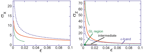
Figure 2: Temperature dependencies of the paraconductivity components (solid lines). Left panel shows the in-plane component in units of $e^{2}/(32\hbar\xi_{z,1})$ (function $\kappa(\epsilon)/\sqrt{\epsilon}$, see Eqs. (41) and (38)). This curve also gives the fluctuation specific heat in units $1/(8\pi\xi_{1,x}^{2}\xi_{1,z})$, see Eq. (37). Right panel shows the z-axis component in units of $e^{2}\xi_{z,1}/(32\hbar\xi_{x,1}^{2})$ calculated from Eq. (42). Both components were calculated using parameters $S_{12}=0.035$, $\widetilde{\theta}=0.377$ and $r=300$. For comparison we also show the Ginzburg-Landau asymptotics (dotted lines) and $\sigma$-band contribution to paraconductivity (dashed lines). One can see that in-plane component diverges slower and z-axis component diverges faster than the paraconductivity in a single-band anisotropic superconductor. In the $\sigma_{z}$-plot we indicate three characteristic regions with different functional dependencies of fluctuation parameters.

IV.2.2 z-component

The longitudinal component of paraconductivity $\sigma_{z}^{\prime}$ is given by the Eq. (40). Here the velocity renormalization turns out to be essential and it cannot be omitted. Performing integration with respect to $q_{\parallel}$ and using the introduced above reduced variable $u$, the result can be rewritten as

$$\sigma_{z}^{\prime}\approx\frac{e^{2}\xi_{1,z}}{32\hbar\xi_{1,x}^{2}\sqrt{\epsilon}}\int_{0}^{\infty}\frac{4du}{\pi}\frac{u^{2}\left[1+S_{12}r\tilde{\beta}^{\prime}_{2}(u)\right]^{2}}{\left[1+u^{2}+(S_{12}/\epsilon)\tilde{\beta}_{2}(u)\right]^{2}\,}.$$ (42)

In the Ginzburg-Landau regime, $\epsilon\ll 1/r+S_{12}$, we obtain

$$\sigma_{z}^{\prime}=\frac{e^{2}\xi_{1,z}\sqrt{1+S_{12}r}}{32\xi_{1,x}^{2}\sqrt{\epsilon}}.$$

In the regime of nonlocal fluctuations ($\epsilon\gg 1/r+S_{12}$), out of the GL region, the behavior $\sigma_{z}^{\prime}$ becomes quite peculiar. Essential contributions to the integral in Eq. (40) occur from two regions of $q_{z}$:  from $q_{z}\sim 1/\xi_{2,z}$ in arguments of functions $\tilde{\beta}_{2}$ and $\tilde{\beta}^{\prime}_{2}$ (mainly $\pi$-band contribution) and from $q_{z}\sim\sqrt{\epsilon}/\xi_{1,z}$ (mainly $\sigma$-band contribution). This corresponds to the ranges $u\sim 1/r\epsilon\ll 1$ and $u\sim 1$ in the reduced integral Eq. (42). We evaluate separately contributions from these ranges, or, what is the same, from $\pi$- and $\sigma$- bands in the most interesting case $rS_{12}\gg 1$ relevant for MgB₂.

In the range $u\sim 1/r\epsilon$ one can drop $\sigma$-band terms in Eq. (42). As we consider the regime $\epsilon\gg S_{12}$ we can neglect the term with $\tilde{\beta}$ in denominator. Dimensionalizing the integral, one can obtain the following result for this term

$$\sigma_{z,\pi}^{\prime} \approx\frac{e^{2}\xi_{1,z}S_{12}^{2}\sqrt{r}}{32\hbar\xi_{1,x}^{2}\epsilon^{2}}C_{2}(\tilde{\theta}),$$ (43)

$$C_{2}(\tilde{\theta}) =\int_{0}^{\infty}\frac{4dv}{\pi}v^{2}\left[\tilde{\beta}^{\prime}_{2}\left(v^{2}\right)\right]^{2}.$$

Numerical calculation gives $C_{2}(0)\approx 1.185$ and $C_{2}(0.377)\approx 0.235$.

In the range $u\sim 1$ the main contribution occurs from the $\sigma$-band and the terms proportional to $S_{12}$ ($\pi$-band terms) can be treated as small perturbations. Expansion with respect to these terms leads to the following result for the paraconductivity contribution

$$\sigma_{z,\sigma}^{\prime}\approx\frac{e^{2}\xi_{1,z}}{32\hbar\xi_{1,x}^{2}\sqrt{\epsilon}}\left(1+\frac{S_{12}}{2\epsilon}I_{z}\right)$$ (44)

with

$$I_{z}=\frac{16}{\pi}\int_{0}^{\infty}du\frac{u^{2}}{\left(1+u^{2}\right)^{2}}\left[\epsilon r\ \tilde{\beta}^{\prime}_{2}-\frac{\tilde{\beta}_{2}}{1+u^{2}}\right]$$

$$\approx-\frac{\ln\left(C_{3}r\epsilon\right)}{1+\tilde{\theta}\ln\left(C_{4}r\epsilon u^{2}\right)}.$$

with $C_{3}=16\pi^{-2}\gamma_{E}\exp(-4)\approx 0.053$ and $C_{4}\approx 2.9$. Let us note that in this range of temperatures the contribution from the $\pi$-band comes with the negative sign, as in the cases of the heat capacity and in-plane paraconductivity. This means that the $\pi$-band contribution changes sign with increasing temperature. Comparing contributions (43) and (44), we find that the $\pi$-band term dominates in the interval of temperatures $\epsilon<S_{12}\left(rS_{12}\right)^{1/3}$.

Therefore in the case $rS_{12}\gg 1\$ the $z$ axis paraconductivity $\sigma_{z}^{\prime}$ has three asymptotic regimes:

$$\sigma_{z}^{\prime}=\frac{e^{2}\xi_{1,z}}{32\hbar\xi_{1,x}^{2}\sqrt{\epsilon}}\left\{\begin{array}[c]{ll}\left(1+S_{12}r\right)^{1/2},&\text{for }\epsilon\ll 1/r+S_{12}\\ \sqrt{r}S_{12}^{2}C_{2}(\tilde{\theta})/\epsilon^{3/2},&\text{for }1/r+S_{12}\ll\epsilon\ll\frac{\left(rS_{12}\right)^{4/3}}{r}\\ 1-\frac{S_{12}}{2\epsilon}\frac{\ln\left(C_{1}r\epsilon\right)}{1+\tilde{\theta}\ln\left(C_{1}r\epsilon\right)},&\text{for }\max[1/r+S_{12},S_{12}\left(rS_{12}\right)^{1/3}]\ll\epsilon\ll 1\end{array}\right..$$ (45)

In the case $rS_{12}<1\$ the intermediate asymptotic disappears.

The right panel of Fig. 2 shows the numerically calculated dependence of $\sigma_{z}^{\prime}\left(\epsilon\right)$ with parameters specified in the captions. For comparison, we also show the GL asymptotics and the $\sigma$-band contribution.

V Final remarks

In this paper we have presented a microscopic derivation generalizing the conventional GL description onto two-band superconductors. We have further applied the developed approach to the investigation of the fluctuation phenomena in MgB₂. The important feature of our approach is that the derived nonlocal GL functional takes into account not only the long-wavelength fluctuations (as is the case of the conventional GL theory), but also the short-wavelength fluctuations, which enables to significantly extend the range of validity of the GL technique. This approach not only permits the study of the thermodynamic characteristics of the superconductors, but provides a convenient technique for calculation of transport coefficients.

It is necessary to underline that we succeeded to solve analytically the problem of accounting for short-wavelength fluctuations due to the specific for our model large difference in the intra-band diffusion coefficients $D_{\alpha}$. Fortunately, this assumption corresponds to the practically interesting case of magnesium diboride.

One can see that the main qualitative effect that determines the unusual behavior of fluctuations in the anisotropic two-band model consists in globalization of superconductivity in the immediate vicinity of transition temperature ($\epsilon\ll 1/r+S_{12}$). It occurs due to the possibility for electrons of both bands to participate in fluctuation pairing and to exchange of fluctuation pairs between them. Formally, this process manifests itself in the appearance of long range superconducting correlations on the scale $\widetilde{\xi}_{z}\gg\xi_{1,z}$.

Turning the role of fluctuations in MgB₂, we refer to the formulas for paraconductivity in a one-band 3D anisotropic superconductor LV02 :

$$\sigma_{x}^{\prime}=\frac{e^{2}}{32\hbar\sqrt{\epsilon}}\frac{\xi_{x}}{\xi_{y}\xi_{z}},\,\,\sigma_{z}^{\prime}=\frac{e^{2}}{32\hbar\sqrt{\epsilon}}\frac{\xi_{z}}{\xi_{x}\xi_{y}}.$$ (46)

We see that the growth of the effective $\widetilde{\xi}_{z}$ results in the noticeable increase of the $z$-axis paraconductivity in the immediate vicinity of critical temperature ($\epsilon\ll 1/r+S_{12}$) with respect to its high temperature ($\epsilon\geq S_{12}^{4/3}r^{1/3}$) extrapolation based only on the $\sigma$-band fluctuation pairing. The crossover between these two 3D regimes occurs in the narrow interval of temperatures $1/r+S_{12}\gg\epsilon\geq S_{12}^{4/3}r^{1/3}$ where the boson degrees of freedom corresponding to the pairings in $\pi$-band rapidly freeze out, leading to the fast decrease ($\sim\epsilon^{-2}$) of $z$-axis paraconductivity. We want to stress that this temperature dependence appears due to the noticeable contribution of short-wavelength fluctuations in this range of temperatures.

In the case of the in-plane component of paraconductivity and the fluctuation part of heat capacity, the situation is the opposite. The coherence length $\xi_{z}$ appears in the denominator of the corresponding expressions, so $\sigma_{x}^{\prime}$ and $C^{\prime}$ turn out to be suppressed in the vicinity of transition with respect to their extrapolation formulas from the high-temperature behavior. Similar situation occurs in the temperature dependencies of the in-plane upper critical field and of anisotropy of the upper critical field GK03a ; GK03b .

The obtained results coincide with that ones of the diagrammatic approach but the proposed GL description has an advantage of being more physically transparent, economic, and universal. The fact that the results derived via the GL equations coincide with those of our microscopic consideration is a convincing cross-check of the phenomenological description. The same approach can be used to derive other fluctuation properties such as the magnetic susceptibility and the field dependencies of conductivity and magnetization in the vicinity of transition.

VI Acknowledgements

This work was supported by the U.S. DOE, Office of Science, under contract # W-31-109-ENG-38. A.A.V. acknowledges the support of the FIRB project of the Italian Ministry of Science and Education.

References

- (1) V. L. Ginzburg and L. D. Landau, Zh. Eksp. Teor. Fiz. , 20, 1064(1950).
- (2) A. A. Abrikosov, Zh. Eksper. i Teor. Fiz. 32, 1442(1957) (Sov. Phys. JETP 5, 1174(1957)).
- (3) G. Blatter, M. V. Feigel’man, V. B. Geshkenbein, A. I. Larkin, and V.M.Vinokur, Rev. of Mod. Phys., 66, 1180(1994).
- (4) L.Viverit, G.M.Brun, A.Minguzzi, and R. Fazio, Pairing fluctuations in trapped Fermi gases, cond-mat/0402620 v1 (2004).
- (5) L. P. Gor’kov, Zh. Eksp. Teor. Fiz. 36, 1918, (1959) [Sov. Phys. JETP, 9, 1364 (1959)]; L. P. Gor’kov and T. K. Melik-Barkhudarov, Zh. Eksp. Teor. Fiz. 45, 1493, (1963) [Sov. Phys. JETP, 18, 1031 (1964)].
- (6) A. A. Golubov and A. E. Koshelev, Phys. Rev. B 68, 104503 (2003).
- (7) A. E. Koshelev and A. A. Golubov, Phys. Rev. Lett. 92, 107008 (2004).
- (8) Yu. Eltsev, S. Lee, K. Nakao, N. Chikumoto, S. Tajima, N. Koshizuka, and M. Murakami, Phys. Rev. B 65, 140501(R) (2002); Physica C 378-381, 61 (2002). L. Lyard, P. Samuely, P. Szabo, T. Klein, C. Marcenat, L.Paulius, K.H.P. Kim, C.U. Jung, H.-S. Lee, B. Kang, S. Choi, S.-I. Lee, J. Marcus, S. Blanchard, A.G.M. Jansen, U. Welp, G. Karapetrov, W.K. Kwok., Phys. Rev. B 66, 180502(R) (2002); M. Angst, R. Puzniak, A. Wisniewski, J. Jun, S. M. Kazakov, J. Karpinski, J. Roos, and H. Keller, Phys. Rev. Lett. 88, 167004 (2002).
- (9) A. A. Abrikosov, L. P. Gorkov, and I. E. Dzyaloshinski, Methods of quantum field theory in statistical physics, Prentice-Hall, Inc., Englewood Cliffs, NJ, 1963.
- (10) Strictly speaking, the band structure of MgB2 is composed of four bands: two bands and two -bands (see, e.g., Ref. LiuPRL01, ). However, in real samples the scattering rate between the bands of the same family is usually high while the scattering of electrons between the different families is rather weak.M03 In this situation scattering homogenizes superconductivity inside both band families and superconductivity in magnesium diboride is effectively described by the two-band model. To simplify terminology, in the rest of the paper we use term “-band” (“-band”) for the family of -bands (-bands).
- (11) A. Larkin and A. Varlamov, Theory of fluctuations in superconductors, Oxford University press (2004).
- (12) G. M. Eliashberg, Zh. Eksp. i Teor. Fis. 41, 1241 (1961) [ Sov. Phys. - JETP , 14, 856 (1961)].
- (13) R. H. T. Wilke, S. L. Bud’ko, P. C. Canfield, D. K. Finnemore, R. J. Suplinskas, and S. T. Hannahs,Phys. Rev. Lett. 92, 217003 (2004); V. Braccini, et al. cond-mat/0402001; M. Angst, S. L. Bud’ko, R. H. T. Wilke, P. C. Canfield cond-mat/0410722
- (14) I. I. Mazin, O. K. Andersen, O. Jepsen, O. V. Dolgov, J. Kortus, A. A. Golubov, A. B. Kuz’menko, and D. van der Marel, Phys. Rev. Lett. 89 107002 (2002).
- (15) H. Suhl, B. T. Matthias, and L. R. Walker, Phys. Rev. Lett. 3, 552 (1959).
- (16) V. A. Moskalenko, Fiz. Met. Met. 4, 503 (1959).
- (17) J. Kortus, I. I. Mazin, K. D. Belashchenko, V. P. Antropov, L. L. Boyer, Phys. Rev. Lett. 86, 4656 (2001).
- (18) J. N. An and W. E. Pickett, Phys. Rev. Lett. 86, 4366 (2001).
- (19) A. Y. Liu, I. I. Mazin, and J. Kortus, Phys. Rev. Lett. 87, 087005 (2001).
- (20) Y. Kong, O. V. Dolgov, O. Jepsen, and O. K. Andersen , Phys. Rev. B 64, 020501(R) (2001).
- (21) T. Yildirim, O. Gülseren, J. W. Lynn, C. M. Brown, T. J. Udovic, Q. Huang, N. Rogado, K. A. Regan, M. A. Hayward, J. S. Slusky, T. He, M. K. Haas, P. Khalifah, K. Inumaru, and R. J. Cava , Phys. Rev. Lett. 87, 037001 (2001).
- (22) H. J. Choi, D. Roundy, H. Sun, M. L. Cohen, and G. Louie, Phys. Rev. B, 66, 020513 (2002); Nature 418, 758 (2002).
- (23) A. A. Golubov, J. Kortus, O. V. Dolgov, O. Jepsen, Y. Kong, O. K. Andersen, B. J. Gibson, K. Ahn, and R. K. Kremer, J.Phys.: Condens. Matter, 14, 1353 (2002).
- (24) K. Maki, Physics, 1, 21 (1964).
- (25) A. Carrington and F. Manzano, Physica C, 385, 205 (2003).
- (26) J. Kortus, O. V. Dolgov, R. K. Kremer, and A. A. Golubov, cond-mat/0411667
- (27) A. S. Sidorenko, L. R. Tagirov, A. N. Rossolenko, N. S. Sidorov, V. I. Zdravkov, V. V. Ryazanov, M. Klemm, S. Horn, and R. Tidecks, JETP Letters 76, 17 (2002).