Spatial patterns and scale freedom in a Prisoner’s Dilemma cellular automata with Pavlovian strategies

A cellular automaton in which cells represent agents playing the Prisoner’s Dilemma (PD) game following the simple ”win-stay, loose-shift” strategy is studied. Individuals with binary behavior, such as they can either cooperate (C) or defect (D), play repeatedly with their neighbors (Von Neumann’s and Moore’s neighborhoods). Their utilities in each round of the game are given by a rescaled payoff matrix described by a single parameter $\tau$, which measures the ratio of temptation to defect to reward for cooperation. Depending on the region of the parameter space $\tau$, the system self-organizes - after a transient - into dynamical equilibrium states characterized by different definite fractions of C agents $\bar{c}_{\infty}$ (2 states for the Von Neumann neighborhood and 4 for Moore neighborhood). For some ranges of $\tau$ the cluster size distributions, the power spectrums $P(f)$ and the perimeter-area curves follow power-law scalings. Percolation below threshold is also found for D agent clusters. We also analyze the asynchronous dynamics version of this model and compare results.

keybords: Complex adaptive systems, Sociophysics, Econophysics, Agent-based models, Self-organized criticality.

PACS numbers: 89.75.-k, 89.20.-a, 89.65.Gh, 02.50.Le, 87.23.Ge

1 Introduction

The Prisoner’s Dilemma (PD) game plays in Game Theory a role similar to the harmonic oscillator in Physics. Indeed, this game, developed in the early fifties, offers a very simple and intuitive approach to the problem of how cooperation emerges in societies of ”selfish” individuals i.e. individuals which pursue exclusively their own self-benefit. It was used in a series of works by Robert Axelrod and co-workers [1] to examine the basis of cooperation in a wide variety of contexts. Furthermore, approaches to cooperation based on the PD have shown their usefulness in Political Science [2]-[4], Economics [5]-[11], International Affairs [12]-[15], Theoretical Biology [16]-[18] and Ecology [19]-[20].

The PD game consists in two players each confronting two choices: cooperate (C) or defect (D) and each makes his choice without knowing what the other will do. The four possible outcomes for the interaction of both agents are: 1) they can both cooperate: (C,C), 2) both defect: (D,D), 3) one of them cooperate and the other defect: (C,D) or (D,C). Depending on the case 1)-3), the agents get respectively : the ”reward” $R$, the ”punishment” $P$ or the ”sucker’s payoff” $S$ the agent who plays C and the ”temptation to defect” $T$ the agent who plays D. These four payoffs obey the relations:

$$T>R>P>S$$

and

$$2R>S+T.$$ (1)

The last condition is required in order that the average utilities for each agent of a cooperative pair ($R$) are greater than the average utilities for a pair exploitative- exploiter (($R+S$)/2). One can assign a payoff matrix M to the PD game given by

$${\mbox{M}}=\left(\matrix{(R,R)&(S,T)\cr(T,S)&(P,P)\cr}\right),$$

which summarizes the payoffs for row actions when confronting with column actions. Clearly it pays more to defect: if one of the two players defects -say $i$- , the other who cooperates will end up with nothing. In fact, even if agent $i$ cooperates, agent $j$ should defect, because in that case he will get $T$ which is larger than $R$. That is, independently of what the other player does, defection D yields a higher payoff than cooperation and is the dominant strategy for rational agents. Furthermore, is the Nash equilibrium [21] - i.e. a best reply to itself - of the PD game. The dilemma is that if both defect, both do worse than if both had cooperated: both players get $P$ which is smaller than $R$. A possible way out for this dilemma is to play the game repeatedly. In this iterated Prisoner’s Dilemma (IPD), there are several strategies that outperform the dominant [D,D] one-shot strategy and lead to some non-null degree of cooperation.

The attainment of cooperation in PD simulations relies on different mechanisms and factors. A popular point of view regards direct reciprocity as the crucial ingredient. A typical exponent of this viewpoint is the strategy known as Tit for Tat (TFT): cooperate on the first move, and then cooperate or defect exactly as your opponent did on the preceding encounter. This requires either memory of previous interactions or features (”tags”) permitting cooperators and defectors to distinguish one another [22].

Spatial structure has also been identified as an influential factor in building cooperation. For instance, in ref. [23] the authors neglected all strategical complexities or memories of past encounters. Instead, they show that spatial effects by themselves in a classic Darwinian setting are sufficient for the evolution of cooperation .

The problem of cooperation is approached mainly from an Darwinian evolutionary perspective: strategies that incorporate some dose of cooperative behavior are the most successful and propagate displacing competing strategies that do not. In that sense, a central concept is that of evolutionary stable strategy (ESS) [24], [25]: a strategy which if adopted by all members of a population cannot be invaded by a mutant strategy through the operation of natural selection. The evolutionary game theory, originated as an application of the mathematical theory of games to biological issues, later spread to economics and social sciences.

In this work, we follow a different approach: there is no competition of different strategies, all the agents follow a natural strategy of ”win-stay, loose-shift” known as Pavlov [26]. We do not worry about the resistance of the strategy against invasion by other strategies (like unconditional defectors or ALL D that play D independently of what the opponent does), rather we take Pavlov for granted. The rationale for this relies on several facts. First, Pavlov seems to be a widespread strategy in nature [27]. Second, Pavlov does pretty well when competing with several other strategies including generous tit-for-tat GTFT as it was shown by Nowak and Sigmund [28]. Moreover, they found that in a non-spatial setting while Pavlov can be invaded by ALL D a slightly stochastic variant cannot. Third, experiments with humans have shown that a great fraction of individuals indeed use Pavlovian strategies [29].

Therefore, we address the analysis of the self-organized states that emerge when simple agents, possessing neither long term memory nor tags, play the PD game in a spatial setting using Pavlov strategy. We this aim we resort to a cellular automaton in which each cell is either black or white representing, respectively, a D or a C agent. Each agent plays with those belonging to his neighborhood, and the total utilities he gets determine the update of his individual state.

We consider payoff matrices implying strict dilemmas defined by equations (1) rather than weak ones in which the inequalities are relaxed (for instance $P=S$). To simplify things we parameterize the payoff matrix in terms of a single parameter $\tau$, which measures the ratio of temptation to defect to reward for cooperation.

Different self-organizations occur depending on the value of $\tau$, the type of dynamics and the considered neighborhood. In particular, for a range of values of $\tau$ (that depends on the neighborhood) we found power law behavior that might be a signature of self-organized criticality [30].

Previously, a non spatial similar model, in which pairs of agents were chosen at random, was analyzed in ref. [31]. Also, a Mean Field stochastic version was considered in [32].

This work is organized as follows. In section 2 we describe the model. In section 3 we present the results of simulations as well as analytical results obtained by using a Mean Field approximation that neglects all spatial correlations (details in the appendix at the end). Section 4 is devoted to conclusions and final remarks.

2 The Model

The model is vey simple: we assign to each agent, located at the cell with center at $(x,y)$, a binary behavioral variable $c(x,y)$ which takes the value ”1” for C agents and ”0” for D agents. This agent plays with the $z$ agents belonging to his neighborhood $N(x,y)$ getting a payoff $U_{1}(x,y)$ with the first neighbor he plays, $U_{2}(x,y)$ with the second one and so on . The total utilities $U(x,y)=U_{1}(x,y)+U_{2}(x,y)+...+U_{z}(x,y)$ he gets playing with his neighborhood determine the update of his individual state. More technically, we have an outer totalistic cellular automaton i.e. the state of a cell at the next time-step depends only on its own state, and the sum of the states of its neighbors. The dynamic is synchronous: all the agents update their states simultaneously at the end of each lattice sweep. In addition to this synchronous dynamics or ”parallel updating” we also explored, with less detail, the asynchronous dynamics or ”sequential updating”, in which the state of an agent is updated after he played.

We considered two different neighborhoods: a) the von Neumann neighborhood ($z=4$ neighbor cells: the cell above and below, right and left from a given cell) and b) the Moore neighborhood ($z=8$ neighbor cells: von Neumann neighborhood + diagonals).

The payoff matrix is parameterized in terms of a single parameter $\tau\equiv T/R$:

$${\mbox{M}}=\left(\matrix{(1,1)&(-\tau,\tau)\cr(\tau,-\tau)&(-1,-1)\cr}\right),$$ (2)

with $\tau>1$. The total utilities of the agent at $(x,y)$ at time $t$, $U(x,y,t)$, are the sum of the utilities collected by playing with each of his neighbors, as prescribed by the payoff matrix.

A typical value for the population of agents is $N_{ag}=10,000$ (100 $\times$ 100 lattice).

The initial state at $t=0$ is taken as $c(x,y;0)=0$ or $1$ (D or C respectively), chosen at random for each cell $(x,y)$. Then the system evolves by iteration during $t_{f}$ time steps till it reaches a stationary or dynamical equilibrium state.

Pavlov’s strategy works as follows. The agent at $(x,y)$ will change his state for the next time step $t+1$: $c(x,y,t+1)=1-c(x,y,t)$ (from C to D or viceversa) if $U(x,y,t)<0$, and will remain the same: $c(x,y,t+1)=c(x,y,t)$, if $U(x,y,t)>0$ (when $U(x,y,t)=0$ the agent changes with probability 0.5). Once all the agents have played, their state is updated for the next time iteration.

For the von Neumann neighborhood then, each agent plays with his four nearest neighbors. Let’s analyze what is expected to happen for different values of the parameter $\tau$. Let’s focus on the agent at $(x,y)$ and his possible configurations (C or D) and the ones of his neighborhood (number of C and D neighbors) and in each case his corresponding utilities. These results are shown in Table 1:

	4C, 0D	3C, 1D	2C, 2D	1C, 3D	0C, 4D
C	4	3-$\tau$	2-2$\tau$	1-3$\tau$	-4$\tau$
D	4$\tau$	3$\tau$ -1	2$\tau$-2	$\tau$-3	-4

Table 1. Utilities of a given agent depending if his state is C (row 1) or D (row 2) and the states of his neighborhood (columns 2 to 6) for von Neumann neighborhood.

From Table 1, since $\tau>1$, we observe that the sign of the utilities $U(x,y)$ of the agent located at site $(x,y)$ -which determines the update of his $c(x,y)$- depends on the value of $\tau$ only for two cases: a) if the agent plays C and his neighborhood consists in 3C agents and 1D or b) if the agent plays D and his neighborhood consists in 1C agent and 3D agents. In both cases the update rule depends thus whether $\tau>3$ or $\tau<3$. So, a priori, one would expect the existence of a ”critical” value of the parameter $\tau^{*}=3$ such that the results depend on whether $\tau$ is greater or smaller than this critical value. Intuitively one can argue that since for $\tau>3$ there are more favorable situations for D agents and disfavorable for C agents, the mean cooperation of the system when the dynamical equilibrium is reached, $c_{\infty}=\frac{1}{N_{ag}}\sum_{{N_{ag}}}\,c(x,y,t)$ -after the transient-, will be smaller than when $\tau<3$.

Table 2 summarizes the utilities of a player for each possible configuraqtion of his neighbors for the case of Moore neighborhood.

	8C, 0D	7C, 1D	6C, 2D	5C, 3D	4C, 4D	3C, 5D	2C, 6D	1C, 7D	0C,8D
C	8	7-$\tau$	6-2$\tau$	5-3$\tau$	4-4$\tau$	3-5$\tau$	2-6$\tau$	1-7$\tau$	-8$\tau$
D	8$\tau$	7$\tau$ -1	6$\tau$-2	5$\tau$-3	4$\tau$-4	3$\tau$ -5	2$\tau$-6	$\tau$-7	-8

Table 2. The same as Table 1 but for Moore neighborhood.

A completely analogous reasoning for the Moore neighborhood leads to three ”critical” values: $\tau^{*}_{1}=5/3$, $\tau^{*}_{2}=3$ and $\tau^{*}_{3}=7$. Here we would expect also that $c_{\infty}$ will diminish as $\tau$ crosses each frontier value $\tau^{*}_{i}$ from left to right.

3 RESULTS

To avoid dependence on the initial conditions the measures correspond to averages taken over an ensemble of 100 systems with arbitrary initial conditions. In general, the results for the asymptotic regime, after a transient, become almost independent of the lattice size $L$ for $L~{}\raise 1.72218pt\hbox{$>$}\hbox to0.0pt{\hss\lower 2.58334pt\hbox{$\sim$}}~{}100$. Therefore in what follows, unless it is stated otherwise, the results correspond to simulations performed in $100\times 100$ lattices.

As we have anticipated, we observe that the stationary state of the system changes as the parameter $\tau$ moves from one region to another (two regions in the case of $z=4$ von Neumann neighborhood and four regions for $z=8$ Moore neighborhood).

3.1 Asymptotic average fraction of cooperators $\bar{c}_{\infty}$

The asymptotic or equilibrium mean fraction of C-agents $\bar{c}_{\infty}$, takes constant values in each of the regions delimited by the ”critical” $\tau^{*}$. Hence we have one sharp step at $c_{\infty}=3$ for $z=4$ and three sharp steps at $c_{\infty}=\frac{5}{3}$, 3 $\&$ 7 for $z=8$.

It is interesting to compare the $\bar{c}_{\infty}$, produced by simulations, with the $c^{MF}_{\infty}$ obtained by elementary calculus using a Mean Field (MF) approximation that neglects all spatial correlations (see APPENDIX I).

In Tables 3 and 4 we present the $\bar{c}_{\infty}$ and $c^{MF}_{\infty}$ for $z=4$ and $z=8$ respectively. Clearly, as expected, the MF approximation improves increasing $z$. In addition, divergences between spatial games and the MF approximation become maximum in the ”cooperative” sector of the parameter $\tau$ (leftist region, producing $c_{\infty}~{}\raise 1.72218pt\hbox{$>$}\hbox to0.0pt{\hss\lower 2.58334pt\hbox{$\sim$}}~{}0.5$ ). This can be explained in terms of the particular cluster structure of that region exhibiting power law scalings (see next subsection).

z=4	Simulations	MF
$\tau<3$	$0.485\pm 0.002$	0.430
$\tau\geq 3$	$0.280\pm 0.002$	0.342

Table 3. The asymptotic fraction of cooperators $c_{\infty}$ for $z=4$ von Neumann neighborhood. Column 2: simulations. Column 3: MF approximation (see APPENDIX I).

z=8	Simulations	MF
$1<\tau<5/3$	$0.563\pm 0.002$	0.461
$5/3\leq\tau<3$	$0.436\pm 0.002$	0.420
$3\leq\tau<7$	$0.366\pm 0.003$	0.386
$8\leq\tau$	$0.320\pm 0.003$	0.334

Table 4. The asymptotic fraction of cooperators $c_{\infty}$ for $z=8$ More neighborhood. Column 2: simulations. Column 3: MF approximation (see APPENDIX I).

3.2 Spatial Patterns: The Cluster Structure

Von Neumann neighborhood

In Fig. 1 we present snapshots -after the transient- of the cellular automaton for $\tau<3$ and $\tau>3$. These ”cooperation maps” illustrate the differences between the typical spatial patterns that arise in the two parameter regions divided by $\tau*=3$.

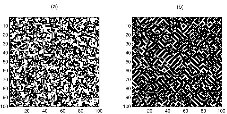
Figure 1: Asymptotic ”cooperation maps” for: (a) $\tau<3$, (b) $\tau>3$. Black=D, white=C.

For $\tau<3$ we found that:

I) Although the asymptotic probability for D agents is $\bar{d}_{\infty}=1-\bar{c}_{\infty}\simeq 0.5$, which is below the percolation threshold $p_{c}\approx 0.59275$, giant spanning D clusters often occur. Percolation below threshold is a known fact in other models. In general, when there are correlations between the sites, the threshold is shifted. As it happens, for instance, in the square Ising model percolation occurs, at the critical temperature, when the concentration is also 0.5.

II) Different quantities behave as power laws implying thus the emergence of scale free phenomena. For instance, the size distribution of clusters of D agents exhibits power law scaling.

For $\tau>3$ the distribution of D clusters is bimodal with a peak for very small clusters (size=1) and a secondary peak for very large clusters. The main peak for very small clusters can be explained by the small correlation length. On the other hand, the secondary peak for very large sizes arises because the probability of a given site to be in the D state $\bar{d}_{\infty}\equiv 1-\bar{c}_{\infty}$ is over the site percolation threshold and thus spanning clusters are much more abundant than when $\tau<3$ in which case $\bar{d}_{\infty}<p_{c}$.

Fig. 2 is a plot of the log of the number of clusters of C and D agents vs. the log of their size for $\tau<3$ and $\tau>3$ using $400\times 400$ lattices. In both cases giant spanning clusters of D agents were excluded. This, in particular for $\tau>3$, eliminates a large number of clusters belonging to the secondary peak of its bimodal distribution and explains why there are less ”+” points in Fig.2- (b) than in 2-(a) (the shortage of ”*” points, representing C clusters, obviously is related to the fact that $c_{\infty}$ is smaller on the $\tau>3$ side).

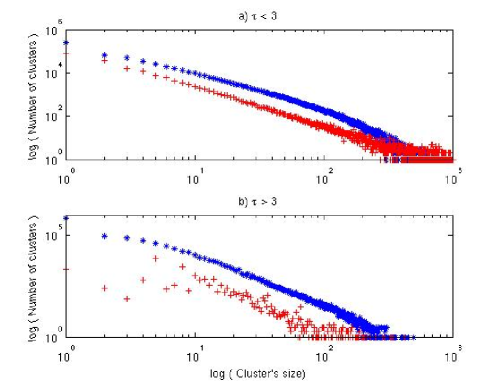
Figure 2: Number of clusters of C (*) and D (+) agents vs. size of the clusters for the von Neumann neighborhood in a 400$\times$400 lattice. The clusters are summed over the last 150 lattice sweeps after the transient for: (a) $\tau<3$, (b) $\tau>3$. In both cases giant spanning D clusters were not included

The data points for D clusters seem consistent with a power law scaling over a couple of decades, with a critical exponent of approximately $-1.79\pm 0.02$. The graphic also shows a difference between C and D clusters: the first ones exhibit much greater deviations from an exact power law although they also occur over a wide range of scales. This asymmetry can be traced to the difference that exists for the possible stable configurations of clusters of C’s or D’s; while the first ones need at least three C neighbors to remain C, the second ones can do well with only two C neighbors. Then the D agents can form thinner clusters than the C agents. This fact increases the probability of agents D to yield larger clusters. This also can explain why although the equilibrium probability for D agents is below the percolation threshold, giant spanning D clusters are observed.

For $\tau>3$ the situation changes drastically as Fig. 2.(b) reflects, here it can be seen that the data don’t fit well with a power law neither for D nor for C clusters.

Remark - To check that the power law scaling is not dependent on the particular parameterization of the payoff matrix we are using, we measured the cluster distribution for many other payoff matrices not described by (2). For instance, we considered this alternative parameterization of the payoff matrix

$${\mbox{M}^{\prime}}=\left(\matrix{(1,1)&(\tau/2-3,\tau)\cr(\tau,\tau/2-3)&(-1,-1)\cr}\right),$$

with $3-\tau/2<-1<1<\tau$ Again, we found power law behaviour for the leftist region in $\tau$. Thus, it seems that this power law scaling for an entire collection of PD payoff matrices is a robust property of the model.

Another clue about the dynamics of the clusters can be obtained by examining the relation of the perimeter to the area of the clusters. We define the perimeter of a cluster C (D) as the set of sites $(x,y)$ with behavioral variable $c(x,y)=1$ ($c(x,y)=0$) belonging to the cluster with at least one neighbor with the opposite behavioral variable i.e. $c(x,y)=0$ ($c(x,y)=1$). The mean perimeter $P(A)$, for a given area $A$, is then given by averaging over all the perimeters of clusters with area $A$. Fig.3 shows that for $\tau<3$ the perimeter scales linearly with the area, that is, at the fastest rate possible, implying that the clusters are highly ramified. The fraction of the area that is interior to the clusters can be easily calculated.

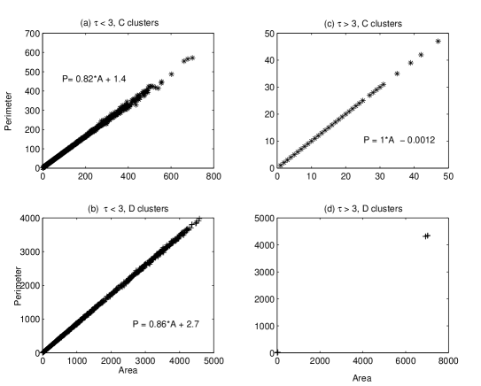
Figure 3: Perimeter vs. area of the clusters of C and D agents for z=4. The perimeter’s values plotted are averages of perimeters of clusters of the same size, taken over the last 500 lattice sweeps after the transient.

By fitting the point of Figs.3.(a) and (b) we get the following expressions for the perimeter as a function of the area, for $\tau<3$:

$$\begin{array}[]{ll}P_{C}\approx 0.82A_{C}&\quad\mbox{for clusters of C agents}\\ P_{D}\approx 0.86A_{D}&\quad\mbox{for clusters of D agents}.\par\end{array}$$ (3)

Then the cluster interior fraction is $F=\frac{A-P}{A}$. Thus we get that approximately:

$$\begin{array}[]{ll}F_{C}\simeq 0.18&\quad\mbox{for clusters of C agents}\\ F_{D}\simeq 0.16&\quad\mbox{for clusters of D agents}\par\end{array}$$ (4)

This shows that the clusters have almost no interior, and confirms our previous observation concerning that the clusters of D agents are thinner than those of C agents. This supports quantitatively the explanation of why percolation of D agents is observed but no of C agents. The linear behavior shown in Fig.3.(c), which slope approximatelly equal to 1, can be understood by inspection of Fig.1.(b) where is clearly seen that the C agents form small ”laddered” clusters in which the perimeter is equal to the area.

Moore neighborhood

For arbitrary random initial conditions, the equilibrium cooperation maps are shown in Fig.4 for $\tau$ in the different regions of interest.

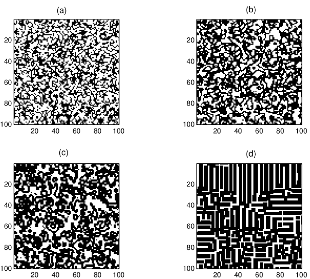
Figure 4: Cooperation maps for Moore neighborhood at equilibrium (after $10^{5}$ iterations) for: (a) $\tau\in(1,\frac{5}{3})$, (b) $\tau\in(\frac{5}{3},3)$, (c) $\tau\in(3,7)$ and (d) $\tau>7$. Black=D, white=C.

As it can be seen from Table 4, when $\tau$ is within the interval $(1,\frac{5}{3})$, $\bar{c}_{\infty}\simeq 0.6$ which is higher than the values obtained for the von Neumann neighborhood for any $\tau$. This implies that increasing the number of neighbors in general produces a higher fraction of cooperators, although this higher value of $\bar{c}_{\infty}$ is stable for narrower domain values of $\tau$. We checked this for the case in which 12 neighbors are taken into account, achieving a value of $\bar{c}_{\infty}\simeq 0.8$ for $\tau\in(1,\frac{7}{5})$.

Let us analyze what happens to the clusters of C’s and D’s for the different values of $\tau$, this time for the Moore neighborhood. The results are shown in Fig. 5.

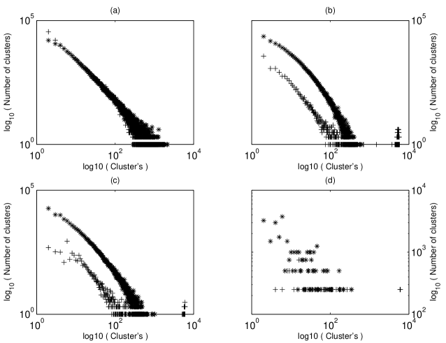
Figure 5: Number of clusters of C(*) and D(+) agents vs. size of the clusters, summed over the last 500 times after $10^{4}$ iterations for $z=8$, in logarithmic scale. The plots correspond to: (a) $\tau\in(1,\frac{5}{3})$, (b) $\tau\in(\frac{5}{3},3)$, (c) $\tau\in(3,7)$, (d) $\tau>7$. There is a percolation peak for clusters of D agents in (b), (c) and (d) since they are above the percolation threshold ($d>p_{c}$).

In Fig.5.(a), corresponding to $\tau\in(1,\frac{5}{3})$ and $c_{\infty}\simeq 0.57$, we can observe power law behavior for both clusters of C and D agents, with the same critical exponent of approximately $-1.62\pm 0.02$. This symmetry between C’s and D’s is broken when we take $\tau\in(\frac{5}{3},3)$ (Fig.5.(b), $c_{\infty}\simeq 0.44$): here we recover the kind of behavior we found for $\tau<3$ in the case of the von Neumann neighborhood (see Fig. 2.(a)), for which the power law scaling for D agents is much more claear than for C agents. In this case we find an exponent of approximately $-1.98\pm 0.04$. Remarkably, criticality seems to persist, although not so clearly as in the previous cases, even for values of $\tau$ in the interval $(3,7)$ (Fig.5.(c)). For $\tau>7$, power law behavior is completely lost, as Fig.5.(d) shows.

3.3 Power Spectrums

The power laws we found for spatial observables might be interpreted as signatures of self-organized criticality (SOC). In order to elucidate the criticality or not of the dynamics we analyzed temporal correlations. Specifically, we calculated the power spectrum $P(f)$ (i.e. the absolute value of the Fourier transform) of the time autocorrelation function $G(t)$ of the cooperative fraction $c(t)$. $G(t)$ is defined as:

$$G(t)\equiv<c(t_{0})c(t_{0}+t)>-<c(t_{0})>^{2},$$ (5)

where the average is taken over all possible temporal origins $t_{0}$.

It turns out that although the transients are not very long, $P(f)$ exhibits power law behavior, for the same range of values of $\tau$ we found this type of behavior for the cluster size distributions, for almost two decades. For instance, in the case of the von Neumann neighborhood, we have a power law power spectrum for $\tau<3$ which is lost for $\tau>3$ (which is consistent with the fact that the simulations have shown that for this region the system behaves periodically, with a very short period). This is shown in Fig.6.

The correlation function $G(t)$ is calculated for the transient. In order to maximize this transient an initial $c(t=0)=0.1$ very different from the known equilibrium value of $c_{\infty}\simeq 0.5$ was taken together with a large lattice of $1000\times 1000$.

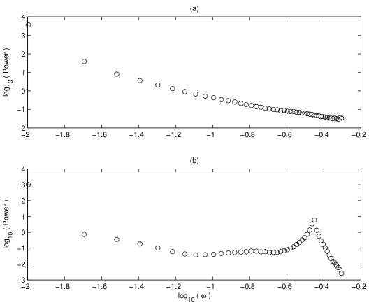
[h]

Figure 6: Power spectrum for $z=4$ Von Neumann neighborhood : (a) $\tau<3$, (b) $\tau>3$.

This power law scaling of $P(f)$, for the same region we found this type of behavior for the cluster sizes, can be interpreted as another signature for the possible existence of critical dynamics.

3.4 Asynchronous dynamics

As we mentioned in the previous section, besides exploring the synchronous dynamics, we also performed some runs using the asynchronous dynamics, in which the state of each agent is updated after he played with his neighborhood.

The asynchronous update produce a much less interesting situation. The power laws are lost, both for the von Neumann and Moore neighborhoods: we find no power laws for the cluster sizes nor for the power spectrum and the cooperation values decrease significantly. Still, there is a change in the mean value of the cooperation as the parameter $\tau$ goes through the critical values calculated earlier. For the von Neumann neighborhood, for $\tau<3$, $\bar{c}_{\infty}\simeq 0.34$. For $\tau>3$ cooperation decreases to $\bar{c}_{\infty}\simeq 0.23$ and there is no clear pattern of behavior. For the Moore neighborhood results are similar, with $\bar{c}_{\infty}\simeq 0.34$, $0.30$, $0.21$ and $0.13$ for $\tau\in(1,\frac{5}{3})$, $(\frac{5}{3},3)$, $(3,7)$ and $\tau>7$ respectively.

4 CONCLUSIONS

For a cellular automata, representing a system of agents playing the IPD governed by Pavlovian strategies in a simple territorial setting, we explored its steady states for different values of the parameter $\tau$ , which measures the ratio of temptation to defect to reward. Both for the Von Neumann and Moore neighborhoods we found sharp steps for $\bar{c}_{\infty}$ vs. $\tau$ (one step in the first case and three steps in the second case).

We found power-law scaling for different quantities, measuring either spatial (cluster size distributions) or temporal correlation ($P(f)$), for entire regions in parameter $\tau$ space. All this may be interpreted as consistent evidences of self-organized criticality in a spatial game which is not evolutionary (at least in the ordinary Darwinian sense). This result, which is qualitatively robust against changes of the payoff matrix and the neighborhood, is novel (as far as we know). [It is worth to mention that the parameterization (3.2) allows to study two other games besides the PD: If $-1<\tau<1$ ($R>T>P>S$) the game is known as ”Stag Hunt” (SH) while when $4<\tau<8$ ($T>R>S>P$) the game is called the ”Hawk-Dove” (H-D). We simulated these two games, which are popular in Social Sciences and Biology respectively, and, in contrast to what happen with the PD, we found no power law behavior [35].] On the other hand, the occurrence of critical dynamics in certain spatial evolutionary games has been observed. For instance, in ref. [33] it was shown that for certain range of a parameter, which determines the punishment, the spatial HD game exhibits large temporal and spatial correlations and various processes governed by power-laws. This is in contrast with the simplified version of the PD considered in ref. [23], which does not exhibit complex critical dynamics of this type, rather it has periodic or chaotic dynamics. Nevertheless, for a stochastic version of this evolutionary weak dilemma, power law behavior consistent with directed percolation has been measured [34].

We also have shown that percolation below the threshold value occurs for D-agents for the case of the von Neumann neighborhood. The asymmetry between C and D clusters, even in cases in which both types of agents appear with equal probability, can be explained in terms of the Pavlovian strategy and the asymmetry of the payoffs (see Table 1).

A result worth remarking is that the degree of cooperation can be increased by enlarging the neighborhood but, simultaneously, the temptation parameter $\tau$ must be restricted to smaller values.

Another interesting general result is the effect of changing the dynamics from synchronous to asynchronous. The scale invariance we found for the synchronous update disappear when we turn to the asynchronous update. The fact that the general qualitative behavior of asynchronous models may differ greatly from that of the synchronous version was noticed in [36].

Let us mention some interesting future extensions of the work presented here. For instance, we observed that for small lattices this simple deterministic system often reaches true equilibrium configurations, in which all the agents are happy (all get utilities above 0) and do not change their respective states. In other words, Pareto Optimal states ($POS$) i.e. states in which none of the players can increase their payoff without decreasing the payoff of at least one of the other players. In Fig.7 an example of such equilibrium states is presented for a small ($6\times 6$) lattice, $z=4$ and $\tau=2$.

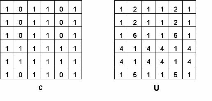
Figure 7: Pareto Optimal states configuration for a small $6\times 6$ lattice, $z=4$ and $\tau=3$. Left: the $c(i,j)$ matrix. Right: the corresponding utilities $U(i,j)$: the utilities for all the agents are positive and thus they don’t change their behavioral variables.

When the lattice size grows the system becomes unable to reach these $POS$. The explanation we found for this is , as the size grows, the fraction of $POS$ with respect to the possible configurations decreases. Additionally, it is plausible that the entirely deterministic update does not provide a path in configuration space connecting the initial state with an $POS$. The introduction of noise in the update rule, in some particular cases, might help promoting ergodicity. The effect of the introduction of noise in spatial evolutionary games was analyzed for example in [38] and [39]. An interesting goal is how to use noise to avoid entrainment in non efficient states i.e. to implement a sort of simulated annealing approach [37] allowing to reach these optimal equilibriums.

Another issue that seems worth exploring is the extension of the present approach, beyond the PD game, to games that are useful to model other different everyday situations, like the ”Stag Hunt”, ”Chicken”, etc [35].

Finally, after we concluded this manuscript, one of the referees pointed out the study of the PD game of Posch et al [40] using ”win-stay, lose-shift” strategies in a non spatial setup. This work offers an stimulating discussion of when can satisficing become optimizing.

Acknowledgments.

We are grateful to Professor Dietrich Stauffer for useful comments on percolation. S.V. wish to thank D.Guerra for sharing his programming skills.

APPENDIX I: MEAN FIELD COMPUTATIONS

Estimate of $c_{\infty}$ can be obtained by elementary calculus using a Mean Field approximation that neglects all spatial correlations.

Once the stationary state was reached, the transitions from D to C, on average, must equal those from C to D. Thus, the average probability of cooperation $c_{\infty}$ is obtained by equalizing the flux from C to D, $J_{CD}$, to the flux from D to C, $J_{DC}$. The possible utilities for a C player range from $R=z\times 1=z$ to $S=-z\tau$ (see Table 1 and Table 2). Let us consider by separate the $z=4$ von Neumann neighborhood and the $z=8$ Moore neighborhood.

$z=4$

We have two different situations depending on the value of $\tau$: $\tau<3$ or $\tau\geq 3$.

• $\tau<3$:

  In that case, the utilities $U_{C}$ ($U_{D}$) of a C (D) player are negative, and thus he changes from C to D (D to C) if at least 2 (3) neighbors play D. For a given average probability of cooperation $c$, the probabilities of a C agent facing 2, 3 and 4 neighbors playing D are respectively: $c^{3}(1-c)^{2}$, $c^{2}(1-c)^{3}$ and $c(1-c)^{4}$. Consequently, $J_{CD}$ can be written as:

  $$J_{CD}\propto c^{3}(1-c)^{2}+c^{2}(1-c)^{3}+c(1-c)^{4}.$$ (6)

  On the other hand, the probabilities of a D agent facing 3 and 4 neighbors playing D are respectively: $(1-c)^{4}c$ and $(1-c)^{5}$. Therefore $J_{DC}$ is given by:

  $$J_{DC}\propto c(1-c)^{4}+(1-c)^{5}.$$ (7)

  Thus the algebraic equation for $c_{\infty}$ is:

  $$c_{\infty}^{3}+c_{\infty}^{2}(1-c_{\infty})-(1-c_{\infty})^{3}=0,$$ (8)

  with only one real root in the interval [0,1]: $c^{MF}_{\infty}=0.430$.

• $\tau\geq 3$:

  In that case, the utilities $U_{C}$ ($U_{D}$) of a C (D) player are negative, and thus he changes from C to D (D to C) exept (only) if he has all his 4 neighbors playing C (D). Therefore, $J_{CD}$ must be modified summing a term $c^{4}(1-c)$ to eq. (6) and the term $c(1-c)^{4}$ must be supressed from the expresion (7) for $J_{DC}$. Hence, we get the following algebraic equation for $c_{\infty}$:

  $$c_{\infty}^{4}+c_{\infty}^{3}(1-c_{\infty})+c_{\infty}^{2}(1-c_{\infty})^{2}-c_{\infty}(1-c_{\infty})^{3}-(1-c_{\infty})^{4}=0,$$ (9)

  with only one real root in the interval [0,1]: $c^{MF}_{\infty}=0.342$.

  $z=8$

  We have four different situations depending on the region in the parameter space $\tau$. The corresponding polynomials for $c_{\infty}$ are obtained exactly as it was done for $z=4$ and one can easely check that are given by:

• $1<\tau<5/3$

  $$c_{\infty}^{5}+c_{\infty}^{4}(1-c_{\infty})-(1-c_{\infty})^{5}=0,$$ (10)

  with only one real root in the interval [0,1]: $c^{MF}_{eq1}=0.461$.

• $5/3\leq\tau<3$

  $$c_{\infty}^{6}+c_{\infty}^{5}(1-c_{\infty})+c_{\infty}^{4}(1-c_{\infty})^{2}+c_{\infty}^{3}(1-c_{\infty})^{3}-(1-c_{\infty})^{6}=0,$$ (11)

  with only one real root in the interval [0,1]: $c^{MF}_{eq2}=0.420$.

• $3\leq\tau<7$

  $$c_{\infty}^{7}+c_{\infty}^{6}(1-c_{\infty})+c_{\infty}^{5}(1-c_{\infty})^{2}+c_{\infty}^{4}(1-c_{\infty})^{3}+$$

  $$c_{\infty}^{3}(1-c_{\infty})^{4}+c_{\infty}^{2}(1-c_{\infty})^{5}-(1-c_{\infty})^{7}=0,$$ (12)

  with only one real root in the interval [0,1]: $c^{MF}_{eq3}=0.386$.

• $7\leq\tau$

  $$c_{\infty}^{8}+c_{\infty}^{7}(1-c_{\infty})+c_{\infty}^{6}(1-c_{\infty})^{2}+c_{\infty}^{5}(1-c_{\infty})^{3}+c_{\infty}^{4}(1-c_{\infty})^{4}+$$

  $$c_{\infty}^{3}(1-c_{\infty})^{5}+c_{\infty}^{2}(1-c_{\infty})^{6}+c_{\infty}(1-c_{\infty})^{7}-(1-c_{\infty})^{8}=0,$$ (13)

  with only one real root in the interval [0,1]: $c^{MF}_{eq4}=0.334$.

References

- [1] R. Axelrod, in The Evolution of Cooperation, Basic Books, New York, 1984; R. Axelrod, in The Complexity of Cooperation, Princeton University Press 1997. These two volumes include lots of useful references. Also it is illuminating the Chapter 3 of Harnessing Complexity by R. Axelrod and M. Cohen, The Free Press 1999.
- [2] H.A. Simon, Science 260, 1665 (1990).
- [3] R. Axelrod, Am. Polit. Sci. Rev. 75, 306 (1981).
- [4] J.M. Grieco, Jour. of Politics 50, 600 (1988).
- [5] E. Fehr and U. Fischbacher, Econ. Jour. 112, 478 (2002).
- [6] K. Clark and M. Sefton, Econ. Jour., 111, 51 (2001).
- [7] I. Bohnet and B. Frey, Jour. of Economic Behavior and Organization 38, 43 (1999).
- [8] J. Andreoni and J.H. Miller, Econ. Jour. 103, 570 (1993).
- [9] K. Binmore and L. Samuelson, Jour. of Econ. Theo. 57, 278 (1992).
- [10] B. Kogut, Jour. of Industrial Economics 38, 183 (1989).
- [11] D. Warsh, Harvard Business Review 67, 26 (1989).
- [12] R. Hausmann, Foreign Policy 122, 44 (2001)
- [13] J. Goldstein, International Studies Quarterly 35, 195 (1991).
- [14] R. Powell, Am. Polit. Sci. Rev. 85, 1303 (1991).
- [15] G. H. Snyder, International Studies Quarterly 15, 66 (1971).
- [16] L.M. Wahl and M.A. Nowak, Jour. of Theor. Biol. 200, 307 (1999); Jour. Theor. Biol. 200, 323 (1999).
- [17] M.A. Nowak and K. Sigmund, Jour. Theor. Biol.168, 219 (1994).
- [18] M.A. Nowak, Theor. Pop. Biol. 38, 93 (1990)
- [19] M. Mesterton-Gibbons and L.A. Dugatkin, Animal Behavior 54, 551 (1997).
- [20] L.A. Dugatkin, M. Mesterton-Gibbons and A.I. Houston. Trends in Evolutionary Ecology 7, 202 (1992).
- [21] J. Nash, Annals of Mathematics 54, 286 (1951).
- [22] J. Epstein, Zones of Cooperation in Demographic Prisoner’s Dilemma Complexity, Vol. 4, Number 2, November-December 1998.
- [23] M.A. Nowak and R. May, Nature 359, 826 (1992).
- [24] Maynard-Smith, J. and Price, G. The Logic of Animal Conflict, Nature (London) 146,15 (1973).
- [25] J. Maynard-Smith, Evolution and the Theory of Games, Cambridge Univ. Press 1982.
- [26] D. Kraines and V. Kraines, Theory Decision 26, 47-79 (1988).
- [27] M. Domjan and B. Burkhard, ”Chapter 5: Instrumental conditioning: Foundations,” The principles of learning and behavior, (2nd Edition). Monterey, CA: Brooks/ Cole Publishing Company 1986.
- [28] M. A. Nowak and K. Sigmund, Nature (London) 364, 56.
- [29] Wedekind, C. And Milinski, M., Proc. Natl. Acad. Sci. USA 93, 2686-2689 (1996).
- [30] P. Bak, C. Tang and K. Wiesenfeld, Phys. Rev. Lett. 59, 381 (1987); Phys. Rev. A38, 364 (1988).
- [31] H. Fort, Journal of Artificial Societies and Social Simulations JASSS (UK) 6 (2003). http://jasss.soc.surrey.ac.uk/6/2/4.html
- [32] H. Fort and S. Viola, Phys. Rev. E69, 036110-1 (2004).
- [33] T. Killingback and M. Doebeli, J. theor. Biol. , 191, 335-340 (1998).
- [34] G. Szabo and C. Toke, Phys. Rev. E58, 69 (1998).
- [35] Results for SH and H-D will be published elsewhere.
- [36] B. Huberman and N. Glance, Proc. Natl. Acad. Sci., Vol. 90 7716-7718 (1993).
- [37] S. Kirkpatrick, C. D. Gelatt Jr., M. P. Vecchi, ”Optimization by Simulated Annealing”,Science, 220, 671 (1983).
- [38] K. Lindgren and M. G. Nordahl, Physica D 75, 292-309 (1994).
- [39] M. A. Nowak, S. Bonhoeffer, and R. M. May, International Journal of Bifurcation and Chaos 4, 33-56 (1994).
- [40] M. Posch, A. Pichler, and K. Sigmund, Proceedings of the Royal Society, Series B, 266, 1427-1436 (1999).