Self-consistent GW combined with single site DMFT for a Hubbard model

Abstract

We combine the single site dynamical mean field theory (DMFT) with the non-local GW method. This is done fully self-consistently and we apply our formalism to a one-band Hubbard model. Eventually at self-consistency the full self-energy and polarization operator of the system are retrieved. Some numerical results, in the metallic as well as the insulator regime, are presented and briefly discussed. Depending on the involved interaction (GW) parameters, substantial changes are found when the GW self-energy is incorporated. However, the main point of this work is to demonstrate the applicability of the method not to make any strict comparison with exact results and experiments.

I Introduction

The interest for a fundamental understanding of strongly correlated systems has greatly increased, but still there is a lack of a satisfactory description. On the other hand, for weakly correlated systems the density functional theorykohn (DFT) within the local spin-density approximationjones (LSDA), however limited to ground-state properties, and the GW approximationhedin ; fa1 ; onida (GWA) suitable for excited state properties, have made a substantial contribution to the understanding of $sp$ metals and semiconducturs. Their failure is mainly due to a poor description of the strong on-site Coulomb interactions among partially filled $d$ or $f$ shell electrons. The insufficiency of the GW method has however encouraged schemes which are all designed to treat strong on-site correlations, e.g the LDA+U approach proposed by Anisimov and coworkerszaan in the early 90’s, in order to treat the strong correlations existing in the Mott insulators. There exist several similar methodssolo ; zaan1 ; anis ; kat that are based on first principles DFT-LSDA Hamiltonians, but the strong Coulomb interaction for electrons residing in the localized orbitals are explicitly taken care of via a set of Hubbard like parameters, describing static or dynamically self-energy effects. Obviously, there is a necessity to introduce in all the LDA+U related methods, a so called double counting correction term for the correlated orbitalsanis ; kat1 .

Recently, the dynamical mean-field theoryrev2 ; pru (DMFT) has been found to be very successful in the treatment of strongly correlated electronic systems. It is a nonperturbative method and has been used intensively for various physical properties fuji , such as the famous paramagnetic (PM) Mott-Hubbard metal-insulator transition in transition metals, superconducting cuprates, fullerene compounds as well as organic conductors. The DMFT method becomes exact in the limit of infinite spatial dimensionality, and maps the original lattice problem onto an interacting dynamical impurity problem, which must be solved self-consistently due to its implicit coupling to the surrounding lattice. In the single site DMFT, there is a shortage of momentum-dependent or short-range correlations, implying a purely local (on-site) self-energy. In the context of spatial ordering and spectral properties that vary across the Brillouin zone, non-local effects would of course be crucial. Significant efforts have been made to extend the single site DMFT, to the case where the self-energymaier ; cluster1 ; cluster2 ; cluster3 ; cluster4 ; cluster5 ; edmft1 ; edmft2 ; edmft3 ; carter exhibits finite-range interactions. The single impurity model is replaced by a cluster-impuritymaier , giving rise to short-range correlations ranging to the boundary of the given cluster. The general idea is that the cluster captures, albeit the finite correlation length, the correlations within the original infinite lattice. Some of the approaches, however, breaks the translationally invariant nature of the original problem, a scenario not present in the single site DMFT. The corresponding impurity problem is considerable harder to solve with the increased number of local degrees of freedom. Present techniques are based on the non-crossing approximationnca ; nca1 (NCA), the iterative perturbation theoryrev2 (IPT), the Quantum Monte Carlo methodrev1 or exact diagonalizationwerner ; rev2 . An interpolative approachsavr1 has recently been suggested, where a simple pole expansion of the self-energy is used and the unknown parameters entering is determined using a chosen set of constraints.

More recent and probably one of the most promising first principles scheme is the so called ”LDA+DMFT” approachanis1 ; kat ; anis2 , despite the fact that the interaction term for the localized electrons still has to be parametrized and the double counting term remains. The parameters are, at least in principle, obtainable from an independent calculation such as e.g the constrained LDA methodjepsen ; hyber ; martin or from experimental data. Note that the screening in the system is not determined from first principles. The feasibility of the approach has indeed been demonstrated in the pioneering work by Savrasov and coworkers in the case Plutonium (Pu)savr2 and more recently in a number of other casespoter ; evap .

It is generally believed that the GWA quite adequately describes the long-range part of the screening. Short-range correlations, on the other hand, is not taken into account properly by the random phase approximationpines (RPA), however captured by the DMFT approach. Contrary to DMFT, the GWA is a perturbative method. The self-energy is given by $\Sigma=GW$, where $W$ is the screened Coulomb interaction and $G$ is the full Green’s function. The frequently used RPA screening ($W=W_{0}$) and the zeroth order Green’s function ($G=G_{0}$) provide quasi-particle spectra of most semiconductors and insulators as well as bandgaps in good agreement with experimentfa1 . However, there is the important issue of self-consistencysc1 ; sc2 ; sc3 ; sc4 ; sc5 ; sc6 ; sc7 ; sc8 ; sc9 . If the GWA should be conservingbaym , the self-energy requires the Green’s function as well as the the screened interaction to be evaluated self-consistently.

The aim of this paper is to combine, fully self-consistently, the GW method with the single site DMFT, and present numerical results for a one-band Hubbard model. The ”DMFT+GW” approach, recently proposed by Biermann et albier1 , includes no Hubbard-like (parameter) interaction and consequently there is no need for the ambiguous double counting term. The main idea is that the large on-site part of the self-energy is calculated using DMFT and the off-site (long-range) contribution is taken from the GWA. We will present results using a various degrees of self-consistency for the $GW$ self-energy. Related work along this line can be found in Refs. gw1 ; gw2 .

We will study two sites per unit cell in one (1D chain) and two dimensions (2D plane), in order to be able to study the formation and stability of different magnetic structure. We solve the single site impurity problem using the exact diagonalization methodwerner . In addition to the impurity self-energy, a two-particle correlationbier1 function is calculated, needed for the evaluation of the impurity screened interaction. Thus, the iterative loop will include two quantities to be determined self-consistently: the bath Green’s function ${\cal G}$ as well as the bath effective interaction ${\cal U}$. We like to stress that the effective Hubbard ${\cal U}$ is not a parameter, it is in fact found self-consistently.

In Sec. II. we describe the method for the calculations. In Sec. III we present and discuss the results, and in Sec. IV we give a short summary.

II Theory

II.1 Single site DMFT

In this section we establish the necessary concepts and formalisms for the so called single site DMFT, a scheme that later on is combined with the GWA. We will consider the Hubbard model with an on-site interaction $U$ and nearest neighbor hopping $t$ ($t=1$ while leaving the on-site interaction $U$ variable). The unit cell will contain two sites, but a generalization is straightforwardfleck . The model and the corresponding Green’s function reads

$$\hat{H} = -t\sum_{mi,nj,\sigma}a^{\dagger}_{mi\sigma}a_{nj\sigma}+U\sum_{mi}n_{mi\uparrow}n_{mi\downarrow}$$ (1)

$$G_{mi,nj,\sigma}(\tau)=-\theta(\tau)\langle a_{mi\sigma}(\tau)a^{\dagger}_{nj\sigma}(0)\rangle+\theta(-\tau)\langle a^{\dagger}_{nj\sigma}(0)a_{mi\sigma}(\tau)\rangle.$$ (2)

We define positions in the lattice by ${\bf R}_{mi}={\bf T}_{m}+{\bf\tau}_{i}$, where ${\bf\tau}_{i}$ labels sites within the unit cell and $m$ a particular unit cell note1 . Using the equation of motion for $G$ (with operator $\hat{K}=\hat{H}-\mu\hat{N}$) and assuming a local self-energy, $\Sigma_{mi,nj,\sigma}=\Sigma_{i\sigma}\delta_{ij}\delta_{mn}$, one can show that

$$G^{-1}_{ij\sigma}({\bf k};i\nu_{n}) = (i\nu_{n}+\mu)\delta_{ij}+h_{ij}({\bf k})-\Sigma_{i\sigma}(i\nu_{n})\delta_{ij}$$ (3)

where the kinetic energy matrix is given bynote2

$$h({\bf k})=\pmatrix{0&2(cosk_{x}+cosk_{y})\cr 2(cosk_{x}+cosk_{y})&0}.\;\;\;$$ (4)

We have also defined the real space transforms as

$$G_{ij\sigma}({\bf k};i\omega_{l})=\frac{1}{N}\sum_{n}\sum_{m}e^{-i{\bf k}\cdot{\bf T}_{mi}}G_{mi,nj,\sigma}(i\omega_{l})e^{i{\bf k}\cdot{\bf T}_{nj}}$$ (5)

$$G_{mi,nj,\sigma}(i\omega_{l})=\frac{1}{N}\sum_{{\bf k}}e^{i{\bf k}\cdot{\bf T}_{mi}}G_{ij\sigma}({\bf k};i\omega_{l})e^{-i{\bf k}\cdot{\bf T}_{nj}}$$ (6)

where the lattice has $N$ unit cells. In the Matsubara formulation, we adopt the definition

$${\cal G}(i\nu_{n}) = \int_{0}^{\beta}d\tau\;e^{i\nu_{n}\tau}\cal{G}(\tau)$$

$$\cal{G}(\tau) = \frac{1}{\beta}\sum_{n}e^{-i\nu_{n}\tau}{\cal G}(i\nu_{n})$$ (8)

where $\nu_{n}$ denotes the Matsubara (odd) frequency for fermion propagators. For bosons we use $\omega_{n}$ (even) as a convention.

$$\nu_{n}=\frac{(2n+1)\pi}{\beta},$$ (9)

$$\omega_{n}=\frac{2n\pi}{\beta}.$$ (10)

Inversion of Eq. (3) gives the lattice Green’s function

$$G({\bf k},i\nu_{n})=\frac{1}{D({\bf k},i\nu_{n})}\pmatrix{i\nu_{n}+\mu-\Sigma_{2\sigma}(i\nu_{n})&-2(cosk_{x}+cosk_{y})\cr-2(cosk_{x}+cosk_{y})&i\nu_{n}+\mu-\Sigma_{1\sigma}(i\nu_{n})}\;\;\;$$ (11)

where $D({\bf k},i\nu_{n})=(i\nu_{n}+\mu-\Sigma_{2\sigma}(i\nu_{n}))(i\nu_{n}+\mu-\Sigma_{1\sigma}(i\nu_{n}))-4(cosk_{x}+cosk_{y})^{2}$. The local (impurity) Green’s function is calculated using the diagonal elements;

$$G_{i\sigma}(i\nu_{n})=\frac{1}{N}\sum_{{\bf k}}G_{ii\sigma}({\bf k};i\nu_{n}).$$ (12)

Regarding the corresponding self-energy, we remark that in the case of single site DMFT , no causality problems occurs, the lattice self-energy is identical to the impurity self-energy: $\Sigma_{ij\sigma}({\bf k};i\nu_{n})=\Sigma_{i\sigma}(i\nu_{n})\delta_{ij}$. At DMFT self-consistency the Green’s function calculated using Eqs. (11-12) must coincide with the one extracted from the impurity model. We have determined the site and spin dependent impurity Green’s function using the exact diagonalizationwerner (ED) Lanczos method for the single impurity Anderson model. In the present case (zero temperature; $\beta\rightarrow\infty$), we have solved an effective impurity model for each site $i=1,2$, given by

$$H_{i} = \sum_{\sigma}[\varepsilon_{d}n_{i\sigma}+\sum^{N_{s}-1}_{k=1}\varepsilon_{ik\sigma}c^{\dagger}_{k\sigma}c_{k\sigma}+\sum^{N_{s}-1}_{k=1}V_{ik\sigma}(c^{\dagger}_{k\sigma}d_{i\sigma}+d^{\dagger}_{i\sigma}c_{k\sigma})]$$ (13)

$$+ Un_{i\uparrow}n_{i\downarrow}$$

where $\varepsilon_{d}=-\mu$ is the energy of the localized level on the impurity site. The second term gives the energy of all the bath (conduction band) electrons, which are labelled by $k=1,..,N_{s}-1$. The hopping between the bath states and the impurity state is described by the third term, where $V_{ik\sigma}$ is a hopping matrix element.

The DMFT approach maps the original lattice problem defined by the Hubbard model onto a self-consistent solution of the Dyson equation in Eq. (11) and the (auxiliary) impurity problem defined by the bath Green’s function

$${\cal G}^{-1}_{i\sigma}(i\nu_{n})=G^{-1}_{i\sigma}(i\nu_{n})+\Sigma_{i\sigma}(i\nu_{n}).$$ (14)

In order to initialize the iterations it is sufficient to guess the parameters of the Anderson model, $\varepsilon_{ik\sigma}$ and $V_{ik\sigma}$, as well as the bath Green’s function. We construct

$${\cal G}_{i\sigma}(i\nu_{n}) = \frac{1}{N}\sum_{{\bf k}}[(i\nu_{n}+\mu)\delta_{ij}+h_{ij}({\bf k})-B_{i\sigma}(i\nu_{n})\delta_{ij}]^{-1}$$ (15)

where $B_{i\sigma}$ is a chosen suitable external field (in the PM case $B_{i\sigma}=0$). Solving the effective impurity model we derive the self-energy $\Sigma_{i\sigma}={\cal G}^{-1}_{i\sigma}-G^{-1}_{i\sigma}$ and proceed with the inversion of the matrix in Eq. (3). Finally we update the bath Green’s function using ${\cal G}_{i\sigma}(i\nu_{n})=[1/\sum_{{\bf k}}G_{ii\sigma}({\bf k};i\nu_{n})/N+\Sigma_{i\sigma}(i\nu_{n})]^{-1}$ and mix it with the previous one. The bath ${\cal G}^{-1}$ is represented by the $U=0$ impurity Green’s function:

$${\cal G}^{-1}_{i\sigma}(N_{s},i\nu_{n}) = (i\nu_{n}+\mu)-\sum^{N_{s}-1}_{k=1}\frac{V^{2}_{ik\sigma}}{i\nu_{n}-\varepsilon_{ik\sigma}}$$ (16)

in order to provide us with a new set Anderson parameters, found by a fitting procedure. The best choice is found by minimizing the functionwerner ; capone

$$\chi^{2}_{i\sigma}=\frac{1}{N_{w}+1}\sum^{N_{w}}_{n=0}|{\cal G}^{-1}_{i\sigma}(N_{s},i\nu_{n})-{\cal G}^{-1}_{i\sigma}(i\nu_{n})|/\nu_{n}$$ (17)

for each site $i$ and spin channel $\sigma$. The convergency with respect to $N_{s}$ is very fast. We found that already $N_{s}-1=7$ bath states is sufficient to describe the continuum of conduction states. The DMFT cycle is now closed: at hand we have a new set of Anderson parameters (which defines the impurity problem) as well as an updated bath ${\cal G}$. At self-consistency, the Green’s function from the impurity problem should be equal to one obtained from summing the momentum-dependent lattice Green’s function over the Brillouin zone, as done in Eq. (12).

When DMFT is combined with the GWA, the the impurity charge response is entering the formalism. The two-particle response is defined by

$$\chi_{i}(\tau) = -\langle T_{\tau}[\hat{\rho}_{i}(\tau)\hat{\rho}_{i}]\rangle$$ (18)

$$= -\langle\hat{\rho}_{i}(\tau)\hat{\rho}_{i}\rangle\theta(\tau)-\langle\hat{\rho}_{i}\hat{\rho}_{i}(\tau)\rangle\theta(-\tau)$$

where $\hat{\rho}_{i}(\tau)\equiv\hat{n}_{i}(\tau)-n_{i}$, $\hat{\rho}_{i}(\tau)=e^{\hat{H}_{i}\tau}\hat{\rho}_{i}e^{-\hat{H}_{i}\tau}$ and the total charge on the impurity is denoted by $n_{i}=n_{i\uparrow}+n_{i\downarrow}$. From a numerically point of view, the charge response is evaluated on the same footing as the Green’s function, with the aid of Lanzcos algorithm. All calculations are done for a fix chemical potential $\mu$. The total number of electrons in the cell

$$n=\frac{1}{2}\sum_{i\sigma}n_{i\sigma}$$ (19)

is then allow to adjust self-consistently. In the PM case (no doping) $n_{i\sigma}=1/2$ for all sites and spin-channels.

II.2 DMFT combined with the GWA

We now consider a schemebier1 that properly adds the momentum-dependent GW self-energy to the local DMFT self-energy, giving rise to a lattice self-energy which describes, in addition to local effects, also long-range correlations. The RPA will be used for the screened interaction, implying $\Sigma^{GW}=G(1-UP^{GW})^{-1}U$, where we used $v({\bf r}-{\bf r}^{\prime})=U\delta({\bf r}-{\bf r}^{\prime})$ for the bare Coulomb interaction. Note that even if $v$ is short-ranged, $W$ can have off-site components coming from $P^{GW}$.

The polarization operator (bubble) in the GWA is given by

$$P^{GW}_{ij}({\bf q};i\omega_{m}) = \sum_{\sigma}P^{GW}_{ij\sigma}({\bf q};i\omega_{m})$$ (20)

where

$$P^{GW}_{ij\sigma}({\bf q};i\omega_{m}) = \frac{1}{\beta}\sum_{n}\frac{1}{N_{k}}\sum_{{\bf k}}G_{ij\sigma}({\bf q}+{\bf k};i\omega_{m}+i\nu_{n})G_{ji\sigma}({\bf k};i\nu_{n}).$$ (21)

The sum over ${\bf k}$ includes $N=N_{k}$ points in the first Brillouin zone (BZ), and ${\bf q}$ belongs to the irreducible BZ. The Green’s function in Eq. (21) is obtained by inverting the matrix

$$G^{-1}_{ij\sigma}({\bf k};i\nu_{n}) = (i\nu_{n}+\mu)\delta_{ij}+h_{ij}({\bf k})-\Sigma_{ij\sigma}({\bf k};i\nu_{n})$$ (22)

where $\Sigma_{ij\sigma}({\bf k};i\nu_{n})$ is the proper lattice self-energy (see Eq. (26)). In the first iteration, however, the local impurity self-energy $\Sigma_{i\sigma}(i\nu_{n})$ is used.

The screened interaction fulfills $W=v+vXv=\epsilon^{-1}v$, which in the case $v({\bf r}-{\bf r}^{\prime})=U\delta({\bf r}-{\bf r}^{\prime})$, using $\epsilon=1-vP^{GW}$ transforms to

$$W_{ij}({\bf q};i\omega_{m}) = U\Pi_{ij}({\bf q};i\omega_{m})$$ (23)

where $\Pi$ is the matrix obtained by inverting the dielectric matrix $[\delta_{ij}-UP^{GW}_{ij}({\bf q};i\omega_{n})]$. If the Coulomb interaction $v$ takes into account nearest ($V$) and next nearest neighbors interaction ($V^{\prime}$) the dielectric function and screened interaction reads in 1D and 2D case respectively

$$\epsilon = \pmatrix{1-UP^{GW}_{11}-2V^{\prime}cos(2q)P^{GW}_{11}&-UP^{GW}_{12}-2Vcos(q)P^{GW}_{22}\cr-UP^{GW}_{21}-2Vcos(q)P^{GW}_{11}&1-UP^{GW}_{22}-2V^{\prime}cos(2q)P^{GW}_{22}}$$

$$W = \pmatrix{U\epsilon^{-1}_{11}+2V^{\prime}cos(2q)\epsilon^{-1}_{11}&U\epsilon^{-1}_{12}+2Vcos(q)\epsilon^{-1}_{11}\cr U\epsilon^{-1}_{21}+2Vcos(q)\epsilon^{-1}_{22}&U\epsilon^{-1}_{22}+2V^{\prime}cos(2q)\epsilon^{-1}_{22}}$$

$$\epsilon = \pmatrix{1-UP^{GW}_{11}-4V^{\prime}cos(q_{x})cos(q_{y})P^{GW}_{11}&-UP^{GW}_{12}-2V(cos(q_{x})+cos(q_{y}))P^{GW}_{22}\cr-UP^{GW}_{21}-2V(cos(q_{x})+cos(q_{y}))P^{GW}_{11}&1-UP^{GW}_{22}-4V^{\prime}cos(q_{x})cos(q_{y})P^{GW}_{22}}$$

$$W = \pmatrix{U\epsilon^{-1}_{11}+4V^{\prime}cos(q_{x})cos(q_{y})\epsilon^{-1}_{11}&U\epsilon^{-1}_{12}+2V(cos(q_{x})+cos(q_{y}))\epsilon^{-1}_{11}\cr U\epsilon^{-1}_{21}+2V(cos(q_{x})+cos(q_{y}))\epsilon^{-1}_{22}&U\epsilon^{-1}_{22}+4V^{\prime}cos(q_{x})cos(q_{y})\epsilon^{-1}_{22}}.\;\;\;$$ (24)

Like the polarization bubble, the screened interaction is a real valued function on the imaginary axis (even Matsubara frequencies) and the diagonal part ($i=j$) is positive and approaches the bare $U$ for large $\omega_{m}$, implying that the correlated part (frequency dependent) of $W$ goes to zero ($W^{c}_{ij}({\bf q};i\omega_{m})\sim\delta_{ij}/(i\omega_{m})^{2}$ when $\omega_{m}\rightarrow\infty$ and $V=V^{\prime}=0$).

Finally we achieve for the $GW$ self-energySx ($\Sigma^{GW}_{ij\sigma}({\bf q};i\nu_{n})=Un_{i-\sigma}\delta_{ij}+\Sigma^{c}_{ij\sigma}({\bf q};i\nu_{n})$ and $W^{c}_{ij}=W_{ij}-U\delta_{ij}$)

$$\Sigma^{c}_{ij\sigma}({\bf q};i\nu_{n}) = -\frac{1}{\beta}\sum_{m}\frac{1}{N_{k}}\sum_{{\bf k}}G_{ij\sigma}({\bf q}-{\bf k};i\nu_{n}-i\omega_{m})W^{c}_{ij}({\bf k};i\omega_{m})$$ (25)

$$= -\frac{1}{\beta}\sum_{m}\frac{1}{N_{k}}\sum_{{\cal R}}\sum_{{\bf k}\in{\rm IBZ}}G_{ij\sigma}({\bf q}-{\cal R}{\bf k};i\nu_{n}-i\omega_{m})W^{c}_{ij}({\bf k};i\omega_{m})$$

where $W({\cal R}{\bf k})=W({\bf k})$ has been used. ${\cal R}$ denotes a rotation matrix corresponding to a point-symmetry operationnote3 . The particle number used for the Hartree-Fock part ($\Sigma^{HF}_{i\sigma}=Un_{i-\sigma}\delta_{ij}$) is calculated using the impurity Green’s function, however at self-consistency the impurity Green’s function and the local one should be identical (the ${\bf k}$ dependent lattice Green’s function summed over ${\bf k}$). The total lattice self-energy, corrected for double counting, and to be used in the construction of the next $G^{-1}$ can thus be written as

$$\Sigma_{ij\sigma}({\bf q};i\nu_{n}) = \Sigma^{GW}_{ij\sigma}({\bf q};i\nu_{n})-\delta_{ij}\frac{1}{N_{k}}\sum_{{\bf k}}\Sigma^{GW}_{ij\sigma}({\bf k};i\nu_{n})+\Sigma_{i\sigma}(i\nu_{n})$$ (26)

$$= \Sigma^{GW}_{ij\sigma}({\bf q};i\nu_{n})-\delta_{ij}\sum_{{\bf k}\in{\rm IBZ}}\Sigma^{GW}_{ij\sigma}({\bf k};i\nu_{n})w_{{\bf k}}+\Sigma_{i\sigma}(i\nu_{n})$$

where $w_{{\bf k}}$ is the weight of ${\bf k}$ in the IBZ. Note that the local part of $\Sigma$ ($\Sigma_{i\sigma}$) is usually much larger in magnitude than the non-local part given by $[\Sigma^{GW}-1/N_{k}\sum_{{\bf k}}\Sigma^{GW}]$.

Finally the local $G$ to be used to find the bath ${\cal G}$ via the self-consistency relation:

$${\cal G}^{-1}_{i\sigma}(i\nu_{n})=G^{-1}_{i\sigma}(i\nu_{n})+\Sigma_{i\sigma}(i\nu_{n})$$ (27)

can be written as

$$G_{i\sigma}(i\nu_{n})=\frac{1}{N_{k}}\sum_{{\bf k}}G_{ii\sigma}({\bf k};i\nu_{n})=\sum_{{\bf k}\in{\rm IBZ}}G_{ii\sigma}({\bf k};i\nu_{n})w_{{\bf k}}$$ (28)

where the diagonal-elements $G_{ii\sigma}({\bf k};i\nu_{n})$ are found from inverting

$$G^{-1}_{ij\sigma}({\bf k};i\nu_{n}) = (i\nu_{n}+\mu)\delta_{ij}+h_{ij}({\bf k})-\Sigma_{ij\sigma}({\bf k};i\nu_{n})$$ (29)

with the self-energy from Eq. (26).

In an ordinary single site DMFT calculation the impurity problem is solved for fixed on site $U$ and only the bath ${\cal G}$ is updated and determined self-consistency via Eq. (27). It is however desirable to solve the impurity problem with an updated or an effective Hubbard interaction. The static impurity charge response, $\chi_{i}(i\omega_{m}=0)$, is used to construct the static impurity screened interaction and polarization

$$W_{i}(i\omega_{m}=0) = {\cal U}_{i}+{\cal U}_{i}\chi_{i}(i\omega_{m}=0){\cal U}_{i}$$ (30)

$$P_{i}(i\omega_{m}=0) = {\cal U}^{-1}_{i}-W^{-1}_{i}(i\omega_{m}=0)$$ (31)

where ${\cal U}_{i}$ is the effective Hubbard onsite-interaction used for the solution of the impurity problem at site $i$. Then the full polarization kernel can be written, using Eq. (21),

$$P_{ij}({\bf q};i\omega_{m}) = P^{GW}_{ij}({\bf q};i\omega_{m})-\delta_{ij}\frac{1}{N_{k}}\sum_{{\bf k}}P^{GW}_{ij}({\bf k};i\omega_{m})+P_{i}(i\omega_{m}=0)$$ (32)

$$= P^{GW}_{ij}({\bf q};i\omega_{m})-\delta_{ij}\sum_{{\bf k}\in{\rm IBZ}}P^{GW}_{ij}({\bf k};i\omega_{m})w_{{\bf k}}+P_{i}(i\omega_{m}=0)$$

a relation analogous to Eq. (26). Then the local screened interaction reads

$$\frac{1}{N_{k}}\sum_{{\bf k}}W_{ii}({\bf k};i\omega_{m}=0)=\sum_{{\bf k}\in{\rm IBZ}}W_{ii}({\bf k};i\omega_{m}=0)w_{{\bf k}}$$ (33)

where the diagonal-elements $W_{ii}({\bf k};i\omega_{m}=0)$ are found from inverting

$$W^{-1}_{ij}({\bf k};i\omega_{m}=0) = U^{-1}_{i}\delta_{ij}-P_{ij}({\bf k};i\omega_{m}=0).$$ (34)

Note that here the bare $U$ is used (same for all sites $U_{i}=U$). In the case when hopping to neighbors is allowed we have to substitute the diagonal term $U^{-1}_{i}\delta_{ij}$ with the inverse of the bare Coulomb matrix

$$\pmatrix{U+4V^{\prime}cosk_{x}cosk_{y}&2V(cosk_{x}+cosk_{y})\cr 2V(cosk_{x}+cosk_{y})&U+4V^{\prime}cosk_{x}cosk_{y}}.\;\;\;$$ (35)

Finally the updated effective interaction is found from the self-consistency relation

$${\cal U}^{-1}_{i}=1/\sum_{{\bf k}}W_{ii}({\bf k};i\omega_{m}=0)/N_{k}+P_{i}(i\omega_{m}=0)$$ (36)

a relation analogous to Eq. (27), however, only the static value of ${\cal U}^{-1}$ is used in the solution of the impurity problem.

The spectral function is given by

$$A({\bf k};\omega)=-\frac{1}{N_{\tau}\pi}{\rm Im}\sum_{\sigma}\sum_{ij}G_{ij\sigma}({\bf k};\omega)$$ (37)

where $N_{\tau}=2$ in the antiferromagnetic (AF) case. In order to obtain the Green’s function on the real energy axis, we use the Pade approximation for the self-energy $\Sigma_{ij\sigma}({\bf k};i\nu_{n})\rightarrow\Sigma_{ij\sigma}({\bf k};\omega)$.

In order to study the stability of different phases, the total energy (per site) is calculated using

$$E={\rm Tr}\{h({\bf k})G({\bf k};i\nu_{n})\}+\frac{1}{2}{\rm Tr}\{\Sigma({\bf k};i\nu_{n})G({\bf k};i\nu_{n})\}$$ (38)

where

$${\rm Tr}\equiv\frac{1}{\beta}\sum_{n}\frac{1}{N_{k}}\sum_{{\bf k}}\frac{1}{N_{\tau}}\sum_{i}\sum_{\sigma}$$ (39)

The hopping and self-energy matrices are given in Eqs. (II.2,26) and the the Green’s function matrix is found by inverting Eq. (29).

II.3 Computational details

Some care has to be taken when performing the Matsubara sums for the polarization bubble and the self-energy in Eqs. (21,25). The bubble can be written as

$$P^{GW}_{ij\sigma}({\bf q};i\omega_{m}) = \frac{1}{\beta}\sum_{n\geq 0}\frac{1}{N_{k}}\sum_{{\bf k}}[G_{ij\sigma}({\bf q}+{\bf k};i\omega_{m}+i\nu_{n})G_{ji\sigma}({\bf k};i\nu_{n})+$$ (40)

$$\hskip 61.0ptG_{ij\sigma}({\bf q}+{\bf k};i\omega_{m}+i\nu_{-n-1})G^{*}_{ji\sigma}({\bf k};i\nu_{n})]$$

where we have used that $G(i\nu_{-n})=G^{*}(i\nu_{n-1})$note4 . The polarization is real valued on the imaginary axis (even Matsubara frequencies) and the diagonal part ($i=j$) is negative; $P^{GW}_{ij}({\bf q};i\omega_{m})\sim\delta_{ij}/(i\omega_{m})^{2}$ for large $\omega_{m}$. We note that for large $n$ the first term behaves as

$$\delta_{ij}\frac{1}{\beta}\sum_{n}\frac{1}{i(\omega_{m}+\nu_{n})i\nu_{n}}.$$ (41)

This is however not the case for the second term, but yet we find that the following procedure is appropriate: If the Matsubara sum is done for all frequencies on the imaginary axis the result is $-\beta/4$ for $m=0$, otherwise zero. We have subtracted the term $\delta_{ij}/\beta\sum_{n}1/i(\omega_{m}+\nu_{n})i\nu_{n}$ in Eq. (40) (where, of course, the sum is done for finite $n$) and consequently added $-\delta_{ij}\beta/4$. The second term, however is large whenever $(m-n-1)$ around zero, due to $G(m-n-1)$, even if $G^{*}(n)$ is decaying for large $n$. Therefore the upper limit for the $n$-sum in Eq. (40) is chosen to depend on $m$. Thus we evaluate

$$P^{GW}_{ij\sigma}({\bf q};i\omega_{m}) = \frac{1}{\beta}\sum^{N_{p}(m)}_{n\geq 0}\frac{1}{N_{k}}\sum_{{\bf k}}[G_{ij\sigma}({\bf q}+{\bf k};i\omega_{m}+i\nu_{n})G_{ji\sigma}({\bf k};i\nu_{n})+$$ (42)

$$\hskip 61.0ptG_{ij\sigma}({\bf q}+{\bf k};i\omega_{m}+i\nu_{-n-1})G^{*}_{ji\sigma}({\bf k};i\nu_{n})$$

$$- \delta_{ij}\{\frac{1}{i(\omega_{m}+\nu_{n})i\nu_{n}}+\frac{1}{i(\omega_{m}+\nu_{-n-1})(i\nu_{n})^{*}}\}]-\delta(\omega_{m})\delta_{ij}\beta/4.$$

where $N_{p}(m)=N_{P}+m$. The polarization is calculated as described above for $m=0,N_{h}$, whereas for $m=N_{h}+1,N_{g}$ we fit to

$$P^{GW}_{ij}({\bf q};i\omega_{m}) = \delta_{ij}\frac{P^{0}}{(i\omega_{m})^{2}}$$ (43)

where $P^{0}$ is a positive constant chosen for a continuous match.

The correlated $GW$ self-energy is given by

$$\Sigma^{c}_{ij\sigma}({\bf q};i\nu_{n}) = -\frac{1}{\beta}\sum^{N_{s}(n)}_{m\geq 0}\frac{1}{N_{k}}\sum_{{\cal R}}\sum_{{\bf k}\in{\rm IBZ}}[G_{ij\sigma}({\bf q}-{\cal R}{\bf k};i\nu_{n}-i\omega_{m})W^{c}_{ij}({\bf k};i\omega_{m})+$$ (44)

$$\hskip 96.0ptG_{ij\sigma}({\bf q}-{\cal R}{\bf k};i\nu_{n}+i\omega_{m+1})(W^{c})^{*}_{ij}({\bf k};i\omega_{m+1})].$$

The first term, is large whenever $(m-n)$ around zero, due to $G(m-n)$, even if the screened interaction is decaying for large $m$. This means that the upper limit for the $m$-sum should depend on $n$. We have performed the sum for $m=0,N_{s}(n)$ where $N_{s}(n)=N_{S}+n$.

The impurity (Anderson Hamiltonian) is solved using the updated effective ${\cal U}$, not the bare $U$. To be consistent, the localized level in the impurity model is updated using $\varepsilon_{d}=-\mu=-({\cal U}/2+\Delta\mu)$. In the half-filled case $\Delta\mu=0$ (hole doping $\Delta\mu<0$). We have scaled the bath ${\cal G}^{-1}$ as well as the impurity self-energy $\Sigma_{i\sigma}$. We have

$$G^{-1}_{ij\sigma}({\bf k};i\nu_{n}) = (i\nu_{n}+\mu)\delta_{ij}+h_{ij}({\bf k})-\Sigma_{ij\sigma}({\bf k};i\nu_{n})$$ (45)

$$= (i\nu_{n}+{\cal U}/2+\Delta\mu-\Sigma_{i\sigma}(i\nu_{n}))\delta_{ij}+h_{ij}({\bf k})-\Sigma^{GW}_{ij\sigma}({\bf k};i\nu_{n})$$

$$= (i\nu_{n}+\Delta\mu-[\Sigma_{i\sigma}(i\nu_{n})-{\cal U}/2])\delta_{ij}+h_{ij}({\bf k})-\Sigma^{GW}_{ij\sigma}({\bf k};i\nu_{n})$$

$$= (i\nu_{n}+\Delta\mu-\tilde{\Sigma}_{i\sigma}(i\nu_{n}))\delta_{ij}+h_{ij}({\bf k})-\Sigma^{GW}_{ij\sigma}({\bf k};i\nu_{n}).$$

The GW self-energy includes the double counting term. We also have

$${\cal G}^{-1}_{i\sigma}(N_{s},i\nu_{n}) = (i\nu_{n}-\varepsilon_{d})-\sum^{N_{s}-1}_{k=1}\frac{V^{2}_{ik\sigma}}{i\nu_{n}-\varepsilon_{ik\sigma}}$$ (46)

$$= (i\nu_{n}+\mu)-\sum^{N_{s}-1}_{k=1}\frac{V^{2}_{ik\sigma}}{i\nu_{n}-\varepsilon_{ik\sigma}}$$

$$= (i\nu_{n}+{\cal U}/2+\Delta\mu)-\sum^{N_{s}-1}_{k=1}\frac{V^{2}_{ik\sigma}}{i\nu_{n}-\varepsilon_{ik\sigma}}.$$

Thus

$$\tilde{\cal G}^{-1}_{i\sigma}(N_{s},i\nu_{n}) = (i\nu_{n}+\Delta\mu)-\sum^{N_{s}-1}_{k=1}\frac{V^{2}_{ik\sigma}}{i\nu_{n}-\varepsilon_{ik\sigma}}$$ (47)

with $\tilde{\cal G}^{-1}\equiv{\cal G}^{-1}-{\cal U}/2$. The self-consistency relation:

$${\cal G}^{-1}_{i\sigma}(i\nu_{n}) = G^{-1}_{i\sigma}(i\nu_{n})+\Sigma_{i\sigma}(i\nu_{n})$$

$${\cal G}^{-1}_{i\sigma}(i\nu_{n})-{\cal U}/2 = G^{-1}_{i\sigma}(i\nu_{n})+\Sigma_{i\sigma}(i\nu_{n})-{\cal U}/2$$

$$\tilde{\cal G}^{-1}_{i\sigma}(i\nu_{n}) = G^{-1}_{i\sigma}(i\nu_{n})+\tilde{\Sigma}_{i\sigma}(i\nu_{n})$$ (48)

We note that the Hartre-Fock (impurity) self-energy can be written as

$$\Sigma^{HF}_{i\sigma}={\cal U}n_{i-\sigma}.$$ (49)

In the half-filled case $n_{i-\sigma}=1/2$ for all sites $i$ and spin-channels, so $\tilde{\Sigma}_{i\sigma}(i\nu_{n})$ is the impurity self-energy with the static Hatree-Fock part removed.

Iterative steps:

1. For each site $i$ in the unit cell and spin-channel $\sigma$, we have to solve an impurity problem. The Anderson Hamiltonian, which is defined by $\varepsilon_{d}$, $\{\epsilon_{ik\sigma},V_{ik\sigma}\}$ and the effective Hubbard ${\cal U}_{i}$, is solved in order to get the impurity Green’s function $G_{i\sigma}$ and the static response $\chi_{i}(i\omega_{m}=0)$. Using the response we can calculate the screened interaction for the impurity; $W_{i}(i\omega_{m}=0)={\cal U}_{i}+{\cal U}_{i}\chi_{i}(i\omega_{m}=0){\cal U}_{i}$ as well as the impurity polarization $P_{i}(i\omega_{m}=0)={\cal U}^{-1}_{i}-W^{-1}_{i}(i\omega_{m}=0)$.

2. Derive the (scaled ) impurity self-energy from $\tilde{\Sigma}_{i\sigma}(i\nu_{n})=\tilde{\cal G}^{-1}_{i\sigma}(i\nu_{n})-G^{-1}_{i\sigma}(i\nu_{n})$. Here we use the bath Green’s function from the previous iteration. In the first iteration we have to guess the Anderson (bath) parameters as well as the bath Green’s function.

3. With the impurity self-energy we construct ($\Sigma^{GW}_{ij\sigma}({\bf k};i\nu_{n})$ from the previous iteration which includes the double counting term for $i=j$)

$$G^{-1}_{ij\sigma}({\bf k};i\nu_{n}) = (i\nu_{n}+\Delta\mu-\tilde{\Sigma}_{i\sigma}(i\nu_{n}))\delta_{ij}+h_{ij}({\bf k})-\Sigma^{GW}_{ij\sigma}({\bf k};i\nu_{n}).$$ (50)

Using $G_{ij\sigma}({\bf k};i\nu_{n})$ we construct the updated GW self-energy to be used in the next iteration and then we calculate the local Green’s function $\sum_{{\bf k}}G_{ii\sigma}({\bf k};i\nu_{n})$ using the impurity self-energy and the updated GW self-energy. We also calculate the local screened interaction $\sum_{{\bf k}}W_{ii}({\bf k};i\omega_{m}=0)$.

4. Update bath Green’s function using $\tilde{\cal G}_{i\sigma}(i\nu_{n})=[1/\sum_{{\bf k}}G_{ii\sigma}({\bf k};i\nu_{n})+\tilde{\Sigma}_{i\sigma}(i\nu_{n})]^{-1}$ and the effective interaction using ${\cal U}_{i}=[1/\sum_{{\bf k}}W_{ii}({\bf k};i\omega_{m}=0)+P_{i}(i\omega_{m}=0)]^{-1}$.

5. Mix old (bath $\tilde{\cal G}$ used in step 2) and new (bath $\tilde{\cal G}$ from step 4). Same mixing for old effective interaction ( ${\cal U}$ used in step 1) and new ( ${\cal U}$ from step 4).

6. The mixed bath Green’s function $\tilde{\cal G}^{-1}$ is then fitted ($\tilde{\cal G}^{-1}_{i\sigma}(i\nu)\approx\tilde{\cal G}^{-1}_{i\sigma}(N_{s},i\nu)$) in order to determine the updated parameters $\{\epsilon_{ik\sigma},V_{ik\sigma}\}$.

7. Now we have a new set of parameters (which defines the impurity problem) so we go back to step 1. We also have a new bath $\tilde{\cal G}$ to be used in step 2. At self-consistency the Green’s function obtained from the impurity problem is equal to local one obtained from $\sum_{{\bf k}}G_{ii\sigma}({\bf k};i\nu_{n})$ and the impurity screened interaction is identical to $\sum_{{\bf k}}W_{ii}({\bf k};i\omega_{m}=0)$.

III Results and discussion

We use a simple model system as a test of the feasibility of the method and therefore consider a one-band Hubbard model. It is worth to point out that we are mainly interested in how properties, derived using the DMFT, changes when GW effects are incorporated as well as the the stability of the iterative procedure. At self-consistency we have access to the full self-energy and polarization operator as well as ${\cal G}$ and ${\cal U}$. In this work we focus on the PM solution at half-filling (one electron per site) but not to close to the metal-insulator transition. We believe that a careful analysis of the fictitious temperature and the number of bath sites is not so crucial when the system is quite far from the metal-insulator transition. All results presented here will be for four bath-sites ($N_{s}=4$). The system studied consists of two sites in the unit cell (denoted 1 and 2) and we impose no constraints on different sites and spin-channels i.e in the paramagnetic case we will obtain four identical solutions. If the system initially is in the metallic PM phase, the system can during the iteratively procedure, end up stable in the insulator AF phase when convergency is reached. Such a scenario is of course not possible if only one site and spin is considered per unit cell. We will assume that all energies are given in eV.

III.1 1D chain

Although a Luttinger liquid we will consider the 1D chain (bandwidth 4) and we have chosen $U=2$ and $U=14$ as prototypes for a metal and an insulator respectively. We have checked the convergency with respect to the number of bath-sites. In Fig. 1 the imaginary part of the on-site lattice Green’s function is displayed as a function of imaginary (odd Matsubara) frequencies corresponding to the inverse temperature $\beta$. Convergency test with respect to the number of points in the (1BZ) in addition to the energy-range parameters ($N_{g}$, $N_{h}$, $N_{P}$ and $N_{S}$ defined in paragraph II C) has been performed as well. We will first discuss a typical metal. Apart from the on-site interaction (short-ranged) $U$ the present GW approach also contains the off-site (long-ranged) interactions $V$ and $V^{\prime}$ (see Eq. 35). Quite naturally the significance of the GW effects are in some sense tuned by the magnitude of these off-site interactions. We have chosen the parameters $V=1.5$ and $V^{\prime}=1.2$ in the metal case $U=2$. This choice of parameters are not, at this point, dictated by any physical grounds. However we believe that parameters chosen are in a such a range that at least some comprehensive statements can be made. The difference between using $\beta=10$ or $\beta=20$ is very small (the number of Matsubara energy points in the low temperature case was increased correspondingly) and if not stated otherwise the inverse temperature is $\beta=10$.

In Figs. (2-3) the $k$-dependent lattice Green’s functions are shown in the low-energy region. In the DMFT case the total self-energy is merely composed of the local impurity ($k$-independent) self-energy defined in Eq. 14 ($\Sigma^{GW}=0)$. Obviously the inclusion of the GW self-energy is quite substantial for small energies. We like to stress that the total self-energy (Eq. 26) exhibits non-diagonal site contributions originating from the GW kernel, influencing the Green’s function and consequently the spectral properties. The displayed behaviour of the Green’s function has been observed by several authors capone ; gw1 ; gw2 ; cluster5 . Capone et al.capone have found, in the metallic region, that the inclusion of a cluster DMFT approach will give rise to a dip in the in the imaginary part of the on-site Green’s function, albeit characteristic of an insulator.

Figure 1: Imaginary part of the site-diagonal Green’s function at the $\Gamma$-point for $N_{s}=4$ and $6$. Parameters used for DMFT+GW: $N_{k}=33$, $N_{g}=512$, $N_{h}=128$ and $N_{P}=N_{S}=64$.

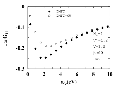
Figure 2: Imaginary part of the site-diagonal Green’s function at the $\Gamma$-point. Parameters used for DMFT+GW: $N_{k}=33$, $N_{g}=512$, $N_{h}=128$ and $N_{P}=N_{S}=64$.

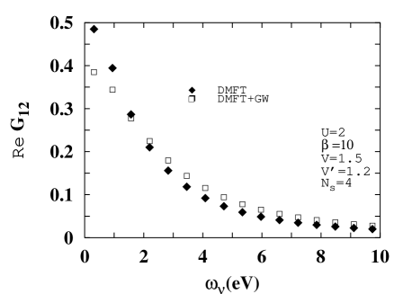
Figure 3: Real part of the site-nondiagonal Green’s function at the $\Gamma$-point. Parameters used for DMFT+GW: $N_{k}=33$, $N_{g}=512$, $N_{h}=128$ and $N_{P}=N_{S}=64$.

The GW derived polarization (Eq. 40) and screened interaction (correlated part) (Eq. 23) are displayed in Figs. (4-6) as a function of imaginary (even Matsubara) frequencies. Note that if the full polarization in Eq. 32 is required one has to correct for double counting and merely add the static impurity contribution ($P_{1}(i\omega_{m}=0)$ = -0.47). For large Matsubara energies the diagonal part approaches $2V^{\prime}$ and the non-diagonal part $2V$ as can be derived using Eq. (II.2), which is numerically confirmed. In Fig. (7) we show the screened interaction at the $\Gamma$- point along the real axis using the Pade approximation. We observe that the static value ${\rm Re}W(0)$ is merely a constant below the main excitation peak and slightly larger in the case of non-diagonal screening. However it is well-known that in the RPA the screening is overestimated at short distances. From a physical point of view this fact is easily understandable: a positive hole is surrounded or screened by a too tightly drawn electron cloud, due to the fact that exchange and correlation effects are neglected among the screening electrons.

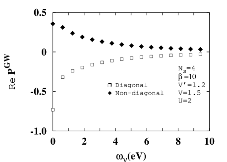
Figure 4: Real part of the polarization function at the $\Gamma$-point. The static impurity contribution is $P_{1}(i\omega_{m}=0)$ = -0.47. Parameters used for DMFT+GW: $N_{k}=33$, $N_{g}=512$, $N_{h}=128$ and $N_{P}=N_{S}=64$.

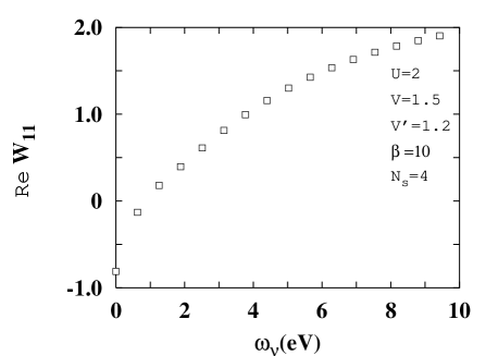
Figure 5: Real part of the site-diagonal (correlated ) screened interaction at the $\Gamma$-point. The bare Hubbard $U$ has been subtracted. The impurity screened interaction is 0.5 and the effective Hubbard ${\cal U}=0.7$. Parameters used for DMFT+GW: $N_{k}=33$, $N_{g}=512$, $N_{h}=128$ and $N_{P}=N_{S}=64$.

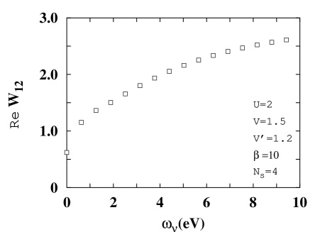
Figure 6: Real part of the site-nondiagonal screened interaction at the $\Gamma$-point. Parameters used for DMFT+GW: $N_{k}=33$, $N_{g}=512$, $N_{h}=128$ and $N_{P}=N_{S}=64$.

The self-consistent values of the impurity screened potential and the effective Hubbard on-site interaction (both defined in Eq. 30) were found to be $W(i\omega_{m}=0)=0.5$ and ${\cal U}=0.7$ respectively. Thus at self-consistency, the effective impurity problem offers an on-site interaction which is more than a factor of two smaller than the bare $U=2$. For illustration we show the charge impurity response function along the real axis in Fig. 8 derived using the effective Hubbard ${\cal U}=0.7$.

Figure 7: Real and imaginary part of the site-diagonal screened interaction at the $\Gamma$-point. We used an artificial broadening of 0.5. Parameters used for DMFT+GW: $N_{k}=33$, $N_{g}=512$, $N_{h}=128$ and $N_{P}=N_{S}=64$.

Figure 8: Real (solid line) and imaginary ( dashed line) part of the impurity response function (site 1) defined in Eq. 18 for the effective impurity. Parameters used for DMFT+GW: $N_{k}=33$, $N_{g}=512$, $N_{h}=128$ and $N_{P}=N_{S}=64$.

As discussed previously, in the single site DMFT case the solution to the impurity model is extracted using the bare Hubbard $U=2$, however in the DMFT+GW scenario the impurity model is solved with the effective (weaker) interaction ${\cal U}$. The magnitude of the impurity self-energy scales with the size of the on-site interaction making it somewhat cumbersome to compare different impurity self-energies obtained with different on-site interaction strengths. However the quantity one really should compare is the total self-energy entering the theory i.e the $U=2$ impurity DMFT single site self-energy should be compared with the full self-energy in Eq. (26). In this work a critically comparison will not be done, we briefly discuss spectral properties, which however strongly depends on the self-energy.

Prior to the discussion about spectral properties we intend to make some statements about the derived self-energies. In all the cases studied we have observed the characteristics of a metal or an insulatorrev2 : ${\rm Im}\Sigma(i\omega)<0$ increases linearly or diverges when $\omega\rightarrow 0^{+}$ respectively. Regarding the magnitude of the GW self-energy it depends strongly on the $k$-point, but in general the non-diagonal ${\rm Re}\Sigma^{GW}_{12}$ is quite large and ${\rm Im}\Sigma^{GW}_{11}$ is smaller (in comparison with relevant quantities).

It is a delicate matter to extract real frequency dynamical information from imaginary axis data. The commonly used quantum Monte Carlo impurity solver uses maximum entropy based methodsjarell . In the present work, adopting the Lanczos routine for solving the impurity problem, we used the the Pade approximation when performing the analytical continuation. For example in order to obtain the GW self-energy and spectral functions we must do an analytical continuation from the imaginary axis ($i\omega\rightarrow(\omega+i\delta)$). However, the impurity self-energy on the real axis can be extracted using the self-consistency relation in Eq. 27. The corresponding results are shown in Figs. (9, 11) (DMFT) and Fig. 10 (DMFT+GW). In the DMFT+GW scenario the impurity is solved with an effective Hubbard interaction ${\cal U}=0.7$, reflected in a substantial reduction in the magnitude. As a comparison with Fig. (9) the self-energy derived using the Pade approximation is displayed in Fig. 12.

In the metallic case the self-energy exhibits the Fermi-liquid behaviour: ${\rm Re}\Sigma(\omega)\sim(1-1/Z)\omega$ (or equivalently ${\rm Im}\Sigma(i\omega)\sim(1-1/Z)\omega$) and ${\rm Im}\Sigma(\omega)\sim-\omega^{2}$ for $\omega$ close to zero where

$$Z=(1-{\frac{\partial{\rm Re}\Sigma(\omega)}{\partial\omega)}\mid_{\omega=0}})^{-1}$$ (51)

denotes the quasiparticle renormalization factor. In the insulator case the slope of ${\rm Re}\Sigma(\omega)$ changes sign (${\rm Re}\Sigma(\omega)\rightarrow 1/\omega$ for $\omega\rightarrow 0$) and ${\rm Im}\Sigma(\omega)$ is peaked at the chemical potential and zero in the gapkramer as evident from Fig. (11).

Figure 9: Real and imaginary part of the impurity self-energy (site 1 and spin up) for a typical metal. We used an artificial broadening of 0.75. Parameters used for DMFT: $N_{k}=33$ and $N_{g}=512$.

Figure 10: Real and imaginary part of the impurity self-energy (site 1 and spin up) for a typical metal. We used an artificial broadening of 0.75. Parameters used for DMFT+GW: $N_{k}=33$, $N_{g}=512$, $N_{h}=128$ and $N_{P}=N_{S}=64$.

Figure 11: Real and imaginary part of the impurity self-energy (site 1 and spin up) for a typical insulator. We used an artificial broadening of 0.75. Parameters used for DMFT: $N_{k}=33$ and $N_{g}=512$.

Figure 12: Real and imaginary part of the impurity self-energy (site 1 and spin up) for a typical metal. Parameters used for DMFT: $N_{k}=33$ and $N_{g}=512$.

We next discuss spectral properties. In order to achieve the local density of states (LDOS) we have solved the impurity model on the real axis and then extracted ${\rm Im}G_{i\sigma}(\omega)$. As can be seen in Fig. 13, the LDOS is symmetric (half-filling $n=1$) and shows the typical Fermi metallic characteristics; a quasiparticle peak surrounding the two Hubbard bandsrev2 .

Figure 13: Local density of states for site 1 and spin up. The chemical potential corresponds to energy zero. We introduced an artificial broadening of 0.25. Parameters used for DMFT+GW: $N_{k}=33$, $N_{g}=512$, $N_{h}=128$ and $N_{P}=N_{S}=64$.

With aid of the Pade approximation and Eq. 37 we calculate the spectral functions. The zone-center spectral function is visualized in Fig. (14). A significant change of the quasiparticle peak position is clearly seen at the $\Gamma$-point, where the downward shift is around 0.4. The corresponding dispersion in the $\Gamma$-$X$ direction is displayed in Fig. 16. Interestingly when only one iteration with the GW kernel is performed on top of a self-consistent DMFT calculation, the dispersion essentially coincide with the DMFT one.

Figure 14: Spectral function at the $\Gamma$-point. The chemical potential corresponds to energy zero. The solid line corresponds to the DMFT+GW case and the dashed line to the DMFT case. We used an artificial broadening of 0.5. Parameters used: $N_{k}=33$, $N_{g}=512$, $N_{h}=128$ and $N_{P}=N_{S}=64$.

Figure 15: Spectral function at the $X$-point. The chemical potential corresponds to energy zero. The solid line corresponds to the DMFT+GW case and the dashed line to the DMFT case. We used an artificial broadening of 0.5. Parameters used: $N_{k}=33$, $N_{g}=512$, $N_{h}=128$ and $N_{P}=N_{S}=64$.

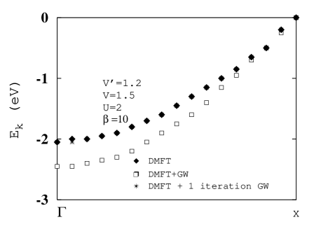
Figure 16: Quasiparticle dispersion in the $\Gamma$-$X$ direction. Parameters used: $N_{k}=33$, $N_{g}=512$, $N_{h}=128$ and $N_{P}=N_{S}=64$.

To obtain a notable effect with the GW kernel, one has in general to include the long-range part of the bare Coulomb potential and consider nearest ($V$) and next nearest neighbors interaction ($V^{\prime}$). For example the parameter-set $V=V^{\prime}=0$ gives a quasiparticle peak position shifted only by 0.1 compared to the DMFT situation (the shift is 0.4 with $V=1.5,V^{\prime}=1.2$) which is realized from Fig. 17. If one compare the lattice Green’s function in Fig. 2 and Fig. 18, it is obvious that DMFT and DMFT+GW with the long-range part excluded ($V=V^{\prime}=0$) are quite similar.

Figure 17: Spectral function (DMFT+GW) at the $\Gamma$-point . The chemical potential corresponds to energy zero. The solid line corresponds to $V=1.5,V^{\prime}=1.2$ and the dashed line to $V=V^{\prime}=0$. We used an artificial broadening of 0.5. Parameters used: $N_{k}=33$, $N_{g}=512$, $N_{h}=128$ and $N_{P}=N_{S}=64$.

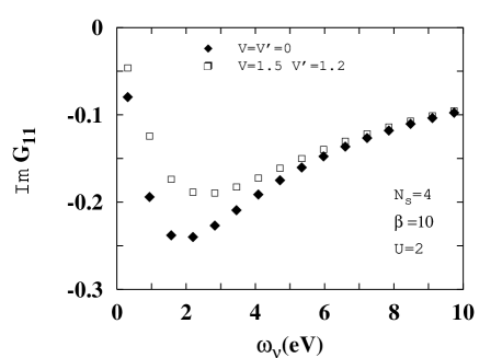
Figure 18: Imaginary part of the site-diagonal Green’s function (DMFT+GW) at the $\Gamma$-point. Parameters used for DMFT+GW: $N_{k}=33$, $N_{g}=512$, $N_{h}=128$ and $N_{P}=N_{S}=64$.

Next we briefly consider a 1D insulator using the parameter-set $U=14$, $V=3$ and $V^{\prime}=2$. In contrast to the metal case the screening is less effective giving the self-consistent impurity screened interaction to be 13.7 and the effective Hubbard ${\cal U}=13.9$. The similarities between the screened and bare interactions indicate that the off-site hopping parameters $V$ and $V^{\prime}$ are too small to give rise to a notable effect, which is indeed confirmed by the spectral function shown in Fig. 19. Furthermore it is worth to note that in the strong insulator case the imaginary part of the (site-diagonal) impurity self-energy is diverging for small $i\omega$ ($\Sigma(i\omega)\rightarrow 1/i\omega$), making at least the significance of the diagonal GW self-energy negligible. However non-diagonal GW contributions can influence the spectral functions.

Figure 19: Spectral function at the $\Gamma$-point. The chemical potential corresponds to energy zero. The solid line corresponds to the DMFT+GW case and the dashed line to the DMFT case. We used an artificial broadening of 0.5. Parameters used: $N_{k}=33$, $N_{g}=512$, $N_{h}=128$ and $N_{P}=N_{S}=64$.

III.2 2D square lattice

The bandwidth of the 2D square lattice is 8 and we have chosen $U=4$ and $U=18$ as prototypes for a metal and an insulator respectively. As in 1D $N_{s}=4$ is sufficient. We will first discuss the metal case. The reasoning and organization follows closely the setup in the previous section. We have chosen the parameters $V=1.5$ and $V^{\prime}=0.75$ in the metal case $U=4$. In Figs. (20-21) the lattice Green’s function are shown

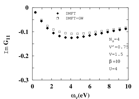
Figure 20: Imaginary part of the site-diagonal Green’s function at the $\Gamma$-point. Parameters used for DMFT+GW: $N_{k}=169$, $N_{g}=512$, $N_{h}=128$ and $N_{P}=N_{S}=64$.

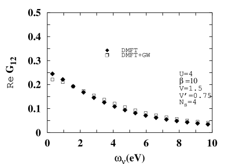
Figure 21: Real part of the site-nondiagonal Green’s function at the $\Gamma$-point. Parameters used for DMFT+GW: $N_{k}=169$, $N_{g}=512$, $N_{h}=128$ and $N_{P}=N_{S}=64$.

whereas the corresponding polarization and screened interaction are displayed in Figs. (22-24). At self-consistency the impurity screened interaction is 0.7 and the effective Hubbard ${\cal U}=2.4$, strongly reduced compared to the bare values. We stress that the amount of screening that are taking place is in general dependent of the non-locality parameters $V$ and $V^{\prime}$, which in this work is chosen arbitrarily. In 2D the large $i\omega$ limit is numerically satisfied: the diagonal part approaches $4V^{\prime}$ and the non-diagonal part $4V$ respectively. It is worth mention that the overall magnitude of the polarization function $P^{GW}(i\omega)$ decreases for increasing $U$. As a consequence, the overall magnitude of the correlated part of the screened interaction $W^{c}(i\omega)$ increases for increasing $U$. As a comparison to the 1D case, the screened interaction on real axis at the $\Gamma$-point is shown in Fig. 25.

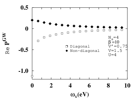
Figure 22: Real part of the polarization function at the $\Gamma$-point. The static impurity contribution is $P_{1}(i\omega_{m}=0)$ = -1.1. Parameters used for DMFT+GW: $N_{k}=169$, $N_{g}=512$, $N_{h}=128$ and $N_{P}=N_{S}=64$.

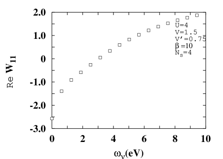
Figure 23: Real part of the site-diagonal (correlated) screened interaction at the $\Gamma$-point. The bare Hubbard $U$ has been subtracted. Parameters used for DMFT+GW: $N_{k}=169$, $N_{g}=512$, $N_{h}=128$ and $N_{P}=N_{S}=64$.

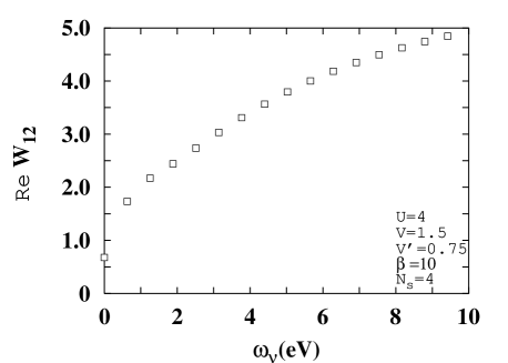
Figure 24: Real part of the site-nondiagonal screened interaction at the $\Gamma$-point. Parameters used for DMFT+GW: $N_{k}=169$, $N_{g}=512$, $N_{h}=128$ and $N_{P}=N_{S}=64$.

Figure 25: Real and imaginary part of the site-diagonal screened interaction at the $\Gamma$-point. We used an artificial broadening of 0.5. Parameters used for DMFT+GW: $N_{k}=169$, $N_{g}=512$, $N_{h}=128$ and $N_{P}=N_{S}=64$.

As an illustration we display in Fig. (26) the $GW$ self-energy, which clearly exhibits Fermi-liquid characteristics, derived using Eq. 44.

Figure 26: Real and imaginary part of the GW self-energy including the double counting term (site 1 and spin up) for a typical metal. We used an artificial broadening of 0.5. Parameters used for DMFT+GW: $N_{k}=33$, $N_{g}=512$, $N_{h}=128$ and $N_{P}=N_{S}=64$.

The metallic LDOS and a typical quasiparticle spectral function are shown in Figs. (27-28). The downward shift of the quasiparticle position is consistent with the scenario observed in the 1D case.

Figure 27: Local density of states for site 1 and spin up. The chemical potential corresponds to energy zero. We introduced an artificial broadening of 0.25. Parameters used for DMFT+GW: $N_{k}=169$, $N_{g}=512$, $N_{h}=128$ and $N_{P}=N_{S}=64$.

Figure 28: Spectral function at the $\Gamma$-point. The chemical potential corresponds to energy zero. The solid line corresponds to the DMFT+GW case and the dashed line to the DMFT case. We used an artificial broadening of 0.5. Parameters used: $N_{k}=169$, $N_{g}=512$, $N_{h}=128$ and $N_{P}=N_{S}=64$.

Let us finally consider the strong insulator case $U=18$. We have chosen the parameters $V=4$ and $V^{\prime}=3$ which can be considered as a substantial off-site interaction, however there exists no large difference in the DMFT Green’s function compared to the DMFT+GW one (see Figs. (29-30)). The impurity screening is found to $W(i\omega_{m}=0)=16.9$ the effective Hubbard ${\cal U}=17.1$, implying a reduced bandgap.

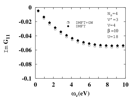
Figure 29: Imaginary part of the site-diagonal Green’s function at the $\Gamma$-point. Parameters used for DMFT+GW: $N_{k}=169$, $N_{g}=512$, $N_{h}=128$ and $N_{P}=N_{S}=64$.

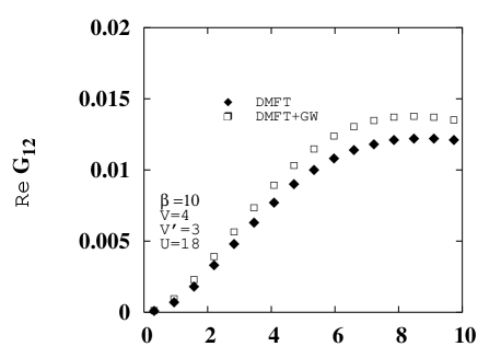
Figure 30: Real part of the site-nondiagonal Green’s function at the $\Gamma$-point. Parameters used for DMFT+GW: $N_{k}=169$, $N_{g}=512$, $N_{h}=128$ and $N_{P}=N_{S}=64$.

The corresponding spectral function is shown in Fig. (31). We note that in the strong insulator case the Hubbard gap ($\sim{\cal U}$) is indeed somewhat reduced due to the inclusion of the GW self-energy.

Figure 31: Spectral function at the $\Gamma$-point. The chemical potential corresponds to energy zero. The solid line corresponds to the DMFT+GW case and the dashed line to the DMFT case. We used an artificial broadening of 0.5. Parameters used: $N_{k}=169$, $N_{g}=512$, $N_{h}=128$ and $N_{P}=N_{S}=64$.

IV Concluding remarks

In the present study a full self-consistency is performed, including the non-local GW self-energy, in the local single site DMFT approach and the applicability of the method is tested for a model system. Eventually at self-consistency the full self-energy and polarization operator are obtained, from which e.g the full screened interaction is accessible. Far from the metal-insulator transition the combination of the GW method and the single site DMFT is from a numerical point of view fast and stable, even when a simple linear mixing scheme is utilized. Changes with respect to DMFT are in some cases substantial, and are related to the long-rangeness of the GW kernel, specified by two hopping parameters.

Next we will study the 2D metal-insulator transition as well as doping away from half-filling.

V Acknowledgments

We greatly acknowledge discussions with Ferdi Aryasetiawan, Silke Biermann and Roger Bengtsson.

References

- (1) P. Hohenberg and W. Kohn, Phys. Rev. 136, B864 (1964); W. Kohn and L. Sham, Phys. Rev. 140, A1133 (1965).
- (2) R. Jones and O. Gunnarsson, Rev. Mod. Phys. 61, 689 (1989).
- (3) L. Hedin, Phys. Rev. 139, A796, (1965).
- (4) F. Aryasetiawan and O. Gunnarsson, Rep. Prog. Phys. 61, 237, (1998).
- (5) G. Onida, L. Reining and A. Rubio, Rev. Mod. Phys. 74, 601 (2002).
- (6) V. I. Anisimov, J. Zaanen and O. K. Andersen, Phys. Rev. B 44, 943 (1991).
- (7) V. I. Anisimov, I. V. Solovyev, M. A. Korotin, M. T. Czyzyk and G. A. Zawatzky, Phys. Rev. B 48, 16929 (1993).
- (8) A. I. Lichtenstein, J. Zaanen and V. I. Anisimov, Phys. Rev. B 52, R5467 (1995).
- (9) For a review see: V. I. Anisimov, F. Aryasetiawan and A. I. Lichtenstein, J. Phys. Cond. Matter 9, 767, (1997).
- (10) A. I. Lichtenstein and M. Katsnelson, Phys. Rev. B 57, 6884 (1998).
- (11) A. I. Lichtenstein, M. Katsnelson and G. Kotliar, Phys. Rev. Lett 87, 067205 (2001).
- (12) For a review see: A. Georges, G. Kotliar, W. Krauth and M. Rozenberg, Rev. Mod. Phys. 68, 13 (1996).
- (13) T. Pruschke et al., Adv. Phys. 42, 187 (1995).
- (14) M. Imada, A. Fujimori and Y. Tokura, Rev. Mod. Phys. 70, 1039 (1998).
- (15) For a review see: T. Maier, M. Jarell, T. Pruschke and M. H. Hettler, cond-mat/0404055 (unpublished).
- (16) T. Maier, M. Jarell, T. Pruschke and J. Keller, Eur. Phys. J. B 13, 613 (2000); M. H. Hettler, A. N. Tahvildar-Zadeh, M. Jarell, T. Pruschke and H. R. Krishnamurthy, Phys. Rev. B 58, R7475 (1998); M. H. Hettler, M. Mukherjee, M. Jarell and H. R. Krishnamurthy, Phys. Rev. B 61, 12739 (2000) .
- (17) A. I. Lichtenstein and and M. I. Katsnelson, Phys. Rev. B 62, R9283 (2000).
- (18) G. Kotliar, S. Y. Savrasov, G. Palsson and G. Biroli, Phys. Rev. Lett 87, 186401 (2001).
- (19) G. Biroli and G. Kotliar, Phys. Rev. B 65, 155112 (2002).
- (20) G. Biroli, O. Parcollet and G. Kotliar, cond-mat/0307587 (unpublished); O. Parcollet, G. Biroli and G. Kotliar, Phys. Rev. Lett 92, 226402 (2004).
- (21) Q. Si and J. L. Smith, Phys. Rev. Lett 77, 3391 (1996).
- (22) H. Kajueter, PhD thesis, Rutgers University, (1996).
- (23) A. M. Sengupta and G. Kotliar, Phys. Rev. B 52, 10295 (1995).
- (24) E. C. Carter and A. J. Schofield, Phys. Rev. B 70, 045107 (2004).
- (25) S. Florens and A. Georges, Phys. Rev. B 66, 165111 (2002).
- (26) K. Haule, S. Kirchner, J. Kroha and P. W lfe, Phys. Rev. B 64, 155111 (2001).
- (27) For a review see: M. Jarell and J. E. Gubernatis, Physics Reports, 269, 133 (1996).
- (28) M. Caffarel and W. Krauth, Phys. Rev. Lett 72, 1545 (1994).
- (29) V. Oudovenko, K. Haule, S. Y. Savrasov, D. Villani and G. Kotliar, cond-mat/0403093 (unpublished).
- (30) V. I. Anisimov, A. I. Poteryaev, M. A. Korotin, A. O. Anokhin and G. Kotliar, J. Phys. Cond. Matter 35, 7359, (1997).
- (31) For a review see: Strong Coulomb correlations in electronic structure calculations , edited by V. I. Anisimov, Advances in Condensed Material Science (Gordon and Breach, New York, 2001); G. Kotliar and S. Savrasov, cond-mat/0208241 (unpublished).
- (32) O. Gunnarsson, O. K. Andersen, O. Jepsen and J. Zaanen, Phys. Rev. B 39, 1708 (1989).
- (33) M. S. Hybertsen, M. Schlüter and N. E. Christensen, Phys. Rev. B 39, 9028 (1989).
- (34) A. K. McMahan, R. M. Martin and S. Satpathy, Phys. Rev. B 38, 6650 (1988).
- (35) S. Y. Savrasov, G. Kotliar and E. Abrahams, Nature, 410, 793 (2001).
- (36) A. Poteryaev, A. I. Lichtenstein, and G. Kotliar, Phys. Rev. Lett 92, 176403 (2004).
- (37) E. Pavarini, S. Biermann, A. Poteryaev, A. I. Lichtenstein, A. Georges and O. K. Andersen, Phys. Rev. Lett 92, 176403 (2004).
- (38) D. Pines, Elementary Excitations in Solids (Benjamin, New York), (1963).
- (39) W. Ku and A. G. Equiluz, Phys. Rev. Lett 89, 126401 (2002).
- (40) M. L. Tiago, S. Ismail-Beigi, S. G. Louie, cond-mat/0307181 (unpublished).
- (41) S. V. Faleev, M. van Schilfgaarde and T. Kotani, cond-mat/0310677 (unpublished).
- (42) F. Aryasetiawan, T. Miyake and K. Terakura, Phys. Rev. Lett 88, 166401 (2002).
- (43) P. Garcia-Gonzalez and R. W. Godby, Phys. Rev. B 63, 75112 (2001).
- (44) B. Holm and U. von Barth, Phys. Rev. B 57, 2108 (1998).
- (45) W. D. Schone and A. G. Equiluz, Phys. Rev. Lett 81, 1662 (1998).
- (46) H. J. de Groot, P. A. Bobbert and W. Haeringen, Phys. Rev. B 52, 11000 (1995.
- (47) E. L. Shirley, Phys. Rev. B 54, 7758 (1996).
- (48) G. Baym and L. P. Kadanoff, Phys. Rev. 124, 287 (1961); G. Baym, Phys. Rev. 127, 1662 (1962);
- (49) S. Biermann, F. Aryasetiawan and A. Georges, Phys. Rev. Lett 90, 086402 (2003).
- (50) P. Sun and G. Kotliar, Phys. Rev. B 66, 085120 (2002).
- (51) P. Sun and G. Kotliar, Phys. Rev. Lett 92, 196402 (2004).
- (52) M. Fleck, A. I. Lichtenstein and A. M. Olés, Phys. Rev. B 64, 134528 (2001).
- (53) In the case of a one-dimensional (1D) lattice: real space tranlation vector , basis vectors and , reciprocal vector . The lattice has 2 symmetry operations. In the case of a two-dimensional (2D) square lattice: real space tranlation vectors and , basis vectors and , reciprocal vectors and . The lattice has 8 symmetry operations.
- (54) The 2D case is described, however to consider the 1D case the modifications are minor. The hopping matrix have non-diagonal elements in the chain case.
- (55) M. Capone, M. Civelli, S. S. Kancharla, C. Castellani and G. Kotliar, Phys. Rev. B 69, 195105 (2004).
-
(56)
Due to the defintion of the contribution
is implicitely included in . - (57) Symmetry for and in the 2D case: diagonal elements for all . Non-diagonal elements () if () even and if () odd. Further , where lies in the IBZ, because .
- (58) The polarization operator obeys . The self-energy operator obeys .
- (59) M. Jarell and J. E. Gubernatis, Physics Reports 269 133-195 (1996).
-
(60)
The Kramer-Kronig (KK) relations can be written as
which are very important in connecting the real and imaginary part of a given complex function. With the knowledge of the self-energy on the whole real axis on can perform an analytical continuation to the imaginary axis(52)
for any in the upper half-plane. It is readily shown that and if symmetric around . Furthermore it can be shown that the slopes of and are equal for small and if the spectral function has zero amplitude at the chemical potential .