Entropy production and Pesin-like identity at the onset of chaos

Abstract

Asymptotically entropy of chaotic systems increases linearly and the sensitivity to initial conditions is exponential with time: these two behaviors are related. Such relationship is the analogous of and under specific conditions has been shown to coincide with the Pesin identity. Numerical evidences support the proposal that the statistical formalism can be extended to the edge of chaos by using a specific generalization of the exponential and of the Boltzmann-Gibbs entropy. We extend this picture and a Pesin-like identity to a wide class of deformed entropies and exponentials using the logistic map as a test case. The physical criterion of finite-entropy growth strongly restricts the suitable entropies. The nature and characteristics of this generalization are clarified.

It has been suggested that exponential and power-law sensitivity to initial conditions of chaotic systems could be unified through the concept of generalized exponential leading to the definition of generalized Lyapunov exponents Tsallis:1997 : the sensitivity $\xi\equiv\lim_{\Delta x(0)\to 0}\Delta x(t)/\Delta x(0)$ grows asymptotically as a generalized exponential $\widetilde{\exp}(\lambda t)$, where $\widetilde{\exp}(x)=\exp_{q}(x)\equiv[1+(1-q)x]^{1/(1-q)}$; the exponential behavior for the chaotic regime is recovered for $q\to 1$: $\lim_{q\to 1}\exp_{q}(\lambda_{q}t)=\exp(\lambda t)$.

The Kolmogorov-Sinai (K-S) entropy is defined as the time-averaged production rate of Shannon entropy over the joint probability for the trajectory to pass through a given sequence of steps in phase space with appropriate coding of the sequence and limit of the volume that characterize the steps. The K-S definition for most systems is not easily amenable to numerical evaluation and not directly equivalent to the usual thermal or statistical entropy. The connection between the K-S entropy production rate and the statistical entropy of fully chaotic systems and, in particular, of the three successive stages in the entropy time evolution is discussed in Ref. Latora:1999prl . After a first initial-condition-dependent stage, the entropy grows linearly in the limit of infinitely fine coarse graining: this is the characteristic asymptotic regime. The last stage depends on the practical limitation of the coarse graining.

Since this statistical definition of entropy production rate, where an ensemble of initial conditions confined to a small region is let evolve, appears to be relevant to thermal processes and practically coincides with the K-S entropy in chaotic regimes Latora:1999prl , we use it and call from now one K-S entropy $K$, even if it is in principle different.

The rate of loss of information relevant for the above-mentioned systems, which include both full-chaotic and edge-of-chaos cases, should be suitably generalized. In fact at the edge of chaos this picture appears to be recovered with the generalized entropic form proposed by Tsallis Tsallis:1987eu $S_{q}=(1-\sum_{i=1}^{W}p_{i}^{q})/(q-1)$, which grows linearly for a specific value of the entropic parameter $q=q_{\mathrm{sens}}=0.2445$ for the logistic map: $\lim_{t\to\infty}\lim_{L\to 0}S_{q}(t)/t=K_{q}$, where $S_{q}$ reduces to $-\sum_{i=1}^{W}p_{i}\log p_{i}$ in the limit $q\to 1$ $p_{i}$ being the fraction of the ensemble found in the $i$-th cell of linear size $L$. The same exponent describes the asymptotic power-law sensitivity to initial conditions Latora:1999vk .

Finally, it has been also conjectured that the relationship between the asymptotic entropy-production rate $K$ and the Lyapunov exponent $\lambda$ for chaotic systems (Pesin-like identity) can be extended to $K_{q}=\lambda_{q}$ Tsallis:1997 .

Numerical evidences supporting this framework with the entropic form $S_{q}$ have been found for the logistic Tsallis:1997 and generalized logistic-like maps Tsallis:1997cl . Ref. Lyra:1998wz gives scaling arguments that relate the asymptotic power-law behavior of the sensitivity to the fractal scaling properties of the attractor. Finite-size scaling relates numerically the entropic parameter $q$ to the power-law convergence to the box measure of the attractor from initial conditions uniformly spread over phase space deMoura:2000 ; Borges:2002 . The linear behavior of the generalized entropy for specific choices of $q$ has been observed for two families of one-dimensional dissipative maps Tirnakli:2001 .

Renormalization-group methods have been recently used Baldovin:2002a ; Baldovin:2002b to demonstrate that the asymptotic (large $t$) behavior of the sensitivity to initial conditions in the logistic and generalized logistic maps is bounded by a specific power-law whose exponent could be determined analytically for initial conditions on the attractor. Again for evolution on the attractor the connection between entropy and sensitivity has been studied analytically and numerically, validating a Pesin-like identity for Tsallis’ entropic form Baldovin:2004 .

Sensitivity and entropy production have been studied in one-dimensional dissipative maps using ensemble-averaged initial conditions chosen uniformly over the interval embedding the attractor Ananos:2004a : the statistical picture, i.e., the relation between sensitivity and entropy exponents and the Pesin-like identity, has been confirmed even if with a different $q=q_{\mathrm{sens}}^{\mathrm{ave}}=0.35$ Ananos:2004a . Indeed the ensemble-averaged initial conditions appear more relevant for the connection between ergodicity and chaos and for practical experimental settings. The same analysis has been repeated for two symplectic standard maps Ananos:2004b .

The main objective of the present work is to demonstrate the more general validity of the above-described picture and, specifically, of the extended Pesin-like identity and of the physical criterion of finite-entropy production per unit time (linear growth), which strongly selects appropriate entropies and fixes their parameters. For this purpose we use the coherent statistical framework arising from the following two-parameter family Mittal ; Taneja1 ; Borges1 ; Kaniadakis:2004nx ; Kaniadakis:2004ri ; Kaniadakis:2004td of logarithms

$$\widetilde{\log}(\xi)\equiv\frac{\xi^{\alpha}-\xi^{-\beta}}{\alpha+\beta}\quad,$$ (1)

where $\alpha$ ($\beta$) characterizes the large (small) argument asymptotic behavior; in particular, $\widetilde{\exp}(\lambda t)\equiv\widetilde{\log}^{-1}(\lambda t)\sim(\lambda t)^{1/\alpha}$ for large $t$. The requirements that the logarithm be an increasing function, therefore invertible, with negative concavity (the related entropy is stable), and that the exponential be normalizable for negative arguments (see Ref. Naudts1 for a discussion of the criteria) select $0\leq\alpha\leq 1$ and $0\leq\beta<1$ Kaniadakis:2004td ; solutions with negative $\alpha$ and $\beta$ are duplicate, since the family (1) possesses the symmetry $\alpha\leftrightarrow-\beta$. We have studied the entire class of logarithms and exponentials and will show results for the following four interesting one-parameter cases:

(1) the original Tsallis proposal Tsallis:1987eu : $\alpha=1-q$ and $\beta=0$;

(2) the Abe logarithm: $q_{A}=1/(1+\alpha)$ and $\beta=\alpha/(1+\alpha)$, named after the entropy introduced by Abe Abe:1997qg , which possesses the symmetry $q_{A}\to 1/q_{A}$;

(3) the Kaniadakis logarithm: $\alpha=\beta=\kappa$, which shares the same symmetry group of the relativistic momentum transformation and has applications in cosmic-ray and plasma physics Kaniadakis:2001nl ; Kaniadakis:2002sr ; Kaniadakis:2005zk ;

(4) in addition we have considered a sample spanning the entire class (values of $\beta$): in this letter we show results for the choice $\alpha=2\beta=2\gamma$, which we label $\gamma$ logarithm .

We study the sensitivity to initial conditions and the entropy production in the logistic map $x_{i+1}=1-\mu x^{2}_{i}$, at the infinite bifurcation point $\mu_{\infty}=1.401155189$. If the sensitivity follows a deformed exponential $\xi(t)=\widetilde{\exp}(\lambda t)$, analogously to the chaotic regime when $\xi(t)\sim\exp(\lambda t)$, the corresponding deformed logarithm of $\xi$ should yield a straight line $\widetilde{\log}(\xi(t))=\widetilde{\log}(\widetilde{\exp}(\lambda t))=\lambda t$.

The sensitivity has been calculated using the exact formula for the logistic map $\xi(t)=(2\mu)^{t}\prod_{i=0}^{t-1}|x_{i}|$ for $1\leq t\leq 80$, and the generalized logarithm $\widetilde{\log}(\xi)$ has been uniformly averaged over the entire interval $-1<x_{0}<1$ by randomly choosing $4\times 10^{7}$ initial conditions. The averaging over initial conditions, indicated by $\langle\cdots\rangle$, is appropriate for a comparison with the entropy production.

Guided by Ref. Ananos:2004a , for each of several generalized logarithms, $\langle\widetilde{\log}(\xi(t))\rangle$ has been fitted to a quadratic function for $1\leq t\leq 80$ and $\alpha$ has been chosen such that the coefficient of the quadratic term be zero; in fact $\widetilde{\log}(\xi)$ linear in $t$ means that the sensitivity $\xi$ behaves as $\widetilde{\exp}(\lambda t)$: we label this value $\alpha^{\mathrm{av}}_{\mathrm{sens}}$.

In fact, the exponent obtained with this procedure has been denoted $q_{\mathrm{sens}}^{\mathrm{av}}$ in the case of Tsallis’ entropy Ananos:2004a to mark the difference with the exponent $q_{\mathrm{sens}}$ obtained by choosing an initial condition at the fixed point of the map $x_{0}=0$ Baldovin:2004 .

Table 1 reports the values of $\alpha^{\mathrm{av}}_{\mathrm{sens}}$ corresponding to four different choices of the logarithm with the shown statistical errors calculated by repeating the fitting procedure for sub-samples of the $4\times 10^{7}$ initial conditions; in addition we estimate a systematic error of about $0.004$ by fitting over different ranges of $t$. The exponent we find using Tsallis’ formulation $\alpha^{\mathrm{av}}_{\mathrm{sens}}=0.644\pm 0.002$ is consistent within the errors with the value quoted in Ref. Ananos:2004a $q^{\mathrm{av}}_{\mathrm{sens}}=1-\alpha^{\mathrm{av}}_{\mathrm{sens}}\approx 0.36$. The values of $\alpha^{\mathrm{av}}_{\mathrm{sens}}$ are within $\pm 1\%$: taking into account the systematic error arising from the inclusion in the global fitting of small values of $\xi$, for which the different formulations have not yet reached their common asymptotic behavior (at least at the level of 1%), it can be estimated $\alpha^{\mathrm{av}}_{\mathrm{sens}}=0.650\pm 0.005$.

Table 1: For each of the generalized logarithms listed in the first row the following quantities are given: the exponents of the leading-power behavior for large- ($\alpha$) and small- ($\beta$) arguments according to Eq. (1); the experimental generalized Lyapunov exponents $\lambda$ (see Fig. 1) and the experimental rates of entropy growth $K$ (see Fig. 2), which verify the generalized Pesin-like identity $K=\lambda$; the asymptotic ($\nu_{\mathrm{eff}}=\infty$) and corrected ($\nu_{\mathrm{eff}}=20$) theoretical predictions for $K_{\beta}$ relative to $K_{0}$ ($\beta=0$ or Tsallis’ case) from Eq. (3), and the corresponding experimental values. Statistical errors are shown.

	Tsallis	$\gamma$	Abe	Kaniadakis
$\alpha$	$0.644\pm 0.002\$	$0.656\pm 0.002$	$0.657\pm 0.002$	$0.653\pm 0.002$
$\beta$	0	0.328	0.396	0.653
$\lambda$	$\mathbf{0.271}\pm 0.003$	$\mathbf{0.198}\pm 0.002$	$\mathbf{0.185}\pm 0.002$	$\mathbf{0.148}\pm 0.001$
K	$\mathbf{0.267}\pm 0.003$	$\mathbf{0.197}\pm 0.002$	$\mathbf{0.186}\pm 0.002$	$\mathbf{0.152}\pm 0.002$
$\left(K/K_{0}\right)_{\mathrm{Asymp}}$	1	0.667	0.623	0.500
$\left(K/K_{0}\right)_{\mathrm{Theory}}$	1	0.736	0.695	0.571
$\left(K/K_{0}\right)_{\mathrm{Experim}}$	1	$0.738\pm 0.004$	$0.697\pm 0.004$	$0.569\pm 0.004$

Figure 1 shows the straight-line behavior of $\widetilde{\log}(\xi)$ for all four formulations when $\alpha=\alpha^{\mathrm{av}}_{\mathrm{sens}}$: the corresponding slopes $\lambda$ (generalized Lyapunov exponents) are reported in Table 1 with their statistical errors; a systematic error of about 0.003 has been estimated by different choices of the range of $t$. While the values of $\alpha$ are consistent with a universal exponent independent of the particular deformation, the slope $\lambda$ strongly depends on the choice of the logarithm.

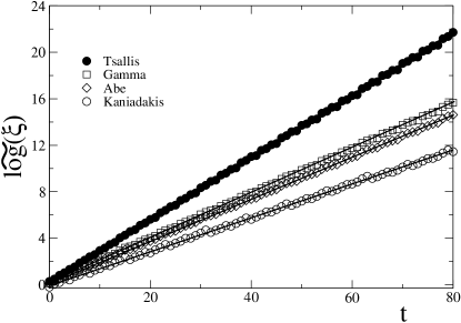
Figure 1: Generalized logarithms $\widetilde{\log}(\xi)$, see Eq. (1), of the sensitivity to initial conditions averaged over $4\times 10^{7}$ uniformly distributed initial conditions as function of time. From top to bottom: Tsallis’, $\gamma$, Abe’s, and Kaniadakis’ logarithms. The linear rising behavior has been obtained with the asymptotic powers $\alpha$ shown in Table 1; the corresponding generalized Lyapunov exponents $\lambda$ can also be read in Table 1.

The entropy has been calculated by dividing the interval $(-1,1)$ in $W=10^{5}$ equal-size boxes, putting at the initial time $N=10^{6}$ copies of the system with an uniform random distribution within one box, and then letting the systems evolve according to the map. At each time $p_{i}(t)\equiv n_{i}(t)/N$, where $n_{i}(t)$ is the number of systems found in the $i$-th box at time $t$, the entropy of the ensemble is

$$S(t)\equiv\left\langle\sum_{i=1}^{W}p_{i}(t)\widetilde{\log}(\frac{1}{p_{i}(t)})\right\rangle=\left\langle\sum_{i=1}^{W}\frac{p_{i}^{1-\alpha}(t)-p_{i}^{1+\beta}(t)}{\alpha+\beta}\right\rangle$$ (2)

where $\langle\cdots\rangle$ is an average over $2\times 10^{4}$ experiments, each one starting from one box randomly chosen among the $W$ boxes. The choice of the entropic form (2) is fundamental for a coherent statistical picture: the usual constrained variation of the entropy in Eq. (2) respect to $p_{i}$ yields as distribution the deformed exponential $\widetilde{\exp}(x)$ whose inverse is indeed the logarithm appearing in Eq. (1) Kaniadakis:2004td .

Analogously to the strong chaotic case, where an exponential sensitivity ($\alpha=\beta=0$) is associated to a linear rising Shannon entropy, which is defined in terms of the usual logarithm ($\alpha=\beta=0$), and consistently with the conjecture in Ref. Tsallis:1997 , the same values $\alpha$ and $\beta$ of the sensitivity are used in Eq. (2): Fig. 2 shows that this choice leads to entropies that grow also linearly. We have also verified that this linear behavior is lost for values of the exponent $\alpha$ different from $\alpha^{\mathrm{av}}_{\mathrm{sens}}$, confirming for the whole class (2) what was already known for the $q$-logarithm Tsallis:1997 ; Ananos:2004a .

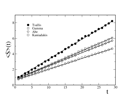
Figure 2: Entropy as function of time, averaged over $2\times 10^{4}$ experiments, each one with an ensemble of $10^{6}$ points over a grid of $10^{5}$ boxes. The entropies belong to the class of Eq. (2) and are defined with exactly the same exponents $\alpha$ and $\beta$ used for the sensitivities; as in Fig. 1, the curves show Tsallis’, $\gamma$, Abe’s, and Kaniadakis’ entropies from top to bottom. Straight lines are guides to the eyes. The resulting rates of growth of entropy $K$ can be read in Table 1.

In Table 1 we report the rate of growth of several entropies $K_{\beta}=S_{\beta}(t)/t$; the statistical errors have been again estimated by sub-sampling the experiments. While this rate $K$ depends on the choice of the entropy, the Pesin-like identity holds for each given deformation: $K_{\beta}=\lambda_{\beta}$.

There exists an intuitive explanation of the dependence of the value of $K$ on $\beta$, i.e., on the choice of the deformation. If the ensemble at time $t$ is spread approximately uniformly over $\nu$ boxes, while the other $(W-\nu)$ boxes are practically empty the entropy is $S(t)\approx\widetilde{\log}(\nu(t))\sim[\nu^{\alpha}(t)-\nu^{-\beta}(t)]/(\alpha+\beta)$, being $\nu$ an effective average number of occupied boxes. Since the exponent $\alpha$ is a property of the map, and practically independent of the entropic form, and choosing the rate of growth of Tsallis’ entropy $K_{0}$, which corresponds to $\beta=0$, as reference, the dependence of $K_{\beta}$ on the choice of $\beta$ results:

$$\frac{K_{\beta}}{K_{0}}=\left(1+\frac{\beta}{\alpha}\right)^{-1}\times\frac{1-\nu^{-\alpha-\beta}}{1-\nu^{-\alpha}}\quad.$$ (3)

The first factor is the asymptotic $(\nu\gg 1)$ ratio that depends only on $\alpha$ and $\beta$, while the second factor gives the leading finite size correction. The last three lines of Table 1 compare the asymptotic and corrected theoretical predictions of Eq. (3) with the numerical experiment: this intuitive picture appears to hold with a 10% discrepancy between the asymptotic value and the corrected one which in turns reproduces accurately the experimental results with an effective number of occupied boxes $\nu\approx 20$. This result is clearly not restricted to the four representative cases explicitly shown.

In summary, numerical evidence corroborates and extends Tsallis’ conjecture that, analogously to strongly chaotic systems, also weak chaotic systems can be described by an appropriate statistical formalism. Such extended formalisms should verify precise requirements (concavity, Lesche stability Scarfone:2004ls , and finite-entropy production per unit time) to both correctly describe chaotic systems and provide a coherent statistical framework: especially the last criterion restricts the entropic forms to the ones with the correct asymptotic behavior. These results have been exemplified in a specific two-parameter class that meets all these requirements: it is the simplest power-law form describing small and large probability behavior and includes Tsallis’s seminal proposal. More specifically, the logistic map shows

(i) a power-low sensitivity to initial condition with a specific exponent $\xi\sim t^{1/\alpha}$, where $\alpha=0.650\pm 0.005$; this sensitivity can be described by deformed exponentials with the same asymptotic behavior $\xi(t)=\widetilde{\exp}(\lambda t)$ (see Fig. 1 for examples);

(ii) a constant asymptotic entropy production rate (see Fig. 2) for trace-form entropies with a specific power-behavior $p^{1-\alpha}$ in the limit of small probabilities only when the exponent $\alpha$ is the same appearing in the sensitivity;

(iii) the asymptotic exponent $\alpha$ is related to parameters of known entropies: for instance $\alpha=1-q$, where $q$ is the entropic index of Tsallis’ thermodynamics Tsallis:1987eu ; $\alpha=1/q_{A}-1$, where $q_{A}$ appears in a generalization of Abe’s entropy Abe:1997qg ; $\alpha=\kappa$, where $\kappa$ is the parameter in Kaniadakis’ statistics Kaniadakis:2001nl ; Kaniadakis:2002sr ; Kaniadakis:2005zk ;

(iv) a generalized Pesin-like identity holds $S_{\beta}/t\to K_{\beta}=\lambda_{\beta}$ for each choice of entropy and corresponding exponential in the class, even if the value of $K_{\beta}=\lambda_{\beta}$ depends on the specific entropy (or choice of $\beta$) and it is not characteristic of the map as it is $\alpha$ (see Table 1 for examples);

(v) the ratios between the entropy production rates $K_{\beta}$ (analogous of the K-S entropy) from different members of the class of entropies in Eq. (2) can be theoretically understood from the knowledge of the power behavior of the deformed logarithm for large and small values of the argument, Eq. (3), and the predictions are confirmed by numerical experiments (see Table 1).

Weakly chaotic systems can be characterized by deformations of statistical mechanics that yield entropic forms with the appropriate power-law asymptotic ($p_{i}\to 0$) behavior and a consequent asymptotic power-law behavior of the corresponding exponential.

We remark that the physical criterion of requiring that the entropy production rate reaches a finite and non-zero asymptotic value has two consequences: (a) it selects a specific value of the parameter $\alpha$ ($\alpha$ is characteristic of the system); (b) strongly restricts the kind of acceptable entropies to the ones that have asymptotic power-law behavior (for instance it excludes Renyi entropy Johal:2004 ; Lissia:2005by ). The reason we ask for a finite non-zero slope is that otherwise we would miss an important characteristic of the system: its asymptotic exponent.

The proper generalization of the Pesin-like identity involves two distinct points: (1) the correspondence between the power-law behavior of the sensitivity for large times and of the proper entropy for small occupation probability (this power-law is independent of the generalization chosen); and (2) the equality of the generalized Lyapunov exponent and the entropy production rate: the numerical value is in this case dependent on the choice of the entropy.

- (1) C. Tsallis, A. R. Plastino, and W.-M. Zheng, Chaos Solitons Fractals 8, 885 (1997).
- (2) V. Latora and M. Baranger, Phys. Rev. Lett. 82, 520 (1999).
- (3) C. Tsallis, J. Statist. Phys. 52, 479 (1988).
- (4) V. Latora, M. Baranger, A. Rapisarda and C. Tsallis, Phys. Lett. A 273, 97 (2000) [arXiv:cond-mat/9907412].
- (5) U. M.S. Costa, M. L. Lyra, A. R. Plastino and C. Tsallis, Phys. Rev. E 56, 245 (1997).
- (6) M. L. Lyra and C. Tsallis, Phys. Rev. Lett. 80, 53 (1998).
- (7) F. A. B. F. de Moura, U. Tirnakli and M. L. Lyra, Phys. Rev. E 62, 6361 (2000).
- (8) E. P. Borges, C. Tsallis, G.E. J. Añaños, and P. M. C. de Oliveira, Phys. Rev. Lett. 89, 254103 (2002).
- (9) U. Tirnakli, G. F. J. Ananos and C. Tsallis, Phys. Lett. A 289, 51 (2001).
- (10) F. Baldovin and A. Robledo, Phys. Rev. E 66, 045104(R) (2002) [arXiv:cond-mat/0205371].
- (11) F. Baldovin and A. Robledo, Europhys. Lett. 60, 518 (2002) [arXiv:cond-mat/0205356].
- (12) F. Baldovin and A. Robledo, Phys. Rev. E 69, 045202(R) (2004) [arXiv:cond-mat/0304410].
- (13) G. F. J. Ananos and C. Tsallis, Phys. Rev. Lett. 93, 020601 (2004) [arXiv:cond-mat/0401276].
- (14) G. F. J. Ananos, F. Baldovin and C. Tsallis, [arXiv:cond-mat/0403656].
- (15) D.P. Mittal, Metrika 22, 35 (1975).
- (16) B.D. Sharma, and I.J. Taneja, Metrika 22, 205 (1975).
- (17) E.P. Borges, and I. Roditi, Phys. Lett. A 246, 399 (1998).
- (18) G. Kaniadakis and M. Lissia, PhysicaA 340, xv (2004) [arXiv:cond-mat/0409615].
- (19) G. Kaniadakis, M. Lissia, A. M. Scarfone, PhysicaA 340, 41 (2004) [arXiv:cond-mat/0402418].
- (20) G. Kaniadakis, M. Lissia, A. M. Scarfone, Phys. Rev. E 71, 046128 (2005) [arXiv:cond-mat/0409683].
- (21) J. Naudts, PhysicaA 316, 323 (2002) [arXiv:cond-mat/0203489].
- (22) S. Abe, Phys. Lett. A 224, 326 (1997).
- (23) G. Kaniadakis, PhysicaA 296, 405 (2001).
- (24) G. Kaniadakis, Phys. Rev. E 66, 056125 (2002) [arXiv:cond-mat/0210467].
- (25) G. Kaniadakis, Phys. Rev. E 72, 036108 (2005) [arXiv:cond-mat/0507311].
- (26) S. Abe, G. Kaniadakis, and A.M. Scarfone, J. Phys. A (Math. Gen.) 37, 10513 (2004) [arXiv:cond-mat/0401290].
- (27) R. S. Johal and U. Tirnakli, Physica A 331, 487 (2004).
- (28) M. Lissia, M. Coraddu and R. Tonelli, arXiv:cond-mat/0501299.