Measurement of positron lifetime to probe the mixed molecular states of liquid water

Abstract

Positron lifetime spectra were measured in liquid water at temperatures between 0^∘C and 50^∘C. The long lifetime of $ortho$-positronium atoms ($o$-Ps) determined by electron pick-off in molecular substances decreases smoothly by 10% as the temperature is raised. This lifetime temperature dependence can be explained by combining the Ps-bubble model and the mixture state model of liquid water.

I Introduction

Water has been studied extensively because it is a fundamental liquid with unique properties. For example, its boiling point under atmospheric pressure, 100^∘C, is unusually high for its molecular weight, 18. In addition, its volume decreases as it melts, unlike other liquids. Moreover, it has an anomalous density maximum at 4^∘C. These characteristics have been studied in detail using various methods. Consequently, many models have been suggested. Nevertheless, no definite mechanism has been established to explain these anomalous behaviors of water, even though each model can explain some specific phenomena.

One sensitive method to investigate molecular states in solid and liquid forms is the positron annihilation lifetime (PALT) method. When positrons are injected into a liquid, some of them form positroniums with the surrounding electrons. The positronium lifetime is determined by the rate of annihilation between the positron in the positronium and surrounding electrons, also known as pick-off. As described later, according to the Ps-bubble model Brandt60 ; Brandt66 ; Tao72 , the lifetime should be longer at higher temperatures in liquid water. However, Vértes $et\ al.$ Vertes showed that the positronium lifetime has a general decreasing trend for higher temperature, although it oscillates between 38^∘C to 60^∘C.

We measured PALT in liquid water between 0^∘C  and 50^∘C. This paper explains that the positron lifetime decreases smoothly as the temperature rises. This behavior is explainable by combining the Ps-bubble model and a two-state mixture model of water.

II Positron annihilation lifetime method and the Ps-bubble model

This section explains PALT and the Ps-bubble model.

Positrons injected in material can undergo three different processes, each with a different lifetime. The shortest lifetime ($\tau_{1}$) occurs by a formation and annihilation of $para$-positronium ($p$-Ps) in which the spins are anti-parallel. In that situation, the electron forming $p$-Ps with the positron is captured from the surrounding molecules. The lifetime of $p$-Ps in vacuum, $\sim$ 0.1 ns, is too short to be affected by surrounding matter.

The second lifetime ($\tau_{2}$) is caused by positron annihilation without forming a bound state.

The third lifetime ($\tau_{3}$) results from formation of an $ortho$-positronium ($o$-Ps) with parallel spins.

The $o$-Ps has an intrinsic lifetime of 142 ns in vacuum. However, in material, the lifetime is typically several nanoseconds because it annihilates with an electron in the surrounding molecules. As a result of this pick-off process, $\tau_{3}$ is sensitive to the electron-state of the surrounding substance. In liquid, $o$-Ps is generally considered to push out the surrounding molecules and form a Ps-bubble. The wave function of $o$-Ps exudes from the surface of Ps-bubble, which comprises electrons from surrounding substances. The overlap of $o$-Ps wave function and an electron wave function of the surroundings determines the pick-off rate. In the Ps-bubble model, the wave function of $o$-Ps is trapped inside a spherical infinite-depth well potential whose radius is the sum of the radius of the Ps-bubble and the exuding depth. Therefore, $\tau_{3}$ is a function of the Ps-bubble radius Tao72 ; Eldrup82 ; MogensenBook .

Nakanishi $et\ al.$ introduced a semi-empirical correlation between $\tau_{3}$ and the Ps-bubble radius Nakanishi88 as:

$$\tau_{3}=\biggl{[}2\biggl{\{}1-\frac{R}{R+\Delta R}+\frac{1}{2\pi}\sin\biggl{(}\frac{2\pi R}{R+\Delta R}\biggr{)}\biggr{\}}\biggr{]}^{-1},$$ (1)

where $\tau_{3}$ is measured in nanoseconds, $R$ is the Ps-bubble radius, and $\Delta R$ is the exuding depth of the $o$-Ps wave function into the surrounding electron wave functions. In this model, $R$ is determined by the balance between the zero-point energy of $o$-Ps and the surface tension of the surrounding substance. The balance is represented as

$$\frac{\partial}{\partial R}(E+4\pi R^{2}\gamma)=0,$$ (2)

where $E$ is the zero point energy of $o$-Ps and $\gamma$ is the surface tension of bulk water. $E$ is expressed as

$$E\sim\frac{\hbar^{2}k^{2}}{4m_{e}}=\frac{\hbar^{2}\pi^{2}}{4m_{e}(R+\Delta R)^{2}},$$ (3)

where $m_{e}$ is the electron mass and $k$ is the momentum of $o$-Ps.

For the case of water, $\gamma$ decreases as the temperature rises; thereby the bubble becomes larger. By this argument alone, $\tau_{3}$ is longer for higher temperatures.

III Experiment

III.1 Measurement of positron lifetime

We employed the positron annihilation lifetime technique using ²²Na as a positron source. ²²Na is put in the sample center. Positrons emitted into the sample are annihilated through the process mentioned in the previous section. When ²²Na emits a positron, it simultaneously emits a 1275 keV photon. When a positron is annihilated with an electron, two 511 keV photons are emitted. In light of those facts, we measured the time difference between the emission of 1275 keV photon and the emission of two 511 keV photons.

We used the apparatus shown in Fig. 1.

Figure 1: A schematic of the apparatus. a. $\mbox{BaF}_{2}$ scintillators with photomultiplier tubes, b. Sample vial, c. Satellite water bath (60 mm $\times$ 60 mm $\times$ 100 mm (height)), d. Main water bath (300 mm $\times$ 500 mm $\times$ 160 mm (height)), e. Needle for pressure equilibrium, f. K-thermocouple, g. Positron source.

Powder of 1.6 MBq $\ {}^{22}$NaCl wrapped between 8 $\mu$m thick polyimide films was used as a positron source. The polyimide film is known to have no $\tau_{3}$ component polyimide . The source was held inside a 20 mm diameter 25 ml glass vial. The vial was then filled with de-gassed distilled water. We estimate that 4.4% of the positrons were absorbed in polyimide film; more than 95.5% of the positrons are absorbed within 0.5 mm of water . The vial was submerged in a water bath to maintain the sample water temperature within $\pm 0.1$^∘C. The sample water pressure was maintained at 1 atm by inserting a 0.9 mm inner diameter needle into the vial.

The 1275 keV photon (start signal) was detected using a barium fluoride ($\mbox{BaF}_{2}$) scintillator (38.1 mm diameter, 25.4 mm thickness) with a photomultiplier tube (H3378-51; Hamamatsu Photonics, K.K.) and one 511 keV photon (stop signal) was detected by another $\mbox{BaF}_{2}$ detector. The two $\mbox{BaF}_{2}$ detectors viewed the vial at a 90^∘ opening angle; they were held 27 mm away from the center of the sample water.

The time difference between the start and stop signals was measured with a time-to-amplitude convertor and a multi-channel analyzer. The time resolution of this system is $\sim 280$ ps. We measured the positron lifetime at 14 temperatures between 0^∘C and 50^∘C. In most cases, we performed four runs at each temperature point. We used a new water sample for each run. Each run collected one million events in 1500 s.

III.2 Analysis

A typical lifetime spectrum acquired in our experiment is shown in Fig. 2.

Figure 2: A typical positron lifetime spectrum in liquid water (bottom) and the data-to-fit ratios (top). Data are shown in dots. A fitting result by MINUIT is shown in a solid line in the spectrum.

To extract lifetimes, the spectrum was fitted for a model function,

$$S(t)=\sum_{i=1}^{3}\frac{I_{i}}{\tau_{i}}\int\mbox{e}^{-t^{\prime}/\tau_{i}}g(t-t^{\prime})\theta(t^{\prime}-t_{0})dt^{\prime}+k\sum_{i=1}^{3}\frac{I_{i}}{\tau_{i}}\int\mbox{e}^{t^{\prime}/\tau_{i}}g(t-t^{\prime})\theta(t_{0}-t^{\prime})dt^{\prime}+C,$$ (4)

where $i$ is the index for different lifetimes, $I_{i}$ is intensity,  $\tau_{i}$ is the lifetime, and $g(t-t^{\prime})$ is the Gaussian describing the time resolution. Also, $\theta(t)$ represents a step function in which $\theta(t)=1\ (t\geq 0)$ and $0\ (t<0)$, $t_{0}$ is the delayed timing of the start signal, and $C$ is a constant background rate. The second term is added to accommodate events in which a 511 keV photon gave the start signal and a 1275 keV photon gave the stop signal. Ten parameters, $I_{1,2,3},\tau_{1,2,3},t_{0},k,C$, and the sigma of the Gaussian were fitted using MINUIT MINUIT fitting code, which is commonly used in analyses of high-energy physics. A fitting result achieved using MINUIT is shown as a solid line in Fig. 2.

We used POSITRONFIT posfit , which is a popular code in positron lifetime analysis, only to crosscheck our results because POSITRONFIT requires the time resolution as an input parameter. The results are sensitive to the lower boundary of the fitting range. Both codes gave mutually consistent results. The mean value of the difference between both codes taken over all measurements was 0.008 ns; their standard deviation was 0.016 ns.

IV Results

Temperature dependence of $\tau_{3}$ is shown in Fig. 3.

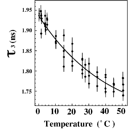
Figure 3: $\tau_{3}$ in water as a function of temperature. Dots show data. Vertical lines show errors. The solid line shows a fitting result by Ps-bubble model combined with the two-state model.

The $\tau_{3}$ decreases smoothly by 10% as the temperature is raised from 0^∘C to 50^∘C. Our $\tau_{3}$ at 20^∘C, $1.839\pm 0.015$ ns, agrees with the measurement of Mogensen, 1.85 ns Mogensen_water .

Behaviors of other lifetime parameters are shown in Fig. 4.

Figure 4: Temperature dependencies of lifetimes, $\tau_{1}$ and $\tau_{2}$ in water and intensities of three lifetime components. Dots show data and vertical lines indicate the fitting error. Solid lines are results of linear regression. a, b: lifetime component $\tau_{1},\tau_{2}$, respectively, c: intensities of three components.

We confirmed that the behavior of $\tau_{3}$ is not caused by a change in other lifetime parameters. To do so, we produced artificial spectra that represent a sum of three exponentials, $\sum_{i=1}^{3}I_{i}\exp(t/\tau_{i})/\tau_{i}$, convoluted by a Gaussian time resolution. The number of events in each 0.0495 ns time bin was made to follow a Poisson distribution. We produced such artificial data samples with different $\tau_{i}$ and $I_{i}$, and fitted for them. Figure 5 shows the fitted $\tau_{3}$ as a function of the varied parameters. Solid lines show the linear fit to the points. First, the fitted $\tau_{3}$ agrees with the input $\tau_{3}$ within $0.01\pm 0.01$ ns, as shown in Fig. 5(c). Second, the fitted $\tau_{3}$ does not depend on $\tau_{1}$, $\tau_{2}$, $I_{2}$, and $I_{3}$. Horizontal bars show the variations and errors of parameters in the measured temperature range. The maximum deviation of $\tau_{3}$ is calculated by multiplying the slope of the linear fit and the quadratic sum of the variation and the error of the other parameters. Deviations resulting from $\tau_{1}$, $\tau_{2}$, $I_{2}$, and $I_{3}$ are $0.000\pm 0.004$ ns, $0.0014\pm 0.0008$ ns, $0.0015\pm 0.0029$ ns, and $0.001\pm 0.003$ ns, respectively. The only apparent dependence is on $I_{1}$, as shown in Fig. 5(d); its effect on $\tau_{3}$ is $0.009\pm 0.002$ ns. The total effect on $\tau_{3}$ that is attributable to the error and swing of other parameters in the temperature range is 0.011 ns. Consequently, we can conclude that the temperature dependence of $\tau_{3}$ is not caused by changes in other lifetime parameters.

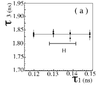
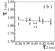
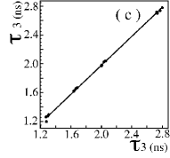
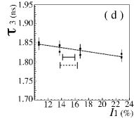
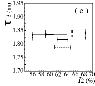
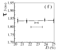
Figure 5: Fitted $\tau_{3}$ as a function of other parameters studied with artificial data samples: (a) $\tau_{1}$, (b) $\tau_{2}$, (c) $\tau_{3}$, (d) $I_{1}$, (e) $I_{2}$, and (f) $I_{3}$. Horizontal solid bars show averages of the standard deviations of parameters at each temperature point; dashed bars show the maximum changes of parameters between 0 and 50^∘C.

V Discussion

The behavior of our $\tau_{3}$ cannot be explained by the original Ps-bubble model. For that reason, we apply the two-state mixture model to the Ps-bubble model. Vedamuthu $et\ al.$ showed that the two-state mixture model can reproduce density of $\mbox{H}_{2}\mbox{O}$ in the temperature range between -30 and +70^∘C with very high precision Vedamuthu94 . In this model, liquid water comprises two dynamically inter-converting mixed micro-domains whose bonding characteristics are similar to those of ice I$h$ (lower density) and ice II (higher density) Urquidi PRL 99 . The total specific volume of liquid water is given as

$$V(T,P)=[1-f_{\mbox{II}}(T,P)]V_{\mbox{I}}(T,P)+f_{\mbox{II}}(T,P)V_{\mbox{II}}(T,P),$$ (5)

where I (II) indicates lower (higher) density bonding, $f_{\mbox{II}}$ is the mass fraction of the higher density bonding type, and $V_{\mbox{I(II)}}$ is the specific volume of the lower (higher) density type bond.

We modified the Ps-bubble model by introducing the two-state mixture model with the following assumptions.

1. Positronium forms a bubble (Ps-bubble) with a radius $R$ in water as the original Ps-bubble model.

2. Water consists of two different molecular bond types, I and II; the ratio $f_{\mbox{II}}$ is a function of the temperature as given by Vedamuthu $et\ al$. Vedamuthu94 .

3. The pick-off rate is determined by an overlap between the $o$-Ps wave function and the electron wave function of the water; it can be parameterized by exuding depths, $\Delta R_{\mbox{I}}$ and $\Delta R_{\mbox{II}}$ for each bonding type.

4. The bubble radius, $R$, is given by a macroscopic surface tension $\gamma$, which is determined by the temperature gamma , $\Delta R_{\mbox{I}}$ and $\Delta R_{\mbox{II}}$ .

The modified equation (1) is:

$$\tau_{3}=\biggl{[}2\biggl{\{}1-\frac{R}{R+(1-f_{\mbox{II}})\Delta R_{\mbox{I}}+f_{\mbox{II}}\Delta R_{\mbox{II}}}+\frac{1}{2\pi}\sin\biggl{(}\frac{2\pi R}{R+(1-f_{\mbox{II}})\Delta R_{\mbox{I}}+f_{\mbox{II}}\Delta R_{\mbox{II}}}\biggr{)}\biggr{\}}\biggr{]}^{-1}.$$ (6)

Figure 3 shows the fitted $\tau_{3}$ using Eq. (6) as a function of temperature. The fitting parameters are $\Delta R_{\mbox{I}}$ and $\Delta R_{\mbox{II}}$. The reduced $\chi^{2}$ is $1.7$. The modified Ps-bubble model represent the temperature dependence of $\tau_{3}$ well.

The fitted exuding depths are $\Delta R_{\mbox{I}}=0.130\pm 0.005$ nm and $\Delta R_{\mbox{II}}=0.218\pm 0.003$ nm. In the Ps-bubble model, $\Delta R$ should correlate with the van der Waals radius of the surrounding atoms. In fact, $\Delta R$, which is determined by fitting data of well-characterized small-pore materials such as zeolites for Eq. (1), is 0.166 nm ujihira ; Nakanishi88 , which agrees with the 0.166 nm average of van der Waals radii of atoms of SiO₄, the main component of zeolite. In our result, $\Delta R_{\mbox{I}}$ = 0.130 nm is close to the van der Waals radius of oxygen (0.155 nm) and hydrogen (0.120 nm). Contrarily, $\Delta R_{\mbox{II}}$ is too large for the van der Waals radius. This indicates that the higher density state has a larger contribution to the pick-off process than their own depth of the electron wave function. This constitutes evidence that the higher density state, which has a bending hydrogen bond Urquidi PRL 99 , is more active than the lower density state.

Next, the fitted $R$ supports the Ps-bubble idea. As shown in Fig. 6, the radius of the Ps-bubble, $R$, based on our fit, is about 0.3 nm.

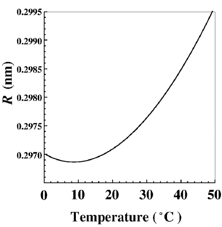
Figure 6: Temperature dependence of the Ps-bubble radius, as calculated with $\gamma$ and fitted $\Delta R_{\mbox{I}}$ and $\Delta R_{\mbox{II}}$.

Liquid water has intrinsic vacancies in its structure while its structure is changing rapidly. Those vacancies produce a hexagonal structure having an oxygen atom at each vertex connected by hydrogen bonds. Considering the distance between the nearest O$\cdots$O, 0.28 nm Bosio83 , and the van der Waals radius of water, the vacancy is smaller than a Ps-bubble. Therefore $o$-Ps should spread water molecules apart to exist in water. This fact supports the need for a balance between the zero-point of $o$-Ps energy and the surface tension of water.

In addition, our model shows that $R$ has a minimum at 8^∘C. The radius of Ps-bubble at 50^∘C is 1.009 times the radius at 8^∘C. This size relationship is consistent with the fact that the distance between the nearest neighbors of O$\cdots$O pair at 50^∘C is 1.011 times the distance at 4^∘C Narten67 .

VI Conclusion

We precisely measured the temperature dependence of the long lifetime of a positron ($\tau_{3}$) in water at temperatures between 0 and 50^∘C. The $\tau_{3}$ decreases smoothly as temperature rises; it is $1.839\pm 0.015$ ns at 20^∘C. This fact is explained by combining two models in which the water consists of two types of molecular bonds, and in which positroniums push those bonds apart to form Ps-bubbles. We also found that $\tau_{3}$ is sensitive to the electron states of the two types of molecular bonds.

References

- (1) W. Brandt, S. Berko, and W.W. Walker, Phys. Rev., 120, 1289 (1960).
- (2) W. Brandt and I. Spirn, Phys. Rev., 142, 231 (1966).
- (3) S. J. Tao, J. Chem. Phys., 56, 5499(1972).
- (4) A. Vértes et al., Journal of Radioanalytical and Nuclear Chemistry, 203, 399 (1996).
- (5) M. Eldrup, D. Lightbody, and J. N. Sherwood, Chem. Phys., 63, 51 (1982).
- (6) O. E. Mogensen, Positron Annihilation in Chemistry, (Springer-Verlag, Berlin, 1995) p.54.
- (7) H. Nakanishi, S. J. Wang, and Y. C. Jean, Positron and Positronium Chemistry, D. M. Schrader and Y. C. Jean (eds.), (Elsevier Sci., Amsterdam, 1988) p.292.
- (8) F. M. Jacobsen, thesis, Risoe-R-433 (1981).
- (9) F. James, CERN Program Library, Entry D 506, Ver. 92.1 (1992).
- (10) P. Kirkegaard, M. Eldrap, O. E. Mogensen, and N. J. Pedersen, Comp. Phys. Comm., 23, 307 (1981).
- (11) F. M. Jacobsen, O. E. Mogensen, and N. J. Pederson, in Positron annihilation, Proceedings of the 8th International Conference, Belgium, edited by L. Dorikens-Vanpraet, M. Dorikens, and D. Segers (1989).
- (12) M. Vedamuthu, S. Singh, and G. W. Robinson, J. Phys. Chem., 98, 2222 (1994).
- (13) J. Urquidi, S. Singh, C. H. Cho, and G. W. Robinson, Phys. Rev. Lett., 83, 2348 (1999).
- (14) N. B. Vargaftic, B. N. Volkov, and J. L. Iborra, J. Phys. Chem. Ref. Data, 98, 817 (1983).
- (15) H. Nakanishi and Y. Ujihira, J. Phys. Chem., 86, 4446 (1982).
- (16) L. Bosio, S.-H. Chen, and J. Teixeira, Phys. Rev. A, 27, 1468 (1983).
- (17) A. H. Narten, M. D. Danford, and H. A. Levy, Discuss. Faraday Soc., 43, 97, (1967).