A Star Based Model for the Eigenvalue Power Law of Internet Graphs

Abstract

Using a simple deterministic model for the Internet graph we show that the eigenvalue power law distribution for its adjacency matrix is a direct consequence of the degree distribution and that the graph must contain many star subgraphs.

1 Introduction

Recent research shows that most communications networks, like the world wide web, the Internet, telephone networks, transportation systems (including the power distribution network), and biological and social networks, belong to a class of networks known as small-world scale-free networks. These networks exhibit both strong local clustering (nodes have many mutual neighbors) and a small diameter (maximum distance between any two nodes) [13]. Another important common characteristic is that the number of links attached to the nodes usually obeys a power law distribution (is scale-free) as was observed first in empirical studies from the Faloutsos’ brothers [10] and Barábasi and Albert [1]. In [10], the authors present data that show that the eigenvalue distribution of the adjacency matrix of the Internet graph also follows a power law. A qualitative proof that this power-law is a consequence from the distribution of degrees of the network, which should contain many star subgraphs of different sizes, was presented by the authors in [3]. Mihail and Papadimitriou in [11] provided an analytical proof by using the theory of random graphs. Fabrikant, Koutsoupias and Papadimitriou [9] provide an explanation of the Internet power laws based on complex multicriterion optimization.

Many approaches to understanding small-world scale-free networks are based on stochastic models and computer simulations, however the use of deterministic models (although they do not allow to capture the full complexity of a real life network) do help in the understanding of their behavior and permit the direct determination of relevant parameters for the modeled networks. In particular, it is possible to construct small-world deterministic graphs with different degree distributions matching the distribution of real networks, see [5, 2, 7, 4]. We introduce in this paper a simple deterministic model, a toy model, to show analytically, that the observed eigenvalue power law of the Internet may be a direct consequence of the degree distribution of a star based structure (whose power law can be justified considering, for example, preferential attachment [1] or duplication [6] models).

2 A star graphs based deterministic model

Restricting our study to the Internet graph (at the router level), our model considers this graph as a scale-free network made by the union of a number of star graphs with different orders and connected through the root vertices by a relatively small backbone graph $B$, see Figure 1.

Figure 1: (a) A simple model for the Internet graph: many degree one nodes are attached to a backbone graph $B$ to form graph $G$. (b) Deleting the backbone graph $B$ results in a non connected graph constituted by the union of star graphs.

This model is an approximation to the real Internet graph, as described in appendix A of [10], if we consider a degree distribution matching the observed results:

Each $n_{i}+1$-star graph (with a root node and $n_{i}$ other nodes) will contribute with a vertex of degree $n_{i}$ and $n_{i}$ vertices of degree $1$. The eigenvalues of this star graph are $\pm\sqrt{n_{i}}$ and $0$.

If we consider a set of star graphs whose root vertices have rank degrees distributed according to a power law $\beta$, the graph union of these graphs will have eigenvalues with ranks distributed according to $\frac{\beta}{2}$. We note that, as we are considering a determinitic exact model, to relate the exponent of the discrete degree distribution to the $\beta$ exponent of a continuous degree distribution for a random scale-free graph, a cumulative distribution should be considered, $P_{cum}(k)\equiv\sum_{k^{\prime}\geq k}n(k^{\prime})/N\sim k^{1-\beta}$, where $k$ and $k^{\prime}$ are values of the discrete degree spectrum, $n(k^{\prime})$ is the number of vertices of degree $k^{\prime}$ and $N$ is the order of the graph.

It is possible now to give some insight on the eigenvalues of the global graph $G$ obtained by joining the star graphs by using a backbone graph $B$. Since the number of vertices of $B$ is small with respect to the total number of vertices of all the star graphs, the values of the spectrum will be very close to the original graph of stars and will therefore follow a power law.

This last result is related to the interlacing theorem [8] which states that if $\Gamma$ is a graph with spectrum $\lambda_{1}\geq\lambda_{2}\geq\dots\geq\lambda_{p}$, $v_{1}$ is a vertex of $\Gamma$, and $\mu_{1}\geq\mu_{2}\geq\dots\geq\mu_{p-1}$ is the spectrum of $\Gamma\setminus v_{1}$ (the graph resulting from $\Gamma$ after deleting $v_{1}$ and its associated edges) then the spectrum of $\Gamma\setminus v_{1}$ is interlaced with the spectrum of $\Gamma$, i.e. $\lambda_{1}\geq\mu_{1}\geq\lambda_{2}\geq\mu_{2}\geq\dots\geq\mu_{p-1}\geq\lambda_{p}$.

On the other hand, notice that this simple model ensures that if the power-law exponent for the degrees is $\beta$, the corresponding exponent for graph $G$ will be approximately $\beta/{2}$, matching the results shown in  [10].

In the next section we compute analitically the eigenvalues of $G$ and verify that they are close to those of its star subgraphs.

3 Analytical computation of the eigenvalues of $G$

Consider $s$ star graphs $S_{1},S_{2},\dots,S_{s}$ with, respectively, $n_{1}+1,n_{2}+1,\dots,n_{s}+1$ vertices. The backbone graph $B$ joins the central vertices of each star. We call $A$ the adjacency matrix of this graph $B$. This is equivalent to start with a graph $B$ with $s$ vertices and add to each vertex, respectively, $n_{1},\dots,n_{s}$ new vertices of degree 1.

To compute the spectrum of the global graph $G$ ($B$ plus the vertices of degree one) we consider $\left(\begin{array}[]{cc}A&b^{T}\\ b&O\end{array}\right)\left(\begin{array}[]{c}x\\ y\end{array}\right)=\lambda\left(\begin{array}[]{c}x\\ y\end{array}\right)$ which gives the system to solve

$$\Bigg{\{}\begin{array}[]{l}Ax+b^{T}y=\lambda x\\ bx=\lambda y\end{array}$$ (1)

where $b^{T}=\mbox{\rm diag}(b_{1},\dots,b_{s})$ with $b_{i}=(1,\dots,1)$, $n_{i}$ ones, i.e. $b^{T}$ is a $s\times(\sum_{i=1}^{s}n_{i})$ matrix and $O$ is the null matrix with dimensions $(\sum_{i=1}^{s}n_{i})\times(\sum_{i=1}^{s}n_{i})$.

If $\lambda\neq 0$, from (1) we obtain $Ax+\lambda^{-1}b^{T}bx=\lambda x$ where $b^{T}b$ is a diagonal matrix, whose elements are $n_{1},\dots,n_{s}$. Thence $Ax=(\lambda I-\lambda^{-1}\mbox{\rm diag}(n_{1},\dots,n_{s}))x$. Introducing $\alpha_{i}=\lambda/(\lambda^{2}-n_{i})$, this last equation can be written

$$\mbox{\rm diag}(\alpha_{1},\dots,\alpha_{s})Ax=x.$$ (2)

If the backbone graph $B$ is another star graph with $s$ nodes (rooted in one of the star graphs), then the matrix $A$ will be $\left(\begin{array}[]{cc}0&b^{T}\\ b&O_{s-1}\end{array}\right)$ where $b^{T}=(1,\dots,1)$ and $O_{s-1}$ is a null matrix of dimensions $(s-1)\times(s-1)$. Thus, the eigenvalues of $G$ are the values of $\lambda$ wich verify (2) for this $A$, i.e. values which allow the matrix $\mbox{\rm diag}(\alpha_{1},\dots,\alpha_{s})A$ to have 1 as eigenvalue.

Solving $\det(\mbox{\rm diag}(\alpha_{1},\dots,\alpha_{s})A-xI)=0$ we find

$$(-x)^{s-2}\left(x^{2}-\alpha_{1}\sum_{i=2}^{s}\alpha_{i}\right)=0$$ (3)

and the eigenvalues are $0$ with multiplicity $s-2$, and $\pm\sqrt{\alpha_{1}\sum_{i=2}^{s}\alpha_{i}}$ with multiplicity $1$. Hence, the final equation to solve is $\alpha_{1}\sum_{i=2}^{s}\alpha_{i}=1.$ Its left part is a function of $\lambda$

$$\begin{array}[]{lll}f(\lambda)&=&\alpha_{1}\sum_{i=2}^{s}\alpha_{i}=\sum_{i=2}^{s}\alpha_{1}\alpha_{i}=\sum_{i=2}^{s}\frac{\lambda}{\lambda^{2}-n_{1}}\frac{\lambda}{\lambda^{2}-n_{i}}\\ &=&\sum_{i=2}^{s}\frac{n_{1}}{(n_{1}-n_{i})(\lambda^{2}-n_{1})}-\frac{n_{i}}{(n_{1}-n_{i})(\lambda^{2}-n_{i})}\end{array}$$

and it can be decomposed in a sum of simple fractions whose asymptotes are given by $\lambda_{i,\pm}=\pm\sqrt{n_{i}}$. The points $\lambda^{\prime}_{i}$ where this rational function cuts the constant function $1$ are the solutions of the equation, and they are therefore the eigenvalues of $G$ we are looking for, see Figure 2.

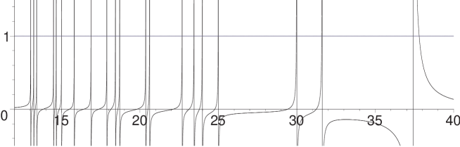
Figure 2: Analytical determination of the eigenvalues of graph $G$, the graph obtained by joining several star graphs with a backbone graph.

Each fraction $\frac{1}{\lambda^{2}-n_{i}}$ can be decomposed as $\frac{1}{2\sqrt{n_{i}}(\lambda-\sqrt{n_{i}})}-\frac{1}{2\sqrt{n_{i}}(\lambda+\sqrt{n_{i}})}$. If we consider the positive values to find the largest eigenvalues and assuming $n_{1}\geq\dots\geq n_{s}$, for $2\leq i\leq s$ approaching the value $\sqrt{n_{i}}$ from the right, the function $f(\lambda)$ is negative, whereas approaching it from the left it is positive. Therefore it should cut the constant function $1$ in the left side, so $\lambda^{\prime}_{i}<\sqrt{n_{i}}$, and $\lambda^{\prime}_{i}>\sqrt{n_{i+1}}$ as at $\sqrt{n_{i+1}}$ there is another asymptote and the function is negative on the right side of $\sqrt{n_{i+1}}$. Therefore the eigenvalues of $G$ verify: $\sqrt{n_{i}}>\lambda^{\prime}_{i}>\sqrt{n_{i+1}}$ and $\lambda^{\prime}_{i}=\sqrt{n_{i}}-\Delta$, where $\Delta<\sqrt{n_{i}}-\sqrt{n_{i+1}}$. At $\sqrt{n_{1}}$ the function is positive at the right of this point and negative at the left. Hence, $\lambda^{\prime}_{1}\geq\sqrt{n_{1}}$.

Note that if the values for $n_{i}$ are consecutive integers, the difference in the corresponding square roots will be very small for large $n_{i}$ and the eigenvalues for the new graph will be very near to those of the disconnected star graphs.

Example 1

Consider the Oregon-Multi dataset of Internet at the AS level as in 2001 [12], and use a star graph as backbone graph $B$ to interconnect the star graphs with $n_{i}$ equal to 1400, 1000, 900, 625, 575, 550, 515, 425, 415, 350, 340, 320, 285, 250, 225, 215, 210, 180, 175 and 170. The degree distribution (by construction) fits the degree distribution of the Internet graph as shown in [12]. To calculate the spectra of this graph we solve the equation $f(\lambda)=1$ and we obtain: 13.03, 13.22, 13.41, 14.48, 14.66, 14.99, 15.81, 16.87, 17.88, 18.43, 18.70, 20.36, 20.61, 22.68, 23.44, 23.96, 24.98, 29.97, 31.59, 37.80.

In Figure 3 we plot the twenty highest eigenvalues in a log-log scale. The result shows a power law as in the real data from  [12]. Observe that the slope of the regression model is very similar to the observational data.

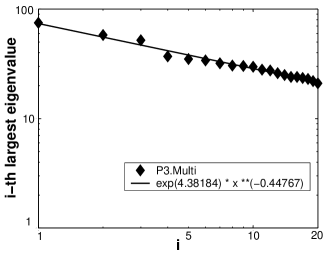
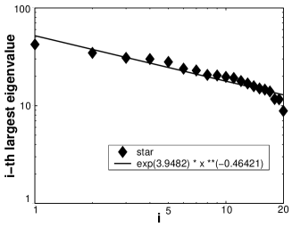
Figure 3: Highest twenty eigenvalues for the Internet graph (Oregon-Multi), see [12], and the graph constructed in Example 1. In both cases they follow a power law.

4 Other models and conclusions

The model considered here describes the degree and eigenvalue distributions of the Internet graph, however its clustering is zero as the resulting graph is a tree. We have performed the same analysis connecting the root vertices of the star graphs with a complete graph. The results are comparable to those obtained above (in that case the clustering of the global graph is different from zero but small). We note that if the backbone graph $B$ joins complete graphs instead of star graphs this would lead to an eigenvalue power law with an exponent close to the exponent of the degree distribution (the eigenvalues of a complete graph with $n$ vertices are $n-1$ and $-1$).

The star-based model considered here constitutes a convenient tool to study the Internet network since using deterministic techniques no simulation is needed and relevant network parameters can be directly calculated. Thus, the contrast of real with synthesized networks is straightforward. On the other hand, our study shows that it is a reasonable assumption to consider that the Internet graph contains many star subgraphs, as this explains the observed power-laws and relationship between the degree and eigenvalue distributions.

Acknowledgment

This research was supported by the Secretaria de Estado de Universidades e Investigación (Ministerio de Educación y Ciencia), Spain, and the European Regional Development Fund (ERDF) under project TIC2002-00155.

References

- [1] A.-L. Barabási, R. Albert, Emergence of scaling in random networks, Science 286 (1999) 509–512.
- [2] A.-L. Barabási, E. Ravasz, T. Vicsek, Deterministic scale-free networks, Physica A 299 (2001) 559-564.
- [3] F. Comellas, Deterministic small-world graphs, Contributed Talk at the Int. Conf. on Dynamical Networks in Complex Systems, July 25-27, Kiel, Germany, (Europhysics Conference Abstracts, vol 25F , 2001, pag. 18).
- [4] F. Comellas, G. Fertin, A. Raspaud, Recursive graphs with small-world scale-free properties, Phys. Rev. E 69 (2004) 037104.
- [5] F. Comellas, J. Ozón, J.G. Peters, Deterministic small-world communication networks, Inform. Process. Lett. 76 (2000) 83–90.
- [6] F. Chung, Linyuan Lu, T. G. Dewey, D. J. Galas, Duplication models for biological networks, J. of Comput. Biology 10 (5) (2003) 677–688.
- [7] F. Comellas, M. Sampels, Deterministic small-world networks, Physica A 309 (1-2) (2002) 231–235.
- [8] D. M. Cvetkovic, M. Doob, H. Sachs, Spectra of Graphs, Theory and Applications, 3rd ed., Johann Ambrosius Barth, Heidelberg, 1995.
- [9] A. Fabrikant, E. Koutsoupias, C. Papadimitriou, Heuristically optimized trade-offs: A new paradigm for power laws in the Internet, Proc. ICALP 2002. LNCS 2380 (2002) 110–122.
- [10] M. Faloutsos, P. Faloutsos, C. Faloutsos, On power-law relationships of the Internet topology, In Proceedings of the ACM SIGCOMM, pages 251–262, August 1999.
- [11] M. Mihail, C. Papadimitriou, On the eigenvalue power law, LNCS 2483 (2002) 254–262.
- [12] G. Siganos, M. Faloutsos, P. Faloutsos, C. Faloutsos, Power laws and the AS-level Internet topology, IEEE/ACM Trans. Networking 11 (4) (2003) 514–524.
- [13] D.J. Watts, S.H. Strogatz, Collective dynamics of ‘small-world’ networks, Nature 393 (1998) 440–442.