Effective temperature in the quench of coarsening systems to and below $T_{C}$

Abstract

We overview the general scaling behavior of the effective temperature in the quenches of simple non disordered systems, like ferromagnets, to and below $T_{C}$. Emphasis is on the behavior as dimensionality is varied. Consequences on the shape of the asymptotic parametric representation are derived. In particular, this is always trivial in the critical quenches with $T_{C}>0$. We clarify that the quench to $T_{C}=0$ at the lower critical dimensionality $d_{L}$, cannot be regarded as a critical quench. Implications for the behavior of the exponent $a$ of the aging response function in the quenches below $T_{C}$ are developed.

‡corberi@sa.infn.it †lippiello@sa.infn.it §zannetti@na.infn.it

keywords

Coarsening processes (Theory), Slow dynamics and aging (Theory)

I Introduction

In the study of slow relaxation phenomena [1], typically, a temperature quench is made at time $t=0$ and the quantities of interest, such as the autocorrelation $C(t,t_{w})$ and the linear response function $R(t,t_{w})$, are monitored at subsequent times $0<t_{w}<t$. The peculiar and interesting feature of these processes is that equilibrium is never reached, namely there does not exist a finite time scale $t_{eq}$ such that for $t_{w}>t_{eq}$ two time quantites become time translation invariant.

A substantial progress in the study of these phenomena has been achieved after Cugliandolo and Kurchan [2] have introduced the modification of the fluctuation-dissipation theorem (FDT) as a quantitative indicator of the deviation from equilibrium [3]. This can be formulated in several equivalent ways. Here, we find convenient to use the effective temperature [4]

$$T_{eff}(t,t_{w})={\partial_{t_{w}}C(t,t_{w})\over R(t,t_{w})}$$ (1)

which coincides with the temperature $T$ of the thermal bath if the FDT holds, that is in equilibrium, while it is different from $T$ off equilibrium. Because of the absence of a finite equilibration time, the characterization of the system staying out of equilibrium for an arbitrarily long time is contained in $\lim_{t_{w}\to\infty}T_{eff}(t,t_{w})$. However, since $t_{w}\rightarrow\infty$ implies also $t\rightarrow\infty$, to make the limit operation meaningful one must specify how the two times are pushed to infinity. One way of doing this is to fix the value of the autocorrelation function $C(t,t_{w})$ as $t_{w}\rightarrow\infty$. More precisely, since $C(t,t_{w})$ for a given $t_{w}$ is a monotonously decreasing function of $t$, the time $t$ can be reparametrized in terms of $C$ obtaining $T_{eff}(t,t_{w})=\widehat{T}_{eff}(C,t_{w})$ and, keeping $C$ fixed, the limit

$${\cal T}(C)=\lim_{t_{w}\to\infty}\widehat{T}_{eff}(C,t_{w})$$ (2)

defines the effective temperature in the time sector corresponding to the chosen value of $C$. This quantity is important because, when appropriate conditions are satisfied, provides the connection between dynamic and static properties [7] through the relation

$$P(q)=T{d\over dC}{\cal T}(C)^{-1}|_{C=q}$$ (3)

where $P(q)$ is the overlap probability function of the equilibrium state. Therefore, different shapes of ${\cal T}(C)$ are associated to different degrees of complexity of the equilibrium state. A first broad classification of systems has been made [8, 9] drawing the distinction between coarsening systems, structural glasses and the infinite range spin glass model on the basis of the patterns displayed by ${\cal T}(C)$, or related quantities such as the fluctuation-dissipation ratio (FDR) and the zero field cooled (ZFC) susceptibility. In this paper we focus on coarsening systems, exemplified by a non disordered and non frustrated system such as a ferromagnet, relaxing via domain growth after a quench to or below the critical point [10, 11, 12]. We show that even within the framework of these so called trivial systems, the spectrum of the behaviors of ${\cal T}(C)$ is quite rich and interesting.

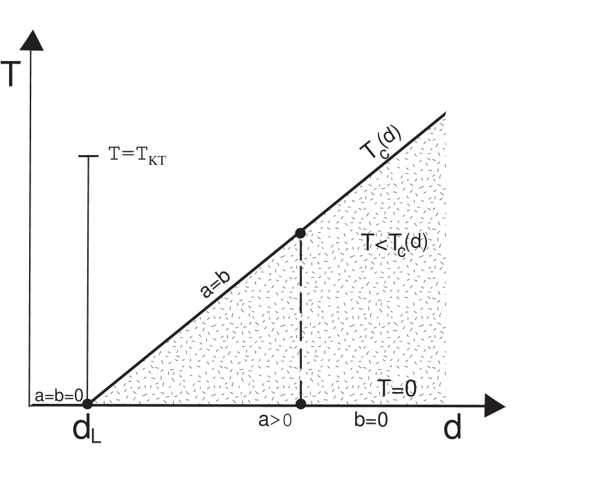
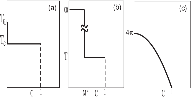
In order to illustrate the problem, in Fig.1 we have drawn schematically the phase diagram, in the temperature-dimensionality plane. The critical temperature vanishes at the lower critical dimensionality $d_{L}$. The disordered and ordered phase are, respectively, above and below the critical line $T_{C}(d)$. Slow relaxation arises for quenches with the final temperature everywhere in the shaded area, including the boundary. Usually, one considers some fixed $d>d_{L}$ (dashed line in Fig.1) and studies the quench to a final temperature $T\leq T_{C}$. The form of ${\cal T}(C)$ in the critical quench with $T=T_{C}$ (Fig.2a) is different from that with $T<T_{C}$ (Fig.2b) and both are independent of $d$. The interesting question, then, is what happens at the special point $(d_{L},T=0)$, where critical and subcritical quenches merge. Namely, will ${\cal T}(C)$ display continuity with the critical or with the subcritical shape? On the basis of the available evidence from analytical solutions [13, 14, 15, 16] and numerical simulations [17] , the surprising answer is with neither of them. A third and nontrivial form of ${\cal T}(C)$ is found (Fig.2c) in the quench to $(d_{L},T=0)$.

In this paper we present the scaling framework which allows to account in a unified way for this wealth of behaviors displayed by ${\cal T}(C)$ upon letting $T$ and $d$ to vary. This, in turn, allows to gain insight on the challanging problem [16, 18] of the scaling of $R(t,t_{w})$ in the quenches below $T_{C}$. Furthermore, on the basis of these ideas, predictions can be made for the interesting case of the XY model. In that case, the phase diagram of Fig.1 is enriched by the presence of the Kosterlitz-Thouless (KT) line of critical points at the lower critical dimensionality $(d_{L}=2)$, with $T\leq T_{KT}$. Therefore, slow relaxation in the XY model arises also by arranging the quenches onto the KT line. Since this is a critical line, the phenomenology for $0<T\leq T_{KT}$ is expected to be akin to the one along the $T_{C}(d)$ line, while at $T=0$ the switch to the third nontrivial form of ${\cal T}(C)$ is expected to take place.

The paper is organised as follows. In section II the scaling properties of $C(t,t_{w})$ and $R(t,t_{w})$ are reviewed. In section III the general scaling behavior of $T_{eff}(t,t_{w})$ is derived, and in section IV the parametric form ${\cal T}(C)$ is obtained. The problem of the exponent $a$ of $R(t,t_{w})$ below $T_{C}$ is presented in section V. Sections VI and VII are devoted to the illustration of the general concepts in the context of the large-$N$ model and of the $XY$ model, respectively. Conclusions are presented in section VIII.

II Scalings of $C(t,t_{w})$ and $R(t,t_{w})$

In the following we consider quenches from an initial disordered state above the critical line to any one of the states in the shaded area of Fig.1. For definiteness, we shall refer to purely relaxational dynamics without conservation of the order parameter, but the results are of general validity. The common feature of all these processes is that, after a short transient, dynamical scaling sets in with a characteristic length growing with the power law $L(t)\sim t^{1/z}$ [10]. The scaling properties with $T=T_{C}$ are different from those with $T<T_{C}$ [11]. In the renormalization group language this means that for a given $d$ there are two fixed points, one unstable at $T_{C}$ and the other stable and attractive at $T=0$ (thermal fluctuations are irrelevant below $T_{C}$) [19]. The dynamical exponent $z$ on the $T_{C}(d)$ line coincides with the dynamical critical exponent $z_{c}$ and depends on dimensionality, while below criticality it takes the dimensionality independent value $z=2$. These values become identical at $(d_{L},T=0)$, since $\lim_{d\to d_{L}}z_{c}=2$ [20].

Let us, next, review the scaling properties of $C(t,t_{w})$ and $R(t,t_{w})$. The fixed point structure enters in two ways: in the values of the exponents involved and, less obviously, in the very same form of the functions $C(t,t_{w})$ and $R(t,t_{w})$. In analysing the asymptotic behavior of these quantities, it is necessary to distinguish between the short time and the large time behaviors obtained by letting the waiting time $t_{w}$ to become large, while keeping, respectively, either the time difference $\tau=t-t_{w}$ or the time ratio $x=t/t_{w}>1$ fixed. Notice that from $x=1-\tau/t_{w}$ follows that the short time regime, when using the $x$ variable, gets compressed into $x=1$.

An important general property of two time quantities in slow relaxation phenomena is that in the short time regime the system appears equilibrated and the FDT is satisfied, while the off equilibrium character of the dynamics, or aging, shows up in the large time regime [1, 3, 12]. The mechanism underlying this property, however, is quite different for quenches to and below $T_{C}$.

A Critical quench: multiplicative structure

In the critical quenches, for $t_{w}$ sufficiently large, $C(t,t_{w},t_{0})$ and $R(t,t_{w},t_{0})$ take the product forms [11, 12]

$$C(t,t_{w},t_{0})=(\tau+t_{0})^{-b}g_{C}(x,y)$$ (4)

$$R(t,t_{w},t_{0})=(\tau+t_{0})^{-(1+a)}g_{R}(x,y)$$ (5)

where $g_{C,R}(x,y)$ are smooth functions of $x$ with a weak dependence on $y=t_{0}/t_{w}$. In addition to the observation times, $t$ and $t_{w}$, we have explicitely included also the dependence on a microscopic time $t_{0}$, which is needed to regularize these functions at equal times. In particular, we shall take $C(t,t,t_{0})=1$ throughout. In the short time regime

$$C(t,t_{w},t_{0})=(\tau+t_{0})^{-b}g_{C}(1,0)$$ (6)

$$R(t,t_{w},t_{0})=(\tau+t_{0})^{-(1+a)}g_{R}(1,0)$$ (7)

which are the autocorrelation and response function of the stationary critical dynamics satisfying, therefore, the equilibrium FDT, i.e. $T_{C}R(\tau)=-\partial_{\tau}C(\tau)$, which implies

$$T_{C}g_{R}(1,0)=bg_{C}(1,0)$$ (8)

and

$$a=b.$$ (9)

We emphasize that, in the critical quench, as a consequence of the multiplicative structure and of the FDT, the exponents $a$ and $b$ are not independent and coincide. Furthermore, their common value is given by [11, 12]

$$a=b=(d-2+\eta)/z_{c}=2\beta/\nu z_{c}$$ (10)

where $\eta$, $\beta$ and $\nu$ are the usual static exponents. Using the geometrical interpretation of the critical properties Eq. (10) can be rewritten as $a=b=2(d-D)/z_{c}$, where $D$ is the fractal dimensionality of the correlated critical clusters [21]. These become compact as $T_{C}\rightarrow 0$ yielding

$$\lim_{d\to d_{L}}a=b=0.$$ (11)

On the KT line, where $d=2$, Eq. (10) is replaced by $a=b=\eta(T)/z$ with $\eta(T)$ vanishing as $T\rightarrow 0$ [22]. Eqs. (4) and (5) can be recast in the simple aging form

$$C(t,t_{w},t_{0})=t_{w}^{-b}f_{C}(x,y)$$ (12)

$$R(t,t_{w},t_{0})=t_{w}^{-(1+a)}f_{R}(x,y)$$ (13)

where

$$f_{C}(x,y)=(x-1+y)^{-b}g_{C}(x,y)$$ (14)

$$f_{R}(x,y)=(x-1+y)^{-(1+a)}g_{R}(x,y).$$ (15)

These functions, for large $x$ and $t_{w}$, decay with the same power law

$$f_{C,R}(x,0)=A_{C,R}x^{-\lambda_{c}/z_{c}}$$ (16)

where $\lambda_{c}$ is the autocorrelation exponent [11, 12].

B Quench below the critical line: additive structure

Below $T_{C}$, the picture is different because the stationary and aging components enter additively into the autocorrelation function [23, 1, 3]

$$C(t,t_{w},t_{0})=C_{st}(\tau)+C_{ag}(t,t_{w},t_{0})$$ (17)

where $C_{st}(\tau)$ is the equilibrium autocorrelation function in the broken symmetry pure state at the temperature $T$. From the equal time properties

$$C(t,t,t_{0})=1\qquad C_{st}(\tau=0)=1-M^{2}$$ (18)

which imply

$$C_{ag}(t,t,t_{0})=M^{2}$$ (19)

where $M$ is the spontaneous magnetization, follows that in Eq. (17) the stationary component corresponds to the quasi-equilibrium decay to the plateau at the Edwards-Anderson order parameter $q_{EA}=M^{2}$, while the aging component $C_{ag}$ describes the off-equilibrium decay from the plateau at much larger times. In the short time regime, then, we have

$$C(\tau+t_{w},t_{w},t_{0})=C_{st}(\tau)+M^{2}$$ (20)

while, taking into account that $C_{st}(\tau)$ vanishes as $\tau\rightarrow\infty$, in the large time regime

$$C(t,t_{w},t_{0})=C_{ag}(t,t_{w},t_{0}).$$ (21)

From this it is easy to verify that, contrary to what happens with the multiplicative structure of Eq. (4), the limits $t_{w}\rightarrow\infty$ and $t\rightarrow\infty$ do not commute

$$\lim_{t\to\infty}\lim_{t_{w}\to\infty}C(t,t_{w},t_{0})=M^{2}$$ (22)

$$\lim_{t_{w}\to\infty}\lim_{t\to\infty}C(t,t_{w},t_{0})=0$$ (23)

yielding the weak ergodicity breaking [1], characteristic of the quenches below $T_{C}$.

The additive structure of the response function

$$R(t,t_{w},t_{0})=R_{st}(\tau)+R_{ag}(t,t_{w},t_{0})$$ (24)

is obtained in the following way [3]: in the short time regime stationarity holds $R(t,t_{w},t_{0})=R_{st}(\tau)$ and $R_{st}(\tau)$ is defined from the FDT

$$R_{st}(\tau)=-{1\over T}{\partial\over\partial\tau}C_{st}(\tau)$$ (25)

whilst $R_{ag}(t,t_{w},t_{0})$ remains defined by Eq. (24). This implies that $R_{ag}(t,t_{w},t_{0})$ vanishes in the short time regime and since, conversely, $R_{st}(\tau)$ vanishes in the large time regime, we may write

$$R(t,t_{w},t_{0})=\left\{\begin{array}[]{ll}R_{st}(\tau)\qquad$for$\qquad x=1\\ R_{ag}(t,t_{w},t_{0})\qquad$for$\qquad x>1.\end{array}\right.$$ (28)

The components $C_{ag}(t,t_{w},t_{0})$ and $R_{ag}(t,t_{w},t_{0})$ obey simple aging forms like (12) and (13) with scaling functions $f_{C,R}(x,y)$ decaying, for large $x$, with a power law of the form (16). It is understood that all the exponents must be replaced by their values below $T_{C}$, which are different from those at $T_{C}$. In particular, from phase ordering theory it is well known [10] that $b=0$ independently from dimensionality. This can be readily understood from $b=2(d-D)/z$, which holds in general, and from the compact nature of the coarsening domains, which gives $D=d$. Quite different is the case of the exponent $a$. Since the FDT relates only the stationary components $C_{st}(\tau)$ and $R_{st}(\tau)$, due to the additive structure of Eqs. (17) and (24) we have no more the constraint $a=b$, as in the critical quench. Namely, in the quench below $T_{C}$ the value of $a$ is decoupled from that of $b$. As a matter of fact, the determination of $a$ below $T_{C}$ is a difficult and challanging problem [17, 18], which will be discussed in section V.

C Quench at $(d_{L},T=0)$: additive structure

As we have seen above, the structures of $C(t,t_{w},t_{0})$ and $R(t,t_{w},t_{0})$ follow different patterns in the quenches to and below $T_{C}$. This raises the question of which one applies when the quench is made at $(d_{L},T=0)$. In other words, should we consider the state $(d_{L},T=0)$ as a critical point with $T_{C}=0$, as it is often done in the literature, or should we consider it as the continuation to $d_{L}$ of the $T=0$ states below criticality? The correct answer is the second one, since at $d_{L}$ the system orders, as in all the states below the critical line, while on the $T_{C}(d)$ line there is no ordering. In particular, this implies that weak ergodicity breaking takes place also in the quench to $(d_{L},T=0)$. From Eqs. (17) and (18) then follows $C_{st}(\tau)\equiv 0$ and

$$C(t,t_{w},t_{0})=f_{C}(x,y)$$ (29)

with $f_{C}(1,0)=1$, since $M^{2}=1$ at $T=0$.

The fact that the quench to $(d_{L},T=0)$ belongs to the additive scheme becomes important when considering the response function, because if $C_{st}(\tau)$ vanishes in the ground state, the same is not true for $R_{st}(\tau)$. Therefore, Eq. (24) holds with $R_{st}(\tau)\neq 0$ and it is important to subtract this contribution from $R(t,t_{w},t_{0})$ if one wants to study the scaling properties of $R_{ag}(t,t_{w},t_{0})$. We shall come back on this point in section VI, when treating the explicit example of the large-$N$ model. It should be mentioned, here, that the linear response function at $T=0$ is well defined only for systems with soft spins. In the case of hard spins there does not exist a linear response regime when $T=0$. For a discussion of this problem and how to bypass it in Ising systems, we refer to [13, 16].

D Comparison with theory

A natural question is how the picture outlined above compares with theoretical approaches. In the case of the quench to $T_{C}$ renormalization group methods are available [24, 12], which account for the multiplicative structure of the autocorrelation and response function and give explicit expressions for the quantities of interst up to two loops order. The development of systematic expansion methods for the quench below $T_{C}$ is much more difficult [25]. Recently, Henkel and collaborators [26, 27] have developed a method based on the requirement of local scale invariance. According to this approach the response function obeys the multiplicative structure (5) both in the quenches to $T_{C}$ and below $T_{C}$. Problems, then, arise in the latter case. The main one is of conceptual nature, since, as explained above, the weak ergodicity breaking scenario requires the autocorrelation function to obey the additive structure (17). Then, in the short time regime, where Eq. (20) holds, from the FDT one has $\partial_{t_{w}}C_{st}(\tau)\sim(\tau+t_{0})^{-(1+a)}$, which implies $C_{st}(\tau)\sim(\tau+t_{0})^{-a}$. In other words, if the local scale invariance prediction for the response function is valid then the stationary correlation function must decay with a power law. This is the case, as we have seen above, in the critical quenches and, as we shall see in section VI, in the large $N$ model. Conversely, in all other cases where the equilibrium correlation function below $T_{C}$ decays exponentially, the response function cannot be of the form (5). Nonetheless, Henkel et al. do criticize [27] the additive structure below $T_{C}$.

The second problem is that existing results, exact [13, 14, 15] and approximated [16, 28, 25] as well as numerical [18, 29], lead to an the aging part of the response function which, for systems with scalar order parameter [30], is of the form

$$R_{ag}(t,t_{w},t_{0})=t_{w}^{-1/z}(\tau+t_{0})^{-(a-1/z+1)}g_{R}(x,y).$$ (30)

This is qualitatively different from the multiplicative form (5), both in the structure and in the exponents. As mentioned above, an exception is the large $N$ model, where $R(t,t_{w},t_{0})$ is of the form (5) also below $T_{C}$. Yet, as we show in section VI, the additive structure applies to the large $N$ model as in all cases of quench below $T_{C}$.

III Effective temperature

The next step is to see how these different behaviors of $C(t,t_{w},t_{0})$ and $R(t,t_{w},t_{0})$ do affect the behavior of $T_{eff}(t,t_{w},t_{0})$.

A Critical quench

From Eqs. (12), (13) and (9), using the definition (1), we get

$$T_{eff}(t,t_{w},t_{0})=F(x,y)$$ (31)

with

$$F(x,y)=-f_{\partial C}(x,y)/f_{R}(x,y)$$ (32)

and

$$f_{\partial C}(x,y)=bf_{C}(x,y)+\left[x{\partial\over\partial x}f_{C}(x,y)+y{\partial\over\partial y}f_{C}(x,y)\right].$$ (33)

In the short time regime, Eqs. (6), (7) and (8) lead to the boundary condition

$$F(1,y)=T_{C}$$ (34)

while, in the aging regime, from Eq. (16) follows

$$\lim_{x\to\infty}F(x,0)=T_{\infty}=\left({\lambda_{c}\over z_{c}}-b\right){A_{C}\over A_{R}}={T_{C}\over X_{\infty}}$$ (35)

where $X_{\infty}$ is the limit FDR of Godrèche and Luck [11].

B Quench below the critical line

Below $T_{C}$, where $b=0$, from the definition (1), the additive structure and Eq. (25) we get

$$T_{eff}(t,t_{w},t_{0}))={TR_{st}(\tau)\over R_{st}(\tau)+R_{ag}(t,t_{w},t_{0})}+{\partial_{t_{w}}C_{ag}(t,t_{w},t_{0})\over R_{st}(\tau)+R_{ag}(t,t_{w},t_{0})}$$ (36)

which can be rewritten as

$$T_{eff}(t,t_{w},t_{0})) = T\left[{R_{st}(\tau)\over R_{st}(\tau)+R_{ag}(t,t_{w},t_{0})}\right]$$ (37)

$$+ t_{w}^{a}F(x,y)\left[{R_{ag}(t,t_{w},t_{0})\over R_{st}(\tau)+R_{ag}(t,t_{w},t_{0})}\right]$$ (38)

where $F(x,y)$ is still defined by Eqs. (32), (33) with $f_{C}(x,y)$, $f_{R}(x,y)$ the scaling functions of $C_{ag}(t,t_{w},t_{0})$ and $R_{ag}(t,t_{w},t_{0})$.

Using Eq. (28) we may approximate Eq. (37) with

$$T_{eff}(t,t_{w},t_{0}))=TH(x)+t_{w}^{a}F(x,y)[1-H(x)]$$ (39)

where

$$H(x)=\left\{\begin{array}[]{ll}1\qquad$for$\qquad x=1\\ 0\qquad$for$\qquad x>1.\end{array}\right.$$ (42)

Therefore, for large $t_{w}$ the general formula containing both critical and subcritical quenches is given by [31]

$$T_{eff}(t,t_{w},t_{0}))=\left\{\begin{array}[]{ll}T\qquad$for$\qquad x=1\\ t_{w}^{a-b}F(x,y)\qquad$for$\qquad x>1.\end{array}\right.$$ (45)

Of course, this includes also the quench to $(d_{L},T=0)$.

IV Parametric representation

In order to derive the parametric representation, as explained in the Introduction, we must express the time dependence of $T_{eff}(t,t_{w},t_{0})$ through $C(t,t_{w},t_{0})$ and then let $t_{w}\rightarrow\infty$, obtaining ${\cal T}(C)$. From Eqs. (4) and (17), for large $t_{w}$, the general form of the autocorrelation function can be written as

$$C(t,t_{w},t_{0})=\left\{\begin{array}[]{ll}1\qquad$for$\qquad x=1\\ t_{w}^{-b}f_{C}(x,y)\qquad$for$\qquad x>1.\end{array}\right.$$ (48)

The task is to eliminate $x$ between Eqs. (45) and (48), which now we do separately for the quenches into the different regions of the phase diagram.

A Critical quench

In this case $a=b>0$. From Eqs. (12) and (14), letting $t_{w}\rightarrow\infty$ with $x$ fixed, we obtain the singular limit

$$C(x)=\left\{\begin{array}[]{ll}1\qquad$for$\qquad x=1\\ 0\qquad$for$\qquad x>1\end{array}\right.$$ (51)

whose inverse is readily obtained exchanging the horizontal with the vertical axis

$$x(C)=\left\{\begin{array}[]{ll}\infty\qquad$for$\qquad C=0\\ 1\qquad$for$\qquad 0<C\leq 1.\end{array}\right.$$ (54)

Inserting into Eq. (45) we obtain (Fig.2a)

$${\cal T}(C)=\left\{\begin{array}[]{ll}T_{\infty}>T_{C}\qquad$for$\qquad C=0\\ T_{C}\qquad$for$\qquad 0<C\leq 1\end{array}\right.$$ (57)

where we have used Eqs. (34) and (35). This is a universal result, since all the non universal features of $F(x,0)$ for the intermediate values of $x$ have been eliminated in the limit process. Therefore, we have that for all quenches to $T_{C}>0$, apart for the value $T_{\infty}$ at $C=0$, the parametric plot of ${\cal T}(C)$ is trivial in the sense that the effective temperature coincides with the temperature $T_{C}$ of the thermal bath. Notice that this implies that for the ZFC susceptibility

$$\chi(t,t_{w})=\int_{t_{w}}^{t}dsR(t,s)$$ (58)

whose parametric form is related to ${\cal T}(C)$ by

$$\chi(C)=\int_{C}^{1}{dC^{\prime}\over{\cal T}(C^{\prime})}$$ (59)

a linear plot is obtained

$$\chi(C)=(1-C)/T_{C}$$ (60)

as for equilibrated systems [3].

B Quench below the critical line

In this case $b=0$ and from Eq. (48) follows

$$C(x)=\left\{\begin{array}[]{ll}1\qquad$for$\qquad x=1\\ f_{C}(x,0)\qquad$for$\qquad x>1\end{array}\right.$$ (63)

where, recalling Eqs. (18) and (21), $f_{C}(x,0)$ is the smooth function describing the fall below the plateau at $M^{2}$. Therefore, the inverse function is given by

$$x(C)=\left\{\begin{array}[]{ll}f_{C}^{-1}(C)>1\qquad$for$\qquad C<M^{2}\\ 1\qquad$for$\qquad M^{2}\leq C\leq 1\end{array}\right.$$ (66)

and inserting into Eq. (45) we find

$$\widehat{T}_{eff}(C,t_{w})=\left\{\begin{array}[]{ll}t_{w}^{a}F(f_{C}^{-1}(C),0)\qquad$for$\qquad C<M^{2}\\ T\qquad$for$\qquad M^{2}\leq C\leq 1.\end{array}\right.$$ (69)

Although the actual value of $a$, as will be explained in section V, is to some extent a debated issue, there is consensus on $a>0$ for $d>d_{L}$. Therefore, taking the $t_{w}\rightarrow\infty$ limit we recover the well known result [1, 3] (Fig.2b)

$${\cal T}(C)=\left\{\begin{array}[]{ll}\infty\qquad$for$\qquad C<M^{2}\\ T\qquad$for$\qquad M^{2}\leq C\leq 1.\end{array}\right.$$ (72)

Again, all the details of $F(x,0)$ having disappeared, the function ${\cal T}(C)$ is universal.

Let us remark, here, as a further manifestation of the difference between quenches to and below $T_{C}$, that the behavior (57) of ${\cal T}(C)$ cannot be recovered by letting $T\rightarrow T_{C}^{-}$ and $M\rightarrow 0$ in (72). In fact, in the latter case we find

$$\lim_{T\to T_{C}^{-}}{\cal T}(C)=\left\{\begin{array}[]{ll}\infty\qquad$for$\qquad C=0\\ T_{C}\qquad$for$\qquad 0<C\leq 1\end{array}\right.$$ (75)

which differs from Eq. (57), where $T_{\infty}$ is a finite number.

C Quench to $(d_{L},T=0)$

If we take the limit $d\rightarrow d_{L}$ in Eqs. (57) and (72) we obtain, respectively

$${\cal T}(C)=\left\{\begin{array}[]{ll}T_{\infty}\qquad$for$\qquad C=0\\ 0\qquad$for$\qquad 0<C\leq 1\end{array}\right.$$ (78)

and

$${\cal T}(C)=\left\{\begin{array}[]{ll}\infty\qquad$for$\qquad C<1\\ 0\qquad$for$\qquad C=1\end{array}\right.$$ (81)

which are very much different one from the other. So, there is the problem of which is the form of ${\cal T}(C)$ in the quench to $(d_{L},T=0)$. A statement to this regard can be made on the basis of the substantial amount of information by now accumulated from sources as diverse as the exact solutions of the $1d$ Ising model [13, 14] and of the $2d$ large-$N$ model [15], the Ohta-Jasnow-Kawasaki type of approximations with $d=1$ [16], in addition to numerical simulations [17] of systems at $d_{L}$ with scalar and vector order parameter, with and without conserved dynamics. In all of these cases we have obtained the parametric plot (59) of the ZFC susceptibility, which gives for ${\cal T}(C)$ at $(d_{L},T=0)$ a non trivial and non universal finite function of the type depicted in Fig.2c. By contrast, there does not exists, up to now, any evidence for behaviors of ${\cal T}(C)$ of the type (78) or (81).

Assuming that the generic behavior of ${\cal T}(C)$ is of the type in Fig.2c, as the amount of evidence quoted above strongly suggests, this is compatible with Eq. (45) only if $a=0$. Then, from Eqs. (63), (66) and (69) with $M^{2}=1$ we may write

$${\cal T}(C)=F(f_{C}^{-1}(C),0)$$ (82)

which represents a smooth, finite, non trivial function deacreasing smoothly from $T_{\infty}=F(\infty,0)$ at $C=0$ toward zero at $C=1$, preserving all the non universal features of $f_{C}(x,0)$ and $F(x,0)$ for the intermediate values of $C$.

D Physical temperature and connection with statics

We conclude this section with comments on the interpretation of ${\cal T}(C)$ as a true temperature and on its connection with the equilibrium properties of the system.

The relation of the effective temperature with a physically measurable temperature is a very interesting issue, which has been thoroughly investigated in Refs. [4, 5, 6]. A necessary condition for the identification of the effective temperature with a true temperature is its uniqueness, that is the indepence from the observable used in the study of the deviation from FDT. For what concerns the quenches to $T_{C}$, in [6] it is shown that the multiplicative structure (4) and (5) is observable independent. Therefore, the derivation of Eq. (57) is also observable independent, except for the actual value of $T_{\infty}$, which does to depend on the observable [6]. In this case, the criterion of uniqueness does indeed lead to the identification of the effective temperature with a physical temperature, since ${\cal T}(C)$, for $C>0$, coincides with the temperature of the thermal bath $T_{C}$. Conversely $T_{\infty}$, due to the non uniqueness of its value, cannot be considered as physical temperature. Although results of comparable generality are lacking for the quenches below $T_{C}$, we expect also Eq. (72) to be observable independent, due to the universality of ${\cal T}(C)$ (for observables with $a>0$). Finally, the effective temperature (82), in the quench to $(d_{L},T=0)$, it is certainly not physical, since, as explained above, it does to depend on the details of the scaling function, which makes it observable dependent. To this case belong the results for the $d=1$ Ising model [5], which do indeed show the observable dependence of the effective temperature.

The connection between static and dynamic properties is given by Eq. (3). We can now assess the status of this relation, in the light of the results derived above. In all cases, the overlap probability function is given by $P(q)=\delta(q-M^{2})$. We must, then, verify if the r.h.s. of Eq. (3) actually is a $\delta$ function. From Eqs. (57,72,82) follows that $T{d\over dC}{\cal T}(C)^{-1}|_{C=q}$ vanishes everywhere, except at $C=M^{2}$. Therefore, in order to establish whether this is a $\delta$ function, we must look at the integral $\int_{0}^{1}dC{d\over dC}{T\over{\cal T}(C)}$. This gives finite values in the quenches to $T_{C}$ and below $T_{C}$. The validity of Eq. (3), instead, cannot be established in the quench to $(d_{L},T=0)$. In that case the value of the integral is not determined, since the contribution at the upper limit of integration is given by the ratio of two vanishing quantities.

V The response function exponent

With the results for ${\cal T}(C)$ illustrated in the previous section we come to grips with the problem of the exponent $a$. The vanishing of $a$, required by the behavior of ${\cal T}(C)$ in the quench to $(d_{L},T=0)$, cannot be accounted for by Eq. (11) because, as explained in section II C, the quench to $(d_{L},T=0)$ is not a critical quench. Hence, the vanishing of $a$ must be framed within the behavior of $a$ in the quenches below the critical line.

According to a popular conjecture [32], $a$ for $T<T_{C}$ should coincide with the exponent $n/z$ entering in the time dependence of the density of defects, which goes like $t^{-n/z}$ with $n=1$ or $n=2$ for scalar or vector order parameter, respectively [10]. We recall that for $T<T_{C}$ the dynamical exponent $z=2$ does not depend on $d$. Thus, in the scalar case one ought to have $a=1/2$ and in the vector case $a=1$, independently from $d$ and, therefore, also at $d_{L}$. This is obviously incompatible with the large body of evidence for $a=0$ at $d_{L}$, quoted in the previous section.

This difficulty is supersed in the alternative proposal which we have made [16, 18] for the behavior of $a$ as $d$ is varied, on the basis of the exact solution of the large-$N$ model [15] for arbitrary $d$ and the Ohta-Jasnow-Kawasaki type of approximation [16, 28, 25], also for arbitrary $d$. In these two cases one finds that $a$ does depend on $d$ according to

$$a={n\over z}\left({d-d_{L}\over d_{U}-d_{L}}\right)$$ (83)

where $d_{U}$ is a parameter dependent on the universality class. We have proposed to promote this result to a phenomenological formula, whose general validity we have tested by undertaking a systematic numerical investigation of systems in different classes of universality and at different dimensionalities [16, 17, 18]. The results obtained are in quite good agreement with Eq. (83), taking $d_{U}=3$ or $d_{U}=4$, respectively for scalar [33] or vector order parameter. We emphasize that Eq. (83) gives $\lim_{d\to d_{L}}a=0$ when the limit is taken below $T_{C}$, and this should not be confused with Eq. (11) holding for the critical quenches.

The final remark is that, up to now Eq. (83) remains a phenomenological formula. The challange is to make a theory for it. A preliminary attempt to relate the dimensionality dependence of $a$ to the roughening of interfaces in the scalar case has been made in [17]. However, the explanation of Eq. (83) as a result of general validity seems to require an understanding of the response function much deeper than we presently have.

VI Large-$N$ model

In this section all the concepts introduced above are explicitely illustrated through the exact solution of the large-$N$ model. This model, or the equivalent spherical model, has been solved analytically in a number of papers [34, 35, 36]. Here, we follow our own solution in Ref. [15], where we have shown that for quenches to $T\leq T_{C}$ the order parameter can be split into the sum of two stochastic processes $\phi(\vec{x},t)=\sigma(\vec{x},t)+\psi(\vec{x},t)$ which, for $t$ sufficiently large, are independent and mimic the separation between the interface and bulk fluctuations taking place in domain forming systems [37]. Correspondingly, the autocorrelation function decomposes into the sum of the autocorrelations of $\sigma$ and $\psi$

$$C(t,t_{w},t_{0})=C_{\sigma}(t,t_{w},t_{0})+C_{\psi}(t,t_{w},t_{0})$$ (84)

which obey the scaling forms

$$C_{\sigma}(t,t_{w},t_{0})=t_{w}^{-b_{\sigma}}f_{\sigma}(x,y)$$ (85)

and

$$C_{\psi}(t,t_{w},t_{0})=t_{w}^{-b_{\psi}}f_{\psi}(x,y).$$ (86)

For the purposes of the present paper it is sufficient to limit the analysis to $d<4$, where the exponents and the scaling functions are given by

$$b_{\sigma}=\left\{\begin{array}[]{ll}d-2\qquad$for $\qquad T=T_{C}\\ 0\qquad$for$\qquad T<T_{C}\end{array}\right.$$ (89)

$$b_{\psi}=(d-2)/2$$ (90)

$$f_{\sigma}(x,y)=A_{\sigma}x^{-\omega/2}\left[{1\over 2}(x+1+y)\right]^{-d/2}$$ (91)

$$f_{\psi}(x,y)={2T\over(4\pi)^{d/2}}x^{-\omega/2}\int_{0}^{1}dzz^{\omega}(x+1-2z+y)^{-d/2}$$ (92)

$$\omega=\left\{\begin{array}[]{ll}d/2-2\qquad$for $\qquad T=T_{C}\\ -d/2\qquad$for$\qquad T<T_{C}\end{array}\right.$$ (95)

and $A_{\sigma}$ is a constant, which coincides with $M^{2}$ in the quenches below $T_{C}$. The scaling function $f_{\psi}(x,y)$ can also be rewritten as

$$f_{\psi}(x,y)=(x-1+y)^{-b_{\psi}}g_{\psi}(x,y)$$ (96)

with

$$g_{\psi}(x,y)={T\over(4\pi)^{d/2}}x^{-\omega/2}\int_{0}^{2/(x-1+y)}dz(1+z)^{-d/2}\left[1-{1\over 2}(x-1+y)z\right]^{\omega}$$ (97)

which allows to recast $C_{\psi}(t,t_{w},t_{0})$ in the multiplicative form

$$C_{\psi}(t,t_{w},t_{0})=(\tau+t_{0})^{-b_{\psi}}g_{\psi}(x,y).$$ (98)

The response function is given by

$$R(t,t_{w},t_{0})=t_{w}^{-(1+a)}f_{R}(x,y)$$ (99)

with

$$f_{R}(x,y)=(4\pi)^{-d/2}(x-1+y)^{-(1+a)}x^{-\omega/2}$$ (100)

and

$$a=b_{\psi}=(d-2)/2.$$ (101)

Finally, in the phase diagram of Fig.1 the critical line is a straight line

$$T_{C}=(4\pi)^{d/2}\Lambda^{2-d}(d-d_{L})/2$$ (102)

where $\Lambda$ is the momentum cutoff and $d_{L}=2$.

A Scalings of $C(t,t_{w},t_{0})$ and $R(t,t_{w},t_{0})$

Let us now extract from the above results the scaling properties of $C(t,t_{w},t_{0})$ and $R(t,t_{w},t_{0})$ on the different regions of the phase diagram.

1. Critical quench

   The first observation is that the autocorrelation and response function have the multiplicative structures (4) and (5). For $R(t,t_{w},t_{0})$ this is immediately evident from Eq. (100), where $f_{R}(x,y)$ is of the form (15) with $g_{R}(x,y)=(4\pi)^{-d/2}x^{1-d/4}$.

   For $C(t,t_{w},t_{0})$, from $b_{\sigma}=2b_{\psi}$ follows that for large $t_{w}$ the first term in Eq. (84) is negligible with respect to the second one, yielding

   $$C(t,t_{w},t_{0})=C_{\psi}(t,t_{w},t_{0})$$ (103)

   and this is of the form (4) and (12) with the identifications $b=b_{\psi}$, $f_{C}(x,y)=f_{\psi}(x,y)$ and $g_{C}(x,y)=g_{\psi}(x,y)$. Furthermore, from Eqs. (90) and (101) follows

   $$a=b=(d-2)/2$$ (104)

   in agreement with Eq. (10), since in the large-$N$ model $\eta=0$ and $z_{c}=2$. Finally, from Eq. (97) we have $g_{C}(1,0)=(4\pi)^{-d/2}2T_{C}/(d-2)$ and, using $g_{R}(1,0)=(4\pi)^{-d/2}$, it is easy to check that Eq. (8) is verified.

2. Quench below the critical line

   For large $t_{w}$, the additive structure of Eq. (17) is found ready made in Eq. (84), with the identifications

   $$C_{st}(\tau)=C_{\psi}(\tau)=(\tau+t_{0})^{-b_{\psi}}g_{\psi}(1,0)$$ (105)

   where $g_{\psi}(1,0)=(4\pi)^{-d/2}2T/(d-2)$ and

   $$C_{ag}(t,t_{w},t_{0})=C_{\sigma}(t,t_{w},t_{0})$$ (106)

   which gives $b=b_{\sigma}=0$ and $f_{C}(x,y)=f_{\sigma}(x,y)$. The pawer law decay (105) of the stationary component $C_{st}(\tau)$ is a peculiarity of the large-$N$ model, since below $T_{C}$ to lowest order in $1/N$ only the Goldstone modes contribute to thermal fluctuations [38].

   Carrying out the prescription outlined in section II B for the construction of the corresponding components of the response function, from Eq. (25) we have

   $$R_{st}(\tau)=(4\pi)^{-d/2}(\tau+t_{0})^{-(1+b_{\psi})}$$ (107)

   and using the identity $b_{\psi}=a$ we find

   $$R_{ag}(t,t_{w},t_{0}) = R(t,t_{w},t_{0})-R_{st}(\tau)$$ (108)

   $$= t_{w}^{-(1+a)}f_{R}(x,y)$$ (109)

   with

   $$f_{R}(x,y)=(4\pi)^{-d/2}{x^{d/4}-1\over(x-1+y)^{1+a}}.$$ (110)

3. Quench to $T=0$ with $d=d_{L}$

   As argued in Section V, this case belongs to the additive scheme and is contained in the previous one. From Eq. (92) follows that $C_{\psi}(t,t_{w},t_{0})$, and therefore also $C_{st}(\tau)$, vanish identically in the quenches to $T=0$. Then we have $C(t,t_{w},t_{0})=C_{\sigma}(t,t_{w},t_{0})$ which, using Eqs. (85) and (89), is equivalent to Eq. (29). Conversely, $R_{st}(\tau)$ and $R_{ag}(t,t_{w},t_{0})$ are temperature independent and are still given by Eqs. (107) and (109) with $d=2$ and $a=0$. Notice that the equilibrium FDT is satisfied also in the limit $T\rightarrow 0$, where $C_{st}(\tau)$ vanishes, since from Eq. (105) follows

   $$\lim_{T\to 0}{1\over T}{\partial\over\partial t_{w}}C_{st}(\tau)=R_{st}(\tau).$$ (111)

We emphasize, here, that the explicit form (101) of the exponent $a$ is a particular case of Eq. (83) with $n=2,z=2,d_{L}=2$ and $d_{U}=4$. It should also to be remarked that $a$ is given by the same expression (101) both in the quenches to $T_{C}$ and below $T_{C}$. This is a peculiarity of the large-$N$ model, where $\eta=0$ and $z_{c}=z$.

B Effective temperature ${\cal T}(C)$

1. Critical quench

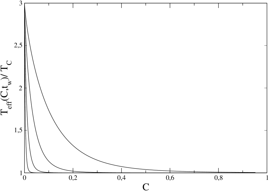
   From the explicit expressions for $f_{C}(x,y)$ and $f_{R}(x,y)$ in the critical quenches follows

   $$T_{eff}(t,t_{w},t_{0}) = F(x,y)$$ (112)

   $$= dT_{C}\left\{(x+y)\int_{0}^{1}dzz^{d/2-2}(x+1-2z+y)^{-1-d/2}\right.$$ (113)

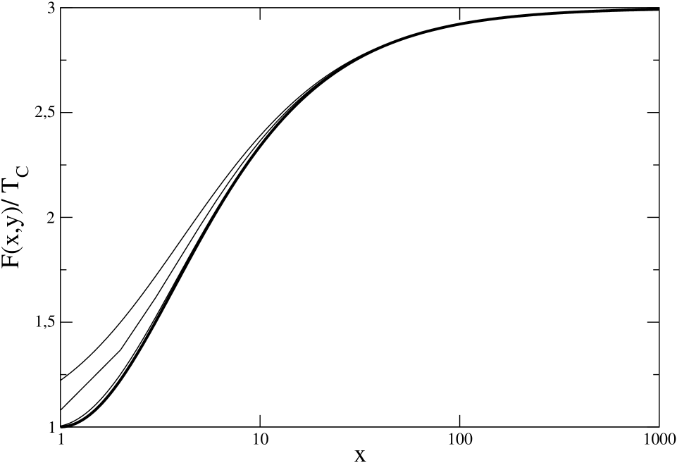
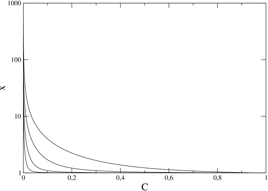
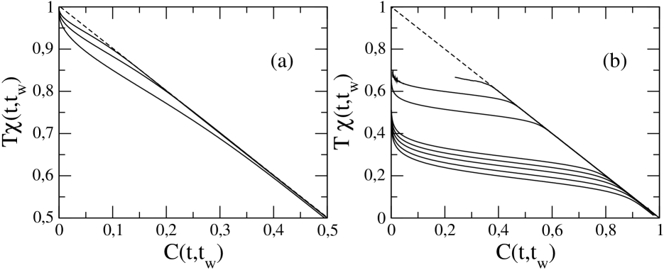
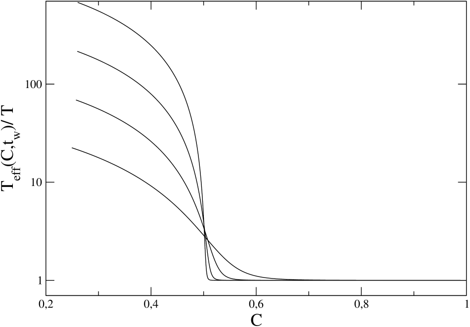
   $$- \left.{1\over 2}\int_{0}^{1}dzz^{d/2-2}(x+1-2z+y)^{-d/2}\right\}(x-1+y)^{d/2}.$$ (114)

   Evaluating numerically the right hand side, as $y\rightarrow 0$ the curve $F(x,y)$ approaches (Fig.3) the limit function $F(x,0)$ rising from $F(1,0)=T_{C}$ to $T_{\infty}=\lim_{x\to\infty}F(x,0)=T_{C}/X_{\infty}$, where $X_{\infty}=(d-2)/d$ [35]. Similarly, carrying out numerically the inversion of Eq. (103), the function $x=f_{C}^{-1}(t_{w}^{b}C,y)$ shows (Fig.4) the approach to the singular behavior (54) in the limit $y\rightarrow 0$. The parametric plot in Fig.5 displays the approach of $\widehat{T}(C,t_{w})$ toward ${\cal T}(C)$ of the form of Eq. (57) as $t_{w}\rightarrow\infty$, which can be very slow if $b$ is small. With the purpose of comparing further down with data for the XY model, in Fig.6 we have also shown the parametric plot of the ZFC susceptibility. This has been obtained by plotting $\chi(t,t_{w})$ against $C(t,t_{w})$ for fixed $t_{w}$ in two different cases: in panel (a), with $d=2.5$ corresponding to $b=0.25$, the approach to the asymptotic linear plot (60) is evident, while in panel (b), with $d=2.06$ corresponding to the much smaller value $b=0.03$, there is a much longer preasymptotic regime preceding the onset of the linear behavior.

2. Quench below the critical line

   Using Eqs. (107) and (109) we may rewrite Eq. (37) as

   $$T_{eff}(t,t_{w},t_{0})=Tx^{-d/4}+t_{w}^{d/2-1}F(x,y)(1-x^{-d/4})$$ (115)

   where

   $$F(x,y)=M^{2}(8\pi)^{d/2}{d\over 4}{x^{d/4}\over(x^{d/4}-1)}\left({x-1+y\over x+1+y}\right)^{1+d/2}.$$ (116)

   In Fig.7 we have plotted $T_{eff}(t,t_{w},t_{0})$ against the exact $C(t,t_{w},t_{0})$ obtaining $\widehat{T}(C,t_{w})$, which shows the approach toward the form (72) of ${\cal T}(C)$ as $t_{w}$ grows.

3. Quench to $T=0$ with $d=d_{L}$

   At $d=2$ and $T=0$, the second term in Eq. (84) vanishes and $b_{\sigma}=0$, yielding

   $$C(x,y)=2x^{1/2}(x+1+y)^{-1}$$ (117)

   while from Eqs. (115) and (116)

   $$T_{eff}(t,t_{w},t_{0})=(4\pi)\left({x-1+y\over x+1+y}\right)^{2}.$$ (118)

   Letting $y\rightarrow 0$ and eliminating $x$ between the above two equations we obtain the explicit non trivial expression

   $${\cal T}(C)=(4\pi)\left({1-C^{2}+\sqrt{1-C^{2}}\over 1+\sqrt{1-C^{2}}}\right)^{2}$$ (119)

   plotted in Fig.2c. We recall that the specific form of the function ${\cal T}(C)$ in the quench to $(d_{L},T=0)$ is nonuniversal.

VII XY model

In the XY model the phase diagram of Fig.1 includes the KT line and, as anticipated in the Introduction, in the $d=2$ case the behavior of ${\cal T}(C)$ for $0<T\leq T_{KT}$ is expected to be given by Eq. (57). This is hard to detect from existing data, since the small values of $b=\eta(T)/z$ at the temperatures used in [39, 40] would require to reach huge values of $t_{w}$ in order to observe the approach to (57). In Ref. [39] data are presented for the ZFC susceptibility. According to Eq. (59) asymptotically one should see the approach to the linear parametric plot (60), as illustrated in Fig.6a for the large-$N$ model. The data in Fig.10 of Ref. [39] seem to be far from this behavior and, indeed, in [39] these data have been regarded as reminiscent of the non trivial parametric plot in the $d=3$ Edwards-Anderson model. However, we believe that the non trivial pattern displayed by these data must be attributed to the large preasymptotic effect due to the small value of $b=\eta(T)/z=0.03$. Indeed, the pattern displayed by $\chi(C,t_{w})$ in Fig.10 of Ref. [39] is strikingly similar to the one in Fig.6b for the critical quench in the large-$N$ model, despite the fact that in the large-$N$ model there is no KT transition. The data in Fig.6b have been generated in order to reproduce the same value of $b$ in the quench of the XY model considered in [39].

It would be interesting to have data for the XY model quenched at $d_{L}$ and $T=0$, where, according to the general argument of section III, $\chi(C)$ is expected to display the non trivial behavior discussed in section IV.

In the $d=3$ case in Ref. [41], the parametric plots of the FDR

$$X(C)=\lim_{t_{w}\to\infty}{T\over\widehat{T}_{eff}(C,t_{w})}={T\over{\cal T}(C)}$$ (120)

are presented in the quenches to and below $T_{C}$. The data display the approach to the asymtotic parametric forms

$$X(C)=\left\{\begin{array}[]{ll}X_{\infty}=T_{C}/T_{\infty}\qquad$for$\qquad C=0\\ 1\qquad$for$\qquad 0<C\leq 1\end{array}\right.$$ (123)

in the quench to $T_{C}$ and

$$X(C)=\left\{\begin{array}[]{ll}0\qquad$for$\qquad C<M^{2}\\ 1\qquad$for$\qquad M^{2}\leq C\leq 1\end{array}\right.$$ (126)

in the quench below $T_{C}$, which correspond to Eqs. (57) and (72) for ${\cal T}(C)$.

Furthermore, in the $d=3$ model of particular interest is the measurement of the exponent $a$ below $T_{C}$. The value $a=1/2$ has been obtained both from the ZFC susceptibility [17] and from the direct mesurement of $R(t,t_{w},t_{0})$ [41]. This value gives additional and clearcut evidence in favour Eq. (83), which, in fact, predicts $a=1/2$ when $d=3$ and the order parameter is non conserved $(z=2)$ and vectorial $(n=2,d_{U}=4)$. Conversely, the conjecture [32] relating $a$ to the density of defects, would predict $a=1$, since in the XY model, with a vectorial order parameter, the density of defects goes like $t^{-1}$ [10, 42].

VIII Conclusions

In this paper we have overviewed the behavior of the effective temperature in the slow relaxation processes arising when systems, like a ferromagnet, with a simple pattern of ergodicity breaking in the low temperature state, are quenched from high temperature to or below $T_{C}$. On the basis of very general assumptions on the scaling properties of the autocorrelation and response functions, we have derived the scaling behavior of the effective temperature, which allows to account in a unified way for the different patterns displayed by ${\cal T}(C)$ in the different regions of the phase diagram. The primary results are i) in the critical quenches with $T_{C}>0$, as a consequence of $a=b>0$, ${\cal T}(C)$ displays always the form (57), which is trivial in the sense that ${\cal T}(C)=T_{C}$ except for the limiting value $T_{\infty}$ of Godrèche and Luck at $C=0$. In particular, this implies that also in the $d=2$ XY model quenched to $0<T\leq T_{KT}$ ${\cal T}(C)$, and the equivalent parametric representations of the FDR or the ZFC susceptibility, must be trivial. The non trivial behavior reported in ref. [39], then, must be regarded as preasymptotic. ii) The non trivial form of ${\cal T}(C)$ in the quenches to $(d_{L},T=0)$ requires $a=0$. Since, due to weak ergodicity breaking, this process cannot be regarded as the continuation to $T_{C}=0$ of the critical quenches, $a=0$ cannot be explained on the basis of Eq. (11). Rather, the exponent $a$ in the quenches below $T_{C}$ must be expected to have a dimensionality dependence such that $\lim_{d\to d_{L}}a=0$. The phenomenological formula (83) fits quite well within this framework, although a deeper theoretical understanding of the problem is needed in order to put it on firmer grounds.

Acknowledgements

We wish to thank Pasquale Calabrese, Silvio Franz and Mauro Sellitto for very useful discussions. This work has been partially supported by MURST through PRIN-2002.

FIG. 1.: Schematic phase diagram in the $d-T$ plane with the critical line $T_{C}(d)$ and the Kosterlitz-Thouless line for the 2d XY model.

FIG. 2.: Parametric plot of the effective temperature ${\cal T}(C)$: (a) quench to $T_{C}>0$, (b) quench to $T<T_{C}$ (c) quench to $(d_{L},T=0)$. Panel (c) has been generated plotting the explicit form of ${\cal T}(C)$ given by Eq. (119) in the large-$N$ model.

FIG. 3.: Approach to the limiting curve $F(x,0)$ (thick line) for $t_{w}=1,2,10,100$ (top to bottom) in the critical quench of the 3d large-$N$ model.

FIG. 4.: Approach to the limiting function $x(C)$ of Eq. (54) for $t_{w}=10,10^{2},10^{3},10^{4}$ (top to bottom) in the critical quench of the 3d large-$N$ model.

FIG. 5.: Approach of $\widehat{T}_{eff}(C,t_{w})$ toward ${\cal T}(C)$ of the form of Eq. (57) for $t_{w}=10,10^{2},10^{3},10^{4}$ (top to bottom) in the critical quench of the 3d large-$N$ model.

FIG. 6.: Parametric plot of the ZFC susceptibility in the critical quench of the large-$N$ model: (a) $d=2.05$, $t_{w}=10^{2},10^{3},10^{4}$ (bottom to top), (b) $d=2.06$, $t_{w}=10^{2},3\times 10^{2},10^{3},3\times 10^{3},10^{4},10^{6},10^{9},10^{12}$ (bottom to top).

FIG. 7.: Approach of $\widehat{T}_{eff}(C,t_{w})$ toward ${\cal T}(C)$ of the form of Eq. (72) for $t_{w}=10^{2},10^{3},10^{4},10^{5}$ (bottom to top) in the quench to $T=T_{c}/2$ of the 3d large-$N$ model.

REFERENCES

- [1] For a recent review see Cugliandolo L F, Dynamics of glassy systems, [cond-mat/0210312].
- [2] Cugliandolo L F and Kurchan J, Analytical solution of the off-equilibrium dynamics of a long-range spin-glass model, 1993 Phys.Rev.Lett. 71 173 [cond-mat/9303036]; On the out-of-equilibrium relaxation of the Sherrington-Kirkpatrick model, 1994 J.Phys.A: Math.Gen. 27 5749 [cond-mat/9311016].
- [3] Crisanti A and Ritort F, Violation of the fluctuation-dissipation theorem in glassy systems: basic notions and the numerical evidence, 2003 J.Phys.A:Math.Gen. 36 R181 [cond-mat/0212490].
- [4] Cugliandolo L F, Kurchan J and Peliti L, Energy flow, partial equilibration, and effective temperatures in systems with slow dynamics, 1997 Phys.Rev. E 55 3898 [cond-mat/9611044].
- [5] Sollich P, Fielding S and Mayer P, Fluctuation-dissipation relations and effective temperatures in simple non-mean field systems, 2002 J.Phys:Cond.Matt. 14 1683 [cond-mat/0111241].
- [6] Calabrese P and Gambassi A, On the definition of a unique effective temperature for non-equilibrium critical systems [cond-mat/0406289].
- [7] Franz S, Mézard M, Parisi G and Peliti L, Measuring equilibrium properties in aging systems, 1998 Phys.Rev.Lett. 81 1758 [cond-mat/9803108]; The response of glassy systems to random perturbations: a bridge between equilibrium and off-equilibrium, 1999 J.Stat.Phys. 97 459 [cond-mat/9903370].
- [8] Cugliandolo L F, Effective temperatures out of equilibrium [cond-mat/9903250].
- [9] Parisi G, Ricci-Tersenghi F and Ruiz-Lorenzo J J, Generalized off-equilibrium fluctuation-dissipation relations in random Ising systems, 1999 Eur.Phys.J. B 11 317 [cond-mat/9811374].
- [10] Bray A J, Theory of phase-ordering kinetics, 1994 Adv.Phys. 43 357.
- [11] Godrèche C and Luck J M, Nonequilibrium critical dynamics of ferromagnetic spin systems, 2002 J.Phys.:Cond. Matt. 14 1589 [cond-mat/0109212].
- [12] Calabrese P and Gambassi A, Ageing properties of critical systems [cond-mat/0410357].
- [13] Lippiello E and Zannetti M, Fluctuation dissipation ratio in the one dimensional kinetic Ising model, 2000 Phys.Rev. E 61 3369 [cond-mat/0001103].
- [14] Godrèche C and Luck J M, Response of non-equilibrium systems at criticality: exact results for the Glauber-Ising chain, 2000 J.Phys.A: Math.Gen. 33 1151 [cond-mat/9911348].
- [15] Corberi F, Lippiello E and Zannetti M, Slow relaxation in the large model for phase ordering, 2002 Phys.Rev. E 65 046136 [cond-mat/0202091].
- [16] Corberi F, Lippiello E and Zannetti M, On the connection between off-equilibrium response and statics in non disordered coarsening systems, 2001 Eur.Phys.J.B 24 359 [cond-mat/0110651]; Interface fluctuations, bulk fluctuations, and dimensionality in the off-equilibrium response of coarsening systems, 2001 Phys.Rev. E 63 06150629 [cond-mat/0007021].
- [17] Corberi F, Castellano C, Lippiello E and Zannetti M, Generic features of the fluctuation dissipation relation in coarsening systems, 2004 Phys.Rev. E 70 017103 [cond-mat/0311046].
- [18] Corberi F, Lippiello E and Zannetti M, Comment on “Aging, phase ordering and conformal invariance”, 2003 Phys.Rev.Lett. 90 099601 [cond-mat/0211609]; Scaling of the linear response function from zero-field-cooled and thermoremanent magnetization in phase-ordering kinetics, 2003 Phys.Rev. E 68 046131 [cond-mat/0307542].
- [19] Mazenko G F, Valls O T and Zhang F C, Kinetics of first-order phase transitions: Monte Carlo simulations, renormalization-group methods, and scaling for critical quenches, 1985 Phys.Rev. B 31, 4453; Bray A J, Renormalization-group approach to domain-growth scaling, 1990 Phys.Rev. B 41 6724.
- [20] Hohenberg P C and Halperin B I, Theory of dynamic critical phenomena, 1977 Rev.Mod.Phys. 49 435.
- [21] For a review see Coniglio A, Geometrical approach to phase transitions in frustrated and unfrustrated systems, 2000 Physica A 281 129.
- [22] Kosterlitz J M, Thouless D J, Ordering, metastability and phase transitions in two-dimensional systems,1973 J. Phys.C 6, 1181.
- [23] Bouchaud J P, Cugliandolo L F, Kurchan J and Mézard M, Out of equilibrium dynamics in spin glasses and other glassy systems, in Spin Glasses and Random Fields edited by A.P.Young (World Scientific, Singapore, 1997) [cond-mat/9702070].
- [24] Janssen H K, Schaub B and Schmittmann B, New universal short-time scaling behavior of critical relaxation processes, 1989 Z.Phys. B 73 539.
- [25] Mazenko G F, Response functions in phase-ordering kinetics, 2004 Phys.Rev. E 69 016114 [cond-mat/0308169].
- [26] Henkel M, Phenomenology of local scale invariance: from conformal invariance to dynamical scaling, 2002 Nucl.Phys. B 641 405 [hep-th/0205256]; Henkel M, Pleimling M, Godrèche C and Luck J M, Aging, phase ordering and conformal invariance, 2001 Phys.Rev.Lett. 87 265701 [hep-th/0107122].
- [27] Henkel M, Paessens M and Pleimling M, Scaling of the linear response in simple aging systems without disorder, 2004 Phys.Rev. E 69 056109 [cond-mat/0310761].
- [28] Berthier L, Barrat J L and Kurchan J, Response function of coarsening systems, 1999 Eur.Phys.J.B 11 635 [cond-mat/9903091].
- [29] Lippiello E, Corberi F and Zannetti M, Off-equilibrium generalization of the fluctuation dissipation theorem for Ising spins and measurement of the linear response function [cond-mat/0407523].
- [30] For systems with vector order parameter there is not, as of yet, enough information, analytical or numerical, to conjecture the general form of the response function.
- [31] The equivalent formula for the FDR was derived in Ref. [11].
- [32] Barrat A, Monte-Carlo simulations of the violation of the fluctuation-dissipation theorem in domain growth processes, 1998 Phys.Rev.E 57 3629 [cond-mat/9710069].
- [33] In the Ohta-Jsnow-Kawaski approximation . A possible origin of the discrepancy with found in the simulations of scalar systems is discussed in [16].
- [34] Cugliandolo L F and Dean D S, Full dynamical solution for a spherical spin glass model, 1995 J.Phys.A:Math.Gen. 28 4213 [cond-mat/9502075].
- [35] Godrèche C and Luck J M, Response of non-equilibrium systems at criticality: ferromagnetic models in dimension two and above, 2000 J.Phys A. Math.Gen. 33 9141 [cond-mat/0001264].
- [36] Zippold W, Khun R and Horner H, Non-equilibrium dynamics of simple spherical spin models, 2000 Eur.Phys.J. B 13 531 [cond-mat/9904329].
- [37] Franz S and Virasoro M A, Quasi-equilibrium interpretation of ageing dynamics, 2000 J.Phys.A:Math.Gen. 33 891 [cond-mat/9907438].
- [38] Mazenko G F and Zannetti M, Growth of order in a sytem with continous symmetry, 1984 Phys.Rev.Lett. 53 2106; Instability, spinodal decomposition and nucleation in a system with continous symmetry, 1985 Phys.Rev.B 32 4565.
- [39] Berthier L, Holdsworth P C W and Sellitto M, Nonequilibrium critical dynamics of the two-dimensional XY model, 2001 J.Phys.A:Math.Gen. 34 1805 [cond-mat/0012194].
- [40] Abriet S and Karevski D, Off equilibrium dynamics in 2d-XY system [cond-mat/0309342].
- [41] Abriet S and Karevski D, Off equilibrium dynamics in the 3d-XY system [cond-mat/0405598].
- [42] Blundell R E and Bray A J, Phase-ordering dynamics of the O(n) model: exact predictions and numerical results, 1994 Phys.Rev.E 49 4925 [cond-mat/9310075].