4-pole analysis of the two-dimensional Hubbard model

Abstract

The electronic states of the two-dimensional Hubbard model are investigated by means of a 4-pole approximation within the Composite Operator Method. In addition to the conventional Hubbard operators, we consider other two operators, which come from the hierarchy of the equations of motion. These operators carry information regarding surrounding spin and charge configurations. By means of this operatorial basis, we can study the physics related to the energy scale $J=4t^{2}/U$. Results present, in addition to the main two bands, a quasi-particle peak at the Fermi level, shadow bands and band flatness at ($\pi$, 0) point.

, ,

The main gross feature of the Hubbard model is the splitting of the band with the formation of a gap of the order $U$. This physics can be well understood in terms of the two Hubbard operators, which mainly describe the two Hubbard sub-bands. However, in order to catch low-energy features related to the energy scale $J=4t^{2}/U$, it is necessary to take into account higher-order operators, which carry information regarding nearest-neighbor spin and charge correlation effects. Along this line, we analyze the Hubbard model by means of a 4-pole approximation within the Composite Operator Method [1, 2, 3, 4]. In addition to the conventional Hubbard operators, we consider other two operators that come from the hierarchy of the equations of motion. The resulting band structure will be much richer than the 2-pole one.

The two-dimensional Hubbard Hamiltonian reads as follows,

$$H=\sum_{\mathbf{ij}\sigma}(t_{\mathbf{ij}}-\mu\delta_{\mathbf{ij}})c^{\dagger}_{\sigma}(i)c_{\sigma}(j)+U\sum_{\mathbf{i}}n_{\uparrow}(i)n_{\downarrow}(i),$$ (1)

where $c^{\dagger}_{\sigma}(i)$ and $c_{\sigma}(i)$ are creation and annihilation operators of electrons with spin $\sigma$ at the site $\mathbf{i}\ [i=(\mathbf{i},t)]$, respectively. $n_{\sigma}(i)=c^{\dagger}_{\sigma}(i)c_{\sigma}(i)$, $\mu$ is the chemical potential, $t_{\mathbf{ij}}=-4t\alpha_{\mathbf{ij}}$, $\alpha[{\bf k}]=\mathcal{F}[\alpha_{\mathbf{ij}}]=\frac{1}{2}(\cos(k_{x}a)+\cos(k_{y}a))$, $a$ is the lattice constant, $\mathcal{F}$ is the Fourier transform, $U$ is the on-site Coulomb repulsion. We define the following operatorial basis,

$$\psi_{A\sigma}(i)=\left(\begin{array}[]{l}\xi_{\sigma}(i)\\ \eta_{\sigma}(i)\end{array}\right).$$ (2)

$\xi_{\sigma}(i)=c_{\sigma}(i)\left(1-n_{-\sigma}(i)\right)$ and $\eta_{\sigma}(i)=c_{\sigma}(i)n_{-\sigma}(i)$ describe the transitions $n(i)=0\leftrightarrow 1$ and $1\leftrightarrow 2$, respectively. The equations of motion of $\psi_{A\sigma}(i)$ give

$$\left\{\begin{array}[]{l}\displaystyle i\frac{\partial}{\partial t}\xi_{\sigma}(i)=-\mu\xi_{\sigma}(i)-4t\left[c^{\alpha}_{\sigma}(i)+\pi_{\sigma}(i)\right]\vspace*{1mm}\\ \displaystyle i\frac{\partial}{\partial t}\eta_{\sigma}(i)=(-\mu+U)\eta_{\sigma}(i)+4t\pi_{\sigma}(i).\end{array}\right.$$ (3)

where $\pi_{\sigma}(i)=-n_{-\sigma}(i)c^{\alpha}_{\sigma}(i)+c^{\dagger}_{-\sigma}(i)c_{\sigma}(i)c^{\alpha}_{-\sigma}(i)+c_{\sigma}(i)c^{\alpha\dagger}_{-\sigma}(i)c_{-\sigma}(i)$ with $c^{\alpha}_{\sigma}(i)=\sum_{\bf j}\alpha_{\bf ij}c_{\sigma}({\bf j},t)$. Now, we divide $\pi_{\sigma}(i)$ into two operators $\pi_{\sigma}(i)=\xi_{s\sigma}(i)+\eta_{s\sigma}(i)$ in the same manner as we have done with $c_{\sigma}(i)=\xi_{\sigma}(i)+\eta_{\sigma}(i)$. Then, we define a new operator set

$$\psi_{B\sigma}(i)=\left(\begin{array}[]{l}\xi_{s\sigma}(i)\\ \eta_{s\sigma}(i)\end{array}\right)$$ (4)

with

$$\begin{array}[]{l}\xi_{s\sigma}(i)=-n_{-\sigma}(i)\xi^{\alpha}_{\sigma}(i)+c^{\dagger}_{-\sigma}(i)c_{\sigma}(i)\xi^{\alpha}_{-\sigma}(i)\\ \hskip 39.83385pt+c_{\sigma}(i)\eta^{\alpha\dagger}_{-\sigma}(i)c_{-\sigma}(i)\vspace*{1mm}\\ \eta_{s\sigma}(i)=-n_{-\sigma}(i)\eta^{\alpha}_{\sigma}(i)+c^{\dagger}_{-\sigma}(i)c_{\sigma}(i)\eta^{\alpha}_{-\sigma}(i)\\ \hskip 39.83385pt+c_{\sigma}(i)\xi^{\alpha\dagger}_{-\sigma}(i)c_{-\sigma}(i).\end{array}$$ (5)

It is worth mentioning that $\psi_{B\sigma}(i)$ describes two-site composite excitations [5] as they carry information of surrounding spin and charge configurations, and are eigenoperators of the interaction term as $\xi_{\sigma}(i)$ and $\eta_{\sigma}(i)$.

In the present paper, we choose as operatorial basis

$$\psi_{\sigma}(i)=\left(\begin{array}[]{l}\psi_{A\sigma}(i)\\ \psi_{B\sigma}(i)\end{array}\right).$$ (6)

Within the Composite Operator Method, once we choose a $n$-component spinorial basis $\psi$, the equations of motion take the general form

$$i\frac{\partial}{\partial t}\psi(i)=\sum_{\bf j}\epsilon({\bf i},{\bf j})\psi({\bf j},t)+\delta j(i)$$ (7)

where $\epsilon({\bf k})=m({\bf k})I^{-1}({\bf k})$ is $n\times n$ matrix as $I({\bf k})=\mathcal{F}\langle\{\psi({\bf i},t),\psi^{\dagger}({\bf j},t)\}\rangle$ and $m({\bf k})=\mathcal{F}\langle\{i\frac{\partial}{\partial t}\psi({\bf i},t),\psi^{\dagger}({\bf j},t)\}\rangle$. If we neglect $\delta j$ we obtain a pole structure for the Green’s function

$$G(\omega,{\bf k})=\sum_{i=1}^{n}\frac{\sigma_{i}({\bf k})}{\omega-E_{i}({\bf k})}.$$ (8)

The 2-pole solution with $\psi=\psi_{A}$ have been discussed in detail in Refs. [2, 3]. In the present paper, we analyze a 4-pole solution by means of the basis (6). According to this, we have

$$I({\bf k})=\left(\begin{array}[]{cc}I_{AA}({\bf k})&I_{AB}({\bf k})\\ I_{AB}({\bf k})&I_{BB}({\bf k})\\ \end{array}\right)$$ (9)

$$\epsilon({\bf k})=\left(\begin{array}[]{cc}\epsilon_{AA}({\bf k})&\epsilon_{AB}({\bf k})\\ \epsilon_{BA}({\bf k})&\epsilon_{BB}({\bf k})\\ \end{array}\right)$$ (10)

The main difficulty of the present formulation is the evaluation of $I_{BB}({\bf k})$ and $\epsilon_{BB}({\bf k})$. The other elements can be simply computed either explicitly or in terms of those latter. For $I_{BB}({\bf k})$, we calculate anticommutators explicitly and decouple the higher-order correlation functions preserving particle-hole symmetry and hermiticy. For $\epsilon_{BB}({\bf k})$, we use the simplified equations of motion discussed in Ref. [5],

$$\begin{array}[]{l}i\frac{\partial}{\partial t}\xi_{s\sigma}(i)\simeq-\mu\xi_{s\sigma}(i)+4t\left[\frac{1}{2}\eta_{\sigma}(i)+\xi^{\alpha}_{s\sigma}(i)+2\eta^{\alpha}_{s\sigma}(i)\right]\vspace*{1mm}\\ i\frac{\partial}{\partial t}\eta_{s\sigma}(i)\simeq(-\mu+U)\eta_{s\sigma}(i)+4t\left[\frac{1}{4}\eta_{\sigma}(i)+\xi^{\alpha}_{s\sigma}(i)\right],\end{array}$$ (11)

where we neglect terms that give diffusion processes over three sites. This procedure simply gives $\epsilon_{BB}({\bf k})$ by inspection. The correlation functions appearing in the $I$ and $\epsilon$ are self-consistently determined by means of Green’s function and the local algebra constraints [4].

In Fig. 1, we present the density of states and the dispersion relation. It is worth noticing that the above formulation is applicable in any dimension. In addition to the main Hubbard band structure, our results show a coherent peak around the Fermi level and shadow bands originated by the antiferromagnetic correlations. The details of formulae and a more extended analysis will be presented elsewhere.

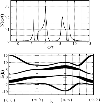
Figure 1: The density of states (top) and the dispersion relation (bottom) for $U=8t$, $n=0.9$ and $T=0.01t$. The width of dispersion line gives the intensity of peak.

References

[1] S. Ishihara, H. Matsumoto, S. Odashima, M. Tachiki, F. Mancini,
Phys. Rev. B49 (1994) 1350.
[2] F. Mancini, S. Marra, H. Matsumoto, Physica C244 (1995) 49;
Physica C250 (1995) 184.
[3] A. Avella, F. Mancini, D. Villani, L. Siurakshina,
V.Yu. Yushankhai, Int. J. Mod. Phys. B 12 (1998) 81.
[4] F. Mancini, A. Avella, Eur. Phys. J. B 36 (2003) 37.
[5] A. Avella, F. Mancini, S. Odashima, J. Magn. Magn. Mater. 272-276 (2004) E311.