Overcoming the critical slowing down of flat-histogram Monte Carlo simulations: Cluster updates and optimized broad-histogram ensembles

Abstract

We study the performance of Monte Carlo simulations that sample a broad histogram in energy by determining the mean first-passage time to span the entire energy space of $d$-dimensional ferromagnetic Ising/Potts models. We first show that flat-histogram Monte Carlo methods with single-spin flip updates such as the Wang-Landau algorithm or the multicanonical method perform sub-optimally in comparison to an unbiased Markovian random walk in energy space. For the $d=1,2,3$ Ising model, the mean first-passage time $\tau$ scales with the number of spins $N=L^{d}$ as $\tau\propto N^{2}L^{z}$. The critical exponent $z$ is found to decrease as the dimensionality $d$ is increased. In the mean-field limit of infinite dimensions we find that $z$ vanishes up to logarithmic corrections. We then demonstrate how the slowdown characterized by $z>0$ for finite $d$ can be overcome by two complementary approaches – cluster dynamics in connection with Wang-Landau sampling and the recently developed ensemble optimization technique. Both approaches are found to improve the random walk in energy space so that $\tau\propto N^{2}$ up to logarithmic corrections for the $d=1,2$ Ising model.

I Introduction

Recently, Wang and Landau wl1 ; wl2 introduced a Monte Carlo (MC) algorithm that simulates a biased random walk in energy space, systematically estimates the density of states, $g(E)$, and iteratively samples a flat histogram in energy. The bias depends on the total energy $E$ of a configuration and is defined by a statistical ensemble with weights $w(E)=1/g(E)$. The idea is that the probability distribution of the energy, $p(E)=w(E)g(E)$, will eventually become constant, producing a flat energy histogram. The algorithm has been successfully applied to a wide range of systems gubernatis .

One measure of the performance of the Wang-Landau algorithm and other broad-histogram algorithms is the mean first-passage time $\tau$, which we define to be the number of MC steps per spin for the system to go from the configuration of lowest energy to the configuration of highest energy. This time has been called the tunneling time or round-trip time in earlier work tt ; EnsembleOptimization . This time is the relevant scale for sampling the entire energy space. Because the number of possible energy values in the Ising model scales linearly with the number of spins $N=L^{d}$, where $d$ is the spatial dimension, we might expect from a simple random walk argument that $\tau\propto N^{2}$. However, it was recently shown that for flat-histogram algorithms $\tau$ scales as

$$\tau\sim N^{2}L^{z},$$ (1)

where the exponent $z$ is a measure of the deviation of the random walk from unbiased Markovian behavior tt . In analogy to the dynamical critical exponent for canonical simulations, the exponent $z$ quantifies the critical slowing down for the simulated flat-histogram ensemble and the chosen local update dynamics EnsembleOptimization . For the Ising model on a square lattice it was shown in Ref. tt that $z\approx 0.74$.

In this paper, we determine the performance of the single-spin flip Wang-Landau algorithm for the ferromagnetic Ising model as a function of the dimension $d$. We find that the exponent $z$ is a decreasing function of $d$. By using Monte Carlo simulations we determine that $z\approx 1.814$, 0.743, and 0.438 for $d=1$, 2, and 3, respectively (see Sec. II.1). In the mean-field limit of infinite dimension we find that $z=0$ using Monte Carlo simulations and analytic methods (Sec. II.2). To round out our examination of the single-spin flip algorithm, we also estimate $z$ for the $q=10$ and $q=20$ Potts model in $d=2$ (see Sec. II.3).

We then discuss two complementary approaches that overcome the critical slowing down of the single-spin flip flat-histogram algorithm. In Sec. III we demonstrate that flat-histogram MC simulations can be speeded up by changing the spin dynamics, that is, by using cluster updates instead of local updates janke ; kawashima . Alternatively, we apply the recently developed ensemble optimization technique EnsembleOptimization to change the simulated statistical ensemble and show that by sampling an optimized histogram instead of a flat-histogram, the critical slowing down of the single-spin flip simulation can also be eliminated (Sec. IV). For the Ising model in one and two dimensions we find that both approaches result in optimal $N^{2}$-scaling of the random walk up to logarithmic corrections.

II Performance of flat-histogram algorithms with local updates

In this section we study the performance of the single-spin flip flat-histogram algorithm by measuring the mean first-passage time for the $d=1$, 2, 3 and mean-field Ising models and the $q$-state Potts model in $d=2$.

II.1 The mean first-passage times for the Ising model in $\mathbf{d=1}$, 2, and 3

For the $d=1$ Ising model, the mean first-passage time time was calculated using the exact density of states and 50,000 MC measurements for each value of $N$. A power-law fit in the range $70\leq N\leq 500$ gives $z=1.814\pm 0.014$ as shown in Fig. 1. However, there is some curvature in the data which indicates a deviation from this power-law scaling and the effective value of $z$ seems to increase as larger system sizes are taken into account. Thus we cannot eliminate the possibility that $z=2$.

A crude argument that $z\leq 2$ comes from considering the two lowest states of a spin chain. The ground state has all spins aligned, and the first excited state has a single misaligned domain bounded by two domain walls. The distance between the domain walls is typically the order of $L$, the linear dimension of the system. For single spin flip dynamics the domain walls perform a random walk so that the typical number of sweeps required to make the transition from the first excited state to the ground state scales as $L^{2}$. If this diffusion time were to hold for all energies, the result would be $z=2$. However, for higher energy states the domain wall diffusion time becomes smaller, so $z=2$ is an upper bound for the $d=1$ Ising model.

Figure 1: Scaling of the mean first-passage time in the energy interval $[-N,+N]$ for the flat-histogram random walker of the $d=1$ Ising model. The dashed line corresponds to a power-law fit in the range $70\leq N\leq 500$, which yields a critical exponent of $z=1.814\pm 0.014$.

The exact density states also was used for $d=2$ footnote1 . The combined results from Ref. tt and this work are shown in Fig. 2 where each data point represents a total of 50,000 measurements. A power-law fit of the critical exponent $z$ for $10\leq L\leq 64$ gives $z=0.743\pm 0.002$.

Figure 2: Scaling of the mean first-passage time in the energy interval $[-2N,+2N]$ for the flat-histogram random walker of the $d=2$ Ising model. The dashed line corresponds to a power-law fit, which yields $z=0.743\pm 0.002$.

For the $d=3$ Ising model the exact Ising density of states cannot be calculated exactly, except for very small systems. We first used the Wang-Landau algorithm wl1 ; wl2 to estimate the density of states. The criteria for the completion of each iteration in the determination of $g(E)$ was that each energy be visited at least five times and that the variance of the histogram be less than 10% of the mean. Because $g(E)$ is symmetric about $E=0$, the calculated values for $g(E)$ and $g(-E)$ were averaged. For each value of $N$, $g(E)$ was independently calculated ten times and then each $g(E)$ was used to obtain $\tau$ by averaging over 5,000 measurements. The results for the first-passage time $\tau$ were then averaged over ten independent runs. The results are shown in Fig. 3 and yield $z=0.438\pm 0.010$.

Figure 3: Scaling of the mean first-passage time in the energy interval $[-3N,+3N]$ for the flat-histogram random walker of the $d=3$ Ising model. The dashed line corresponds to a power-law fit for $L\geq 8$, which yields $z=0.743\pm 0.002$.

II.2 Mean-Field Ising model

The results of Sec. II.1 indicate that the value of $z$ decreases with increasing dimension. This dependence suggests that it would be interesting to compute $\tau$ for the Ising model in the mean-field limit. We consider the “infinite-range” Ising model for which every spin interacts with every other spin with an interaction strength proportional to $1/N$. In this system the energy $E$ and magnetization $M$ are simply related, and it is convenient to express the density of states in terms of the latter. For each value of $N$ we did 50,000 MC measurements of $\tau$ in the range $4\leq N\leq 8000$.

We also calculated $\tau$ from a master equation. Because flipping a spin changes the magnetization by $\pm 2$, the master equation takes the form (suitably modified near the extremes of $M=\pm N$)

$$P(M,t+1)= P(M,t)+T(M+2,M)\,P(M+2,t)$$

$$-[T(M,M+2)+T(M,M-2)]\,P(M,t)$$

$$+T(M-2,M)\,P(M-2,t),$$ (2)

where $P(M,t)$ is the probability that the system has magnetization $M$ at time $t$ and $T(M_{1},M_{2})$ is the probability of a transition from a state with magnetization $M_{1}$ to one with $M_{2}$. The transition probabilities $T$ are products of the probability of choosing a spin in the desired direction times the probability of accepting the flip. The latter is the Wang-Landau probability, $W(M_{1},M_{2})$, which is given by

$$W(M_{1},M_{2})=\min\Big{[}1,{{g(M_{1})}\over{g(M_{2})}}\Big{]}.$$ (3)

The probability of choosing a spin in the desired direction is determined as follows. In a transition in which the magnetization increases, a down spin must be chosen. The probability of choosing a down spin is the number of down spins, $N_{\downarrow}$, divided by the total number of spins,

$${N_{\downarrow}(M)\over N}={{N-M}\over{2\,N}}.$$ (4a)

Similarly, in a transition in which the magnetization decreases, an up spin must be chosen. The probability is

$${N_{\uparrow}(M)\over N}={{N+M}\over{2\,N}}.$$ (4b)

The transition probabilities can now be written as:

$$T(M+2,M) = {N_{\uparrow}(M+2)\over N}W(M+2,M)$$ (5a)

$$T(M,M+2) = {N_{\downarrow}(M)\over N}W(M,M+2)$$ (5b)

$$T(M-2,M) = {N_{\downarrow}(M-2)\over N}W(M-2,M)$$ (5c)

$$T(M,M-2) = {N_{\uparrow}(M)\over N}W(M,M-2)$$ (5d)

The Wang-Landau probability $W(M_{1},M_{2})$ can be simplified for this system in the following way: the density of states in terms of the magnetization is

$$g(M)={N\choose N_{\uparrow}}.$$ (6)

If $|M|$ increases in the transition, that is, $|M_{1}|<|M_{2}|$, then $W(M_{1},M_{2})=1$ because the ratio of the density of states exceeds unity. If $|M|$ decreases, there are two cases. For $M<0$, $N_{\uparrow}$ increases by $1$ and $M$ increases by 2, and we have

$$W(M,M+2)={{g(M)}\over{g(M+2)}}={{N\choose N_{\uparrow}}\over{N\choose{N_{\uparrow}+1}}}={{N+M+2}\over{N-M}}.$$ (7a)

If $$M>0 N_{\uparrow} M 2$$, decreases by 1 and decreases by , and

$$W(M,M-2)={g(M)\over g(M-2)}={{N\choose N_{\uparrow}}\over{N\choose N_{\uparrow}-1}}={N-M+2\over N+M}.$$ (7b)

Equations (3) and (7) can be combined into the following simple expression

$$W(M,M\pm 2)=\min\Big{[}1,{{N\pm M+2}\over N+|M|}\Big{]}.$$ (8)

To compute the mean first-passage time, we take the state with magnetization $N$ (the state with the highest magnetization) to be absorbing. The initial condition is

$$P(M,0)=\begin{cases}1&\text{$M=-N$}\\ 0&\text{otherwise}\;.\end{cases}$$ (9)

To compute $\tau$, we iterate Eq. (2) using Eqs. (5) and (7) and compute $\Delta P(N,t)$, the change in the value of $P(N,t)$ after each iteration $t$. The mean first-passage time is then given by

$$\tau=\sum_{t}t\,\Delta P(N,t).$$ (10)

A comparison of the distribution of first-passage times calculated from the master equation and from a direct simulation is shown in Fig. 4. As shown in Fig. 5, the scaling of the mean first-passage time with $N$ is consistent with $\tau/N^{2}\sim\ln N$. The fit includes both the master equation and simulation results.

Figure 4: Comparison of the distribution of first-passage times for the mean-field Ising model computed by iterating the master equation (line) and by direct simulation (points) for $N=32$. The master equation results were normalized to 50,000 MC estimates.

The logarithmic behavior of $\tau$ can be determined analytically from the transition rates using the first-passage time methods described in Ref. Redner . Let $t(m)$ be the mean first-passage time starting from magnetization $m=M/N$ and ending at the absorbing boundary $m=1$ with a reflecting boundary at $m=-1$. We seek $\tau=t(-1)$. The mean first-passage time satisfies,

$$t(m) = [t(m-\delta m)+\delta t]T_{-}(m)$$ (11)

$${}+[t(m+\delta m)+\delta t]T_{+}(m)$$

$${}+[t(m)+\delta t]T_{0}(m),$$

where $T_{-}(m)=T(M,M-2)$, $T_{+}(m)=T(M,M+2)$ are the transition probabilities, $T_{0}=1-T_{-}-T_{+}$ is the waiting probability, $\delta m=2/N$ is the magnetization step size, and $\delta t=1$ is the time unit for a step. Equation (11) can be cast in differential form by expanding $t(m)$ to second order in $\delta m$,

$$1+h(m)t^{\prime}(m)+f(m)t^{\prime\prime}(m)=0,$$ (12)

where

$$f(m)=(\delta m^{2}/2\delta t)[T_{+}(m)+T_{-}(m)],$$ (13)

and $h(m)=(\delta m/\delta t)[T_{+}(m)-T_{-}(m)]$. The absorbing boundary requires that

$$t(1)=0.$$ (14)

At the reflecting boundary, the transition to the left vanishes, $T_{-}(-1)=0$, and we have

$$t(-1) = [t(-1+\delta m)+\delta t]T_{+}(-1)$$ (15)

$${}+[t(-1)+\delta t][1-T_{+}(-1)].$$

If we expand Eq. (15) to first order in $\delta m$, we obtain the boundary condition

$$t^{\prime}(-1)=-\frac{\delta m}{2f(-1)},$$ (16)

where $f(-1)=(\delta m^{2}/2\delta t)T_{+}(m)$

The flat-histogram feature of the Wang-Landau method means that the random walk satisfies the simple detailed balance condition,

$$T_{+}(m) = T_{-}(m+\delta m)$$ (17a)

$$T_{-}(m) = T_{+}(m-\delta m).$$ (17b)

We expand the detailed balance conditions to first order in $\delta m$ and find a relation between the coefficients in Eq. (12),

$$h(m)=f^{\prime}(m),$$ (18)

with the result that Eq. (12) reduces to

$$1+f^{\prime}(m)t^{\prime}(m)+f(m)t^{\prime\prime}(m)=0.$$ (19)

If we take into account the reflecting boundary condition, the solution to the differential equation is

$$t(m)=\tau-\!\int_{-1}^{m}\frac{x+1+\delta m/2}{f(x)}dx,$$ (20)

where $\tau=t(-1)$ is the first-passage time we are seeking. We use the absorbing boundary condition to find that

$$\tau=\!\int_{-1}^{1}\frac{x+1+\delta m/2}{f(x)}dx.$$ (21)

Because $f(m)$ is an even function, the first term in the integrand vanishes. We substitute $\delta m=2/N$ and use Eq. (13) for $f(m)$ to obtain the leading behavior of $\tau$,

$$\tau=2N^{2}\!\int_{-1}^{1}\frac{1}{1-T_{0}(x)}dx.$$ (22)

From Eqs. (4), (5), and (8) we have that $T_{0}(m)=|m|-1/N$, which yields the desired result

$$\tau=2N^{2}\!\int_{-1}^{1}\frac{dm}{1-|m|+1/N}\sim N^{2}\log N.$$ (23)

Note that the integral can be interpreted as the average waiting time and that this average is dominated by the two boundaries.

Figure 5: Scaling of the mean first-passage time in the magnetization interval $[-N,+N]$ for the flat-histogram random walk of the mean-field Ising model. Note the linear scale on the $y$-axis. The $+$ symbol denotes the simulation results and $\times$ denotes results derived from the master equation. The dashed line corresponds to a logarithmic fit of the combined results for $L\geq 50$. The slope is found to be $0.977\pm 0.004$.

II.3 The Potts model

In Ref. EnsembleOptimization it was shown that the non-vanishing scaling exponent $z$ quantifies the critical slowing down of the flat-histogram simulation near a critical point. Most strikingly, this slowing down can be observed as a suppression of the local diffusivity of the flat-histogram random walker (see Sec. IV). The Ising model undergoes a second order phase transition. Here we extend our analysis to first-order phase transitions as is observed in $q$-state Potts models with $q>4$ on a square lattice.

Because the exact density of states is not known for the $q$-state Potts model, we follow the same procedure as for the Ising model in $d=3$ making use of the Wang-Landau algorithm. Based on these estimates for the density of states, we measured the mean first-passage time as a function of the linear system size $L$ as is illustrated in Fig. 6. For $q=10$ we find that the critical exponent $z$ becomes $z=0.786\pm 0.010$, which is close to our result for the $d=2$ Ising model thereby showing the close proximity of this weak first-order phase transition to a continuous phase transition. For the $q=20$ Potts model we find $z=0.961\pm 0.008$, illustrating increasing critical slowing down as the strength of the first-order transition increases. However, we cannot rule out exponential slowing down for even larger values of $q$ as was observed for multicanonical simulations of droplet condensation in the $d=2$ Ising model Neuhaus:2003 .

Figure 6: Scaling of the mean first-passage time in the energy interval $[-2N,0]$ for the flat-histogram random walk of the $d=2$, $q=10$ and $q=20$ Potts models. The dashed lines correspond to power-law fits for $L\geq 8$ and yield $z=0.786\pm 0.010$ and $z=0.961\pm 0.008$ for the $q=10$ and $q=20$ Potts models, respectively.

III Changing the dynamics:
Cluster Updates

In Sec. II we found that single-spin flip flat-histogram Monte Carlo simulations suffer from a critical slowing down, that is, $z>0$, for the Ising model in $d=1$, 2, and 3. The critical slowing down associated with single-spin flip algorithms near critical points in the canonical ensemble has been reduced by the introduction of cluster algorithms such as the Swendsen-Wang algorithm sw and the Wolff algorithm wolff . In this section we follow a similar approach and combine efficient cluster updates with flat-histogram simulations.

In conventional cluster algorithms sw ; wolff simulating the canonical ensemble, clusters of parallel spins are built up by adding aligned spins to the cluster with a probability $p(\beta)$, which explicitly depends on the temperature $\beta=1/T$. When simulating a broad-histogram ensemble in energy there is no explicit notion of temperature, and thus no straightforward analogue of a cluster algorithm. Recently, Reynal and Diep suggested a solution of this problem by using an estimate of the microcanonical temperature $\beta(E)=dS(E)/dE$ diep .

A complementary approach is to sample a broad-histogram ensemble using an alternative representation of the system’s partition function for which it is possible to genuinely introduce cluster updates. An example is the multibondic method introduced by Janke and Kappler janke which uses the Fortuin-Kasteleyn (FK) representation fk in the context of multicanonical sampling. Although the multibondic method performs local updates of the graph in the FK representation and cluster updates of the spin configurations, Yamaguchi and Kawashima were able to show that a global and rejection free update of the graph in the FK representation is possible kawashima . We will discuss methods based on graph representations in Sec. III.1.

The above methods can only be applied to Ising and Potts models. In Sec. III.2 we introduce a new representation using multigraphs that allows cluster updates for continuous spin models in the context of broad-histogram ensembles.

In the following we assume that the Hamiltonian of the system has the form

$$H[\sigma]=-\sum_{\langle ij\rangle}h_{ij}[\sigma_{i},\sigma_{j}]\;,$$ (24)

where $\sigma$ denotes the configuration of the system, $\sigma_{i}$ the spin of site $i$, and the sum is over all bonds $\langle ij\rangle$ that define the lattice of the system.

III.1 Graph representation

We first review the cluster methods based on an additional graph variable and present results showing that $z=0$ for multibondic flat-histogram simulations of Ising models. In the spin representation the canonical partition function of the Ising-Potts model is given by $Z=\sum_{\sigma}W_{\sigma}(\sigma)$, where the summation is over all spin configurations, and the weight of a spin configuration is $W_{\sigma}(\sigma)=e^{-\beta H[\sigma]}$.

The $q$-state Ising-Potts system also can be represented by a sum over all graphs $\omega$ that can be embedded into the lattice. The partition function is then

$$Z=\sum_{\omega}{W_{\omega}(\omega)},$$ (25)

and the weight of a graph $\omega$ is given by

$$W_{\omega}(\omega)=p^{n(\omega)}(1-p)^{n_{b}-n(\omega)}q^{c(\omega)}.$$ (26)

$n(\omega)$ is the number of of bonds in the graph $\omega$, $c(\omega)$ the number of connected components (counting isolated sites), and $n_{b}$ is the total number of bonds in the lattice. Because the graph $\omega$ can be viewed as a subgraph of the lattice, its bonds are sometimes referred to as “occupied bonds,” and the bond probability of the ferromagnetic Ising-Potts model with $h_{ij}[\sigma_{i},\sigma_{j}]=\delta_{\sigma_{i},\sigma_{j}}$ is given by fk

$$p(\beta)=1-e^{-\beta}.$$ (27)

A third representation of the Ising-Potts model is the spin-bond representation, which is employed in the Swendsen-Wang algorithm sw . In the spin-bond representation the system is characterized by both spins and bonds, with the requirement that a bond can be occupied only if it is satisfied, that is if the two spins connected by a bond in $\omega$ have the same value. In this representation the partition function is

$$Z=\sum_{\sigma,\omega}{W_{\sigma\omega}(\sigma,\omega)},$$ (28)

and the weight is given by

$$W_{\sigma\omega}(\sigma,\omega)=p^{n(\omega)}(1-p)^{n_{b}-n(\omega)}\Delta(\sigma,\omega),$$ (29)

where $\Delta(\sigma,\omega)=1$ if all occupied bonds are satisfied and zero otherwise.

It is natural to introduce a density of states for each of the three representations: For the spin representation in terms of the energy $E$, we write

$$g_{\sigma}(E)=\sum_{\sigma}\delta({H[\sigma]}-E).$$ (30)

For the bond representation in terms of the number of occupied bonds $n$ and number of clusters $c$, we have

$$g_{\omega}(n,c)=\sum_{\omega}\delta({n(\omega)}-n)\,\delta(c(\omega)-c).$$ (31)

And for the spin-bond representation in terms of the number of occupied bonds $n$, we write

$$g_{\sigma\omega}(n)=\sum_{\omega,\sigma}\delta({n(\omega)}-n)\,\Delta(\sigma,\omega).$$ (32)

The corresponding forms of the partition function are

$$Z =\sum_{E}{g_{\sigma}(E)\,e^{-\beta E}}$$ (spin) (33)

$$Z =\sum_{n,c}{g_{\omega}(n,c)\,p^{n}\,(1-p)^{n_{b}-n}\,q^{c}}$$ (bond) (34)

$$Z =\sum_{n}g_{\sigma\omega}(n)\,p^{n}\,(1-p)^{n_{b}-n}.$$ (spin-bond) (35)

The Wang-Landau algorithm can be applied in all three representations. As discussed in Sec. II, the spin representation has a relatively large value of $z$.

The bond representation generally requires a two-dimensional histogram, but for the $d=1$ Ising-Potts model, the number of clusters $c$ is completely determined by the number of occupied bonds $n$ and a one-dimensional histogram is sufficient. We simulated the $d=1$ Ising model in the bond representation and found that the mean first-passage time scales as $N^{2}\log L$, as shown in Fig. 7. It is noteworthy that the domain wall arguments used to explain the large value of $z$ in one dimension do not apply in the bond representation.

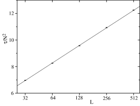
Figure 7: Scaling of the mean first-passage time applying cluster updates in the bond representation for the $d=1$ Ising model. Note the linear scale of the $y$-axis.

In higher dimensions $n$ does not determine $c$, and it is simpler to use the spin-bond representation. The resulting multibondic algorithm kawashima is very similar to the Swendsen-Wang algorithm, and can be summarized as follows,

1. Choose a bond at random.

2. If the bond is satisfied and occupied (unoccupied), make it unoccupied (occupied) with probability $\min[g_{\omega\sigma}(n)/g_{\omega\sigma}(n^{\prime}),1]$, where $n$ and $n^{\prime}$ are the number of occupied bonds before and after the change, respectively. Update the observables.

3. If the bond is unsatisfied, the system stays in its original state and the observables are updated.

4. After one sweep of the lattice, identify clusters (connected components) and assign spin values to them with equal probability.

The algorithm is ergodic and satisfies detailed balance. The ergodicity is obvious from the fact that the Swendsen-Wang algorithm is ergodic. In general, the detailed balance relation can be written as,

$$\pi(\sigma,\omega)p(\sigma\rightarrow\sigma^{\prime}|\omega)p(\omega\rightarrow\omega^{\prime}|\sigma^{\prime})$$

$$=\pi(\sigma^{\prime},\omega^{\prime})p(\omega^{\prime}\rightarrow\omega|\sigma^{\prime})p(\sigma^{\prime}\rightarrow\sigma|\omega),$$ (36)

where $\pi(\sigma,\omega)$ is the equilibrium probability of microstate $(\sigma,\omega)$, and $p(\sigma\rightarrow\sigma^{\prime}|\omega)$ is the transition probability from $\sigma$ to $\sigma^{\prime}$ given that the bond configuration is fixed at $\omega$.

The algorithm is designed to sample the distribution,

$$\pi(\sigma,\omega)=\frac{1}{(n_{b}+1)g_{\sigma\omega}({n(\omega)})}\Delta(\sigma,\omega).$$ (37)

The transition probability of a spin flip is

$$p(\sigma\rightarrow\sigma^{\prime}|\omega)=\frac{1}{q^{c(\omega)}}\Delta(\sigma,\omega),$$ (38)

and the transition probability of a bond change ($\omega^{\prime}\not=\omega$) is given by,

$$p(\omega\rightarrow\omega^{\prime}|\sigma)=\frac{1}{{n_{b}}}\min\Big{[}\frac{g_{\sigma\omega}({n(\omega)})}{g_{\sigma\omega}({n(\omega^{\prime})})},1\Big{]},$$ (39)

because the probability of choosing a bond to change is $1/{n_{b}}$, and the probability of accepting the change is $\min\big{[}{g_{\sigma\omega}({n(\omega)})}/{g_{\sigma\omega}({n(\omega^{\prime})})},1\big{]}$. It is easy to verify that the detailed balance relation, Eq. (III.1), is satisfied.

We have applied this algorithm to the $d=2$ Ising model and measured the mean first-passage time, which also scales as $N^{2}\log L$, as shown in Fig. 8. At least 10⁵ first-passage times were measured for each value of $L$.

Figure 8: Scaling of the mean first-passage time using cluster updates in the spin-bond representation of the $d=2$ Ising model. Note the linear scale of the $y$-axis.

III.2 Spin-multigraph representation

We now consider a representation of the partition function that can be used to implement cluster updates in flat-histogram simulations of continuous spin models such as $O(n)$ models. Like the spin-bond representation it has a configuration and a graph variable. In contrast to the spin-bond representation, the graph is a multigraph and can therefore have multiple bonds between two vertices. Before introducing this representation, we briefly review how a simple high-temperature series representation can be sampled in a flat-histogram simulation.

We write the partition function as a series in the inverse temperature $\beta$

$$Z=\sum_{n}g_{\beta}(n)\beta^{n},$$ (40)

with a corresponding density of states given by

$$g_{\beta}(n)=\sum_{\sigma}\frac{(-H[\sigma])^{n}}{n!}.$$ (41)

If $H[\sigma]\leq 0$, then the weight of a configuration-order pair

$$W_{\beta}(\sigma,n)=\frac{(-H[\sigma])^{n}}{n!},$$ (42)

is always positive, and we can perform a flat-histogram simulation in the extended phase space $(\sigma,n)$ using $\sigma$ and $n$ updates. If the $\sigma$ and $n$ updates are performed independently of each other, an $n$ update $n\rightarrow n^{\prime}$ (for example $n^{\prime}=n\pm 1$) is accepted with probability

$$P_{n\to n^{\prime}}=\min\!\Big{[}(-H[\sigma])^{n^{\prime}-n}\frac{n!}{n^{\prime}!}\frac{g_{\beta}(n)}{g_{\beta}(n^{\prime})},1\Big{]}.$$ (43)

A configuration update $\sigma\rightarrow\sigma^{\prime}$ (for example the change of the configuration of a single site $\sigma_{i}\rightarrow\sigma^{\prime}_{i}$) at fixed $n$ is accepted with probability

$$P_{\sigma\to\sigma^{\prime}}=\min\!\Big{[}\Big{(}\frac{H[\sigma^{\prime}]}{H[\sigma]}\Big{)}^{n},1\Big{]}.$$ (44)

In a practical computation $n$ is truncated at some cutoff $\Lambda$ restricting the largest inverse temperature that can be reached to $\beta_{\max}\sim\Lambda/V$ troyer , where $V$ is the volume of the system.

Because the weight of a configuration as defined in Eq. (42) is not a product of bond weights on the lattice, the $(\sigma,n)$-representation cannot be directly used to implement cluster updates. To obtain such a representation we start from

$$e^{-\beta H[\sigma]}=\prod_{\langle ij\rangle}e^{\beta h_{ij}[\sigma_{i},\sigma_{j}]},$$ (45)

and expand each exponential term in $\beta$ with a separate integer variable $\omega_{ij}$

$$e^{\beta h_{ij}[\sigma_{i},\sigma_{j}]}=\sum_{\omega_{ij}=0}^{\infty}\frac{h_{ij}[\sigma_{i},\sigma_{j}]^{\omega_{ij}}\beta^{\omega_{ij}}}{\omega_{ij}!}.$$ (46)

We identify each set of $\omega_{ij}$ on the lattice with a multigraph $\omega$ that has $\omega_{ij}$ bonds between site $i$ and site $j$. If we write $n(\omega)=\sum\omega_{ij}$ for the total number of bonds in the multigraph $\omega$, $g_{\beta}(n)$ as defined in Eq. (41) is given by

$$g_{\beta}(n)=\sum_{\sigma,\omega}\delta(n(\omega)-n)\prod_{\langle ij\rangle}\frac{h_{ij}[\sigma_{i},\sigma_{j}]^{\omega_{ij}}}{\omega_{ij}!},$$ (47)

where the sum is over all spin configurations $\sigma$ and all multigraphs $\omega$ on the lattice. The corresponding partition function is given by Eq. (40), and the weight of a configuration-multigraph pair is given by

$$W_{\beta}(\sigma,\omega)=\prod_{\langle ij\rangle}W_{ij}(\sigma_{i},\sigma_{j},\omega_{ij}),$$ (48)

where $W_{ij}(\sigma_{i},\sigma_{j},\omega_{ij})={h_{ij}[\sigma_{i},\sigma_{j}]^{\omega_{ij}}}/{\omega_{ij}!}$ is the weight of the bond $\langle ij\rangle$ in the lattice. The energies in the system have to be shifted so that $h_{ij}[\sigma_{i},\sigma_{j}]\geq 0$ to ensure that all weights are positive. Again two types of updates, one in the multigraph $\omega$ and one in the configuration $\sigma$ are needed. Before discussing them in detail, we mention some differences of the spin-multigraph representation compared to the representations used in Sec. III.1. In the spin-multigraph representation we cannot in general integrate explicitly over all configurations to obtain a multigraph-only representation similar to the bond representation except for Ising or Potts models. It also is not possible to apply the global graph update of Yamaguchi and Kawashima kawashima to the multigraph so that local updates have to be used. Finally the representation can be viewed as the classical limit of the stochastic series expansion method (SSE) for quantum systems sse . The order of the operators in the operator-string used in the SSE is unimportant for a classical system, so that one only has to count how often an operator $h_{ij}[\sigma_{i},\sigma_{j}]$ occurs ($\omega_{ij}$).

If we use a flat-histogram algorithm in the order $n$, a multigraph update $\omega\rightarrow\omega^{\prime}$ (as before $\omega^{\prime}_{ij}=\omega_{ij}\pm 1$ for one randomly chosen bond $\langle ij\rangle$ is a good choice) will be accepted with probability

$$P_{\omega\to\omega^{\prime}}=\min\Big{[}\frac{g_{\beta}(n(\omega))}{g_{\beta}(n(\omega^{\prime}))}\prod_{\langle ij\rangle}\frac{W_{ij}(\sigma_{i},\sigma_{j},\omega^{\prime}_{ij})}{W_{ij}(\sigma_{i},\sigma_{j},\omega_{ij})},1\Big{]}.$$ (49)

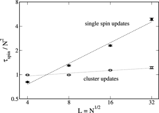
Figure 9: Scaling of the mean first-passage time for the $d=2$ Ising model using the simple high temperature representation with single spin updates ($\bullet$) and using the spin-multigraph representation with Swendsen-Wang cluster updates ($\square$). The lines are drawn as a guide to the eye.

As the weight of a spin-multigraph configuration is a product of bond weights, a cluster update scheme such as the Swendsen-Wang sw or Wolff algorithm wolff can be used to update the spin configuration. After choosing a flip operation for the spins, the only difference to the canonical cluster algorithms is the probability of adding a site to a Swendsen-Wang cluster: If $W_{ij}$ is the weight if either none or both sites are flipped and $\tilde{W}_{ij}$ the weight after a flip of one of the sites (note that this requires $W_{ij}(\sigma_{i},\sigma_{j})=W_{ij}(\sigma^{\prime}_{i},\sigma^{\prime}_{j})$ and $W_{ij}(\sigma^{\prime}_{i},\sigma_{j})=W_{ij}(\sigma_{i},\sigma^{\prime}_{j})$), the probability of adding a site to a cluster is given by

$$P_{\mathrm{connect}}=1-\min\Big{[}\frac{\tilde{W}_{ij}}{W_{ij}},1\Big{]}.$$ (50)

For the canonical ensemble simulation of the Ising model with $W(\uparrow,\uparrow,\beta)=e^{\beta}$ and $W(\uparrow,\downarrow,\beta)=1$, Eq. (50) reduces to the well known $1-e^{-\beta}$ for parallel spins as discussed before. In the spin-multigraph representation the probability to add a site to a cluster is

$$P_{\mathrm{connect}}=1-\min\Big{[}\Big{(}\frac{h_{ij}[\sigma_{i},\sigma^{\prime}_{j}]}{h_{ij}[\sigma_{i},\sigma_{j}]}\Big{)}^{\omega_{ij}},1\Big{]}.$$ (51)

Thus only sites that are connected by at least one bond of the multigraph can be added to the cluster. For the Ising model with $h_{ij}[\sigma_{i},\sigma_{j}]=\delta_{\sigma_{i},\sigma_{j}}$, the weight of a configuration $(\sigma,\omega)$ as defined in Eq. (48) is

$$W_{\beta}(\sigma,\omega)=\Delta(\sigma,\omega)\frac{\beta^{n(\omega)}}{\prod_{\langle ij\rangle}\omega_{ij}!},$$ (52)

where $\Delta(\sigma,\omega)=1$ if all bonds in the multigraph $\omega$ are satisfied and $0$ otherwise, and $P_{\mathrm{connect}}$ simplifies to $1$ if two sites are connected by one or more bonds in the multigraph and to $0$ if they are not. $O(n)$ models can be simulated by performing the spin update with respect to a mirror plane that is randomly chosen for one cluster update wolff .

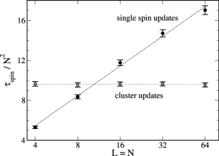
Figure 10: Scaling of the mean first-passage time to reach a low energy state for the $d=1$ XY model using single spin updates ($\bullet$) and Swendsen-Wang cluster updates ($\square$) in the spin-multigraph. Lines are drawn as a guide to the eye.

In a local update scheme, a configuration update $\sigma\rightarrow\sigma^{\prime}$ at fixed $\omega$ will be accepted with probability

$$P_{\sigma\to\sigma^{\prime}}=\min\!\Big{[}\prod_{\langle ij\rangle}\Big{(}\frac{h_{ij}[\sigma^{\prime}_{i},\sigma^{\prime}_{j}]}{h_{ij}[\sigma_{i},\sigma_{j}]}\Big{)}^{\omega_{ij}},1\Big{]}.$$ (53)

We have applied a flat-histogram sampling of this representation to the $d=2$ Ising model with periodic boundary conditions and to the $d=1$ XY model with open boundary conditions. To compare the effectiveness of the cluster updates to the single-spin flip updates, we measure the mean first-passage time $\tau_{\mathrm{spin}}$ from a random state $\sigma$ at $n=0$, which is equivalent to $\omega_{ij}=0$ for all $\langle ij\rangle$, to an ordered state. For the Ising model this state is chosen to be the ground state and for the $d=1$ model any state which is within 2.5% of the width of the spectrum to the ground state. We perform a fixed ratio of spin to multigraph updates and measure the mean first-passage time in spin updates for different ratios of spin to multigraph updates. $\tau_{\mathrm{spin}}$ converges to a fixed number with an increasing fraction of multigraph updates, and for sufficiently many multigraph updates we can assume the multigraph is equilibrated for a particular configuration. The cutoff $\Lambda$ is chosen so that the average $n$ for which the ground state is reached is much smaller than $\Lambda$.

Figure 9 shows the scaling of $\tau_{\mathrm{spin}}$ for the $d=2$ Ising model for single-spin flips in the simple representation of Eq. (42) and for Swendsen-Wang cluster updates in the spin-multigraph representation. The single-spin flip updates show a power law behavior with $z=0.85\pm 0.06$, while the cluster updates can be fitted by a logarithmic behavior or a power law with $z=0.10\pm 0.02$. Figure 10 shows the scaling of $\tau_{\mathrm{spin}}$ for the $d=1$ XY model using single spin updates and Swendsen-Wang cluster updates in the spin-multigraph representation.

IV Changing the ensemble: Optimizing the sampled histogram

An alternative to changing the dynamics from local to cluster updates for flat-histogram sampling is to optimize the simulated statistical ensemble and retain local spin-flip updates. When simulating a flat-histogram ensemble, the random walker is slowed down close to a critical point, which is reflected in the suppressed local diffusivity. To overcome this critical slowing down, we can use this information and define a new statistical ensemble $w(E)$ by feeding back the local diffusivity $D(E)$ EnsembleOptimization . After the feedback additional weight is shifted toward the critical point. The new histogram is no longer flat, but exhibits a peak at the critical energy, that is, resources in the form of local updates are shifted toward the critical point. Ultimately, this feedback procedure results in an optimal histogram $n_{w}(E)$ that is proportional to the inverse of the square root of the local diffusivity $D(E)$

$$n_{w}(E)\propto\frac{1}{\sqrt{D(E)}}.$$ (54)

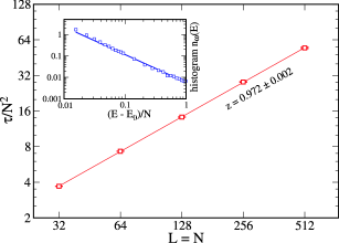
Figure 11: Scaling of the mean first-passage time of the optimized ensemble for the $d=1$ Ising model using Metropolis updates. The solid line corresponds to a power-law fit with exponent $0.972\pm 0.002$. The inset shows the optimized histogram which exhibits a power-law divergence $[(E-E_{0})/N]^{1.30}$.

For the $d=2$ Ising model it was shown in Ref. EnsembleOptimization, that the mean first-passage time scales as $\tau\propto(N\ln N)^{2}$ for the optimized ensemble and satisfies the scaling of an unbiased Markovian random walk up to logarithmic corrections. It also was found that the distribution of statistical errors in the calculated density of states $g(E)=n_{w}(E)/w(E)$ is uniformly distributed in energy, in contrast to calculations based on flat-histogram sampling.

Here we show results for the optimized ensemble of the $d=1$ Ising model for both Metropolis and $N$-fold way updates NFoldWay . For single-spin flip Metropolis updates, we find that the histogram is shifted toward the ground-state energy $E_{0}=-N$ and follows a power-law divergence, $n_{w}(E)\propto[(E-E_{0})/N]^{1.30\pm 0.01}$ (see the inset of Fig. 11). However, the mean first-passage time of the random walk in the energy interval $[-N,0]$ still exhibits a power-law slowdown with $z=0.972\pm 0.002$ as illustrated in the main panel of Fig. 11. This remaining slowdown may originate from the slow dynamics that occurs whenever two domain walls reside on neighboring bonds, and a spin flip of the intermediate spin is suggested with a probability of $1/N$. This argument suggests that changing the dynamics from simple Metropolis updates to $N$-fold way updates would strongly increase the probability of annihilating two neighboring domain walls.

We optimized the ensemble for $N$-fold way updates and found that the mean first-passage time is further reduced and scales as $\tau\propto(N\ln N)^{2}$ as shown in Fig. 12. This scaling behavior corresponds to the results for the optimized ensemble for the $d=2$ Ising model EnsembleOptimization . However, for the $d=2$ model the optimized ensembles for both Metropolis and $N$-fold way updates resulted in the same scaling behavior of the form $\tau\propto(N\ln N)^{2}$.

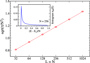
Figure 12: Scaling of the mean first-passage time of the optimized ensemble for the 1D Ising model using $N$-fold way updates (note the linear scale on the $y$-axis). The solid line corresponds to a logarithmic fit. The inset shows the optimized histogram.

V Conclusions

We have studied the performance of flat-histogram simulations of Ising and Potts models in different dimensions. For one, two, and three dimensions the simulations show critical slowing down with a critical exponent $z>0$. This behavior is analogous to the critical slowing down of canonical ensemble simulations of these models using single spin updates. Our numerical results show that $z$ decreases as a function of the dimensionality $d$ and vanishes (up to logarithmic corrections) for the infinite range Ising model.

We demonstrated that the critical slowing down of the flat-histogram simulations can be overcome by either changing the representation of the system to allow cluster updates or by changing the simulated ensemble and keeping local updates. In order to apply cluster updates to continuous spin models in connection with broad-histogram simulations, we introduced a new spin-multigraph based representation. The broad-histogram simulations which take advantage of cluster updates or an optimized statistical ensemble do not suffer from critical slowing down and show optimal scaling in comparison to an unbiased Markovian random walk.

- (1) Fugao Wang and D. P. Landau, Phys. Rev. E 64, 056101 (2001).
- (2) Fugao Wang and D. P. Landau, Phys. Rev. Lett. 86, 2050–2053 (2001).
- (3) D. P. Landau in The Monte Carlo Method in the Physical Sciences, edited by J. E. Gubernatis, AIP Conference Proceedings, 690, 134 (2003).
- (4) P. Dayal, S. Trebst, S. Wessel, D. Würtz, M. Troyer, S. Sabhapandit, and S. N. Coppersmith, Phys. Rev. Lett. 92, 097201 (2004).
- (5) S. Trebst, D. A. Huse, and M. Troyer, Phys. Rev. E 70, 046701 (2004).
- (6) W. Janke and S. Kappler, Phys. Rev. Lett. 74, 212 (1995).
- (7) C. Yamaguchi and N. Kawashima, Phys. Rev. E 65, 056710 (2002).
- (8) T. Neuhaus and J. S. Hager, J. of Stat. Phys. 113, 47 (2003).
- (9) R. H. Swendsen and J.-S. Wang, Phys. Rev. Lett. 58, 86 (1987).
- (10) U. Wolff, Phys. Rev. Lett. 62, 361 (1989).
- (11) C. M. Fortuin and P. M. Kasteleyn, Physica 57, 536 (1972).
- (12) S. Redner, A Guide to First-Passage Processes, Cambridge Universiy Press (2001).
- (13) In Ref. tt the exact density of states was found using the Mathematica program of Beale Beale ; here we used a C program and an infinite precision integer arithmetic package that also implements Beale’s approach. The latter approach allowed most of the calculation of the density of states to be spread over many processors.
- (14) P. D. Beale, Phys. Rev. Lett. 76, 78–81 (1996).
- (15) S. Reynal and H. T. Diep, cond-mat/0409529, propose another cluster approach for flat-histogram methods.
- (16) M. Troyer, S. Wessel, and F. Alet, Phys. Rev. Lett. 90, 120201 (2003).
- (17) A. W. Sandvik and J. Kurkijärvi, Phys. Rev. B 43, 5950 (1991).
- (18) A. B. Bortz, M. H. Kalos, and J. L. Lebowitz., J. Comput. Phys. 17, 10 (1975).