Information Horizons in Networks

Abstract

We investigate and quantify the interplay between topology and ability to send specific signals in complex networks. We find that in a majority of investigated real-world networks the ability to communicate is favored by the network topology on small distances, but disfavored at larger distances. We further discuss how the ability to locate specific nodes can be improved if information associated to the overall traffic in the network is available.

Not all different parts interact directly with all other parts in a complex system. Rather each element interacts directly only with a few particular elements. Distant parts of the thereby formed network can consequently communicate through sequences of local interactions. In this way all parts of the network in principle can be reached from other parts, but not all such communications are equally easy or accurate. The network is thus a description of the limited ability to send specific signals in the system rosvall . We stress the difference between specific signaling in networks and the contrary unspecific broadcasting: Where specific signaling only focuses on locating one specific node without disturbing the remaining network, the non-specific broadcasting amplifies by transfering signals to all exit links of every node along all branching paths. Specific signaling is thus constructive communication, whereas non-specific broadcasting rather is of relevance for disease spreading or computer virus propagation moreno ; newmanVirus .

One can imagine various ways of searching a specific node in a network, dependent on the available information when the search is performed adamic . In present paper we compare ways to guide the search based on locating the shortest path between a source and a target in the network. Thus we are only characterizing specific signaling, where any deviations from shortest paths mean the loss of the signal. In other words, the cost of deviating from the shortest path is assumed to be infinite, and we simply quantify the search in terms of the number of questions needed to follow the shortest path to the target.

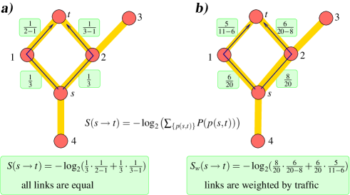
Figure 1: Information measures on network topology: a) Search Information $S(s\to t)$ measures your ability to locate node $t$ from node $s$. b) Weighted Search Information $S_{w}$ measures your ability to locate target node $t$ from the source node $s$, when you tend to follow the traffic given by the betweenness $b_{ij}$. $S(s\to t)$ is the number of yes/no questions needed to locate any of the shortest paths between node $s$ and node $t$. For each such path $P(p(s,t))\;=\;\frac{1}{k_{s}}\;\;\prod_{j}\frac{1}{k_{j}-1}$, with $j$ counting nodes on the path $p(s,t)$ until the last node before $t$. The factor $k_{j}-1$ instead of $k_{j}$ takes into account the information gained by following the path. $S_{w}(i\to j)$ is the similar quantity where we now weight each exit link from a node with its betweenness $\beta_{lk}$ freeman ; between , defined as the fraction of messages that go through node $l$ which also go through neighbor node $k$.

First let us consider the Search Information introduced in pnas . The Search Information of going from source node $s$ to target node $t$, $S(s\rightarrow t)$, is the number of bits of information one needs to go from $s$ to $t$ using the shortest paths: In the beginning, when starting at node $s$, one has to find the right exit link,$leadingto$ the second node on the shortest path to the target node $t$. We assume that each node is a simplistic autonomous system that knows which of its exit links that leads to the target. The number of questions one has to ask such an autonomous system in a source node is $\log_{2}(k_{s})$, where $k_{s}$ is the degree of the source. At the subsequent node, $j$, along the shortest path to the target the number of questions is reduced to $\log_{2}(k_{j}-1)$ since the incoming link is known. That means that the number of questions one has to ask when walking along the path from the source to the target is $S(s\rightarrow t)=-\log_{2}(\frac{1}{k_{s}}\prod_{j}\frac{1}{k_{j}-1})$. If there are more than one shortest path between $s$ and $t$, then:

$$S(s\rightarrow t)=-\log_{2}\left(\sum_{\{p(s,t)\}}\frac{1}{k_{s}}\prod_{j}\frac{1}{k_{j}-1}\right),$$ (1)

where the sum runs over the set $\{p(s,t)\}$ of degenerate shortest paths between $s$ and $t$, see Fig. 1.

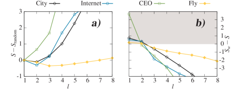
Figure 2: Analysis of real world networks. Here City is the information city network of Malmö city with roads mapped to nodes and intersections to links. The Internet refers to the hardwired networks of autonomous systems internet , the CEO to the network of cooperate executives in US ceo and Fly to the protein-protein network of Drosophilia Melanogaster giot . In a) we compare $S(l)$ with the similar search performed in a randomized version of the network. One observes that search on short distances $l\sim 2-3$ is relatively optimized in the real networks. In b) we compare $S$ with the search obtained when one uses the information associated to overall traffic in the network. We see that such global traffic information helps the search at all long distances.

In the previous work pnas we investigated $S$ for a number of networks and found that one needs more information to orient in real- than in random networks. By random networks we mean the networks randomized by the reshuffling of links in such a way as to preserve the degree sequence and keep the network connected maslov2002 . To explore the nature of these complications in real world networks we, in Fig. 2, look at the average Search Information for nodes separated by $l$ links and compare it with the corresponding quantity in a randomized counterpart. From $\Delta S(l)=\langle S(l)\rangle-\langle S_{random}(l)\rangle$ we see that essentially all the contribution to the global excess of $\Delta S=S-S_{random}$ comes from large distances $l>3$ ($S=\frac{1}{N^{2}}\sum_{s,t}S(s\to t))$. For some of the networks, as for example Internet, Yeast and Fly, the $\Delta S(l)$ is even negative at short distances, which implies that these real networks are organized to optimize the search at these short distances. Thus local specificity is favored whereas communication beyond the horizon $l=l_{search}\sim 3$ is disfavored.

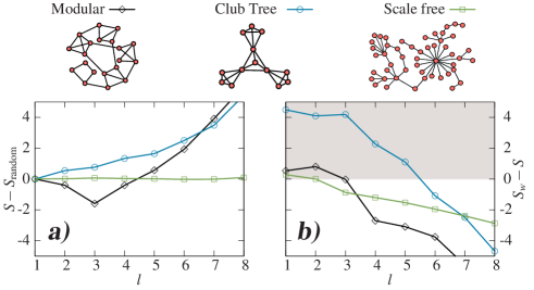
Figure 3: Analysis of model networks in terms of the quantities in Fig. 2. The simple modular network is constructed of $C$ modules with $C$ nodes in each, with $0.2C$ connections between nodes in modules and $0.2C$ connections between the modules ($C=\sqrt{N}$). The club tree is a hierarchical network with club structure at each level, a construction intended to mimic our view of social organization. We used a version with $\langle k\rangle=6$ neighbors per node and with $\approx log(N)/log(\langle k\rangle/2)$ hierarchical levels. The scale-free network is an example of networks with broad degree-distributions, here scaling as $1/k^{2.4}$. In all cases we simulate $N=5000$ node networks.

To uncover how the topology and the search information, quantified by $S$, are coupled we, in Fig. 3 investigate a number of model networks. Fig. 3(a) shows $S(l)-S_{random}(l)$ for the various model networks. We see that the search is easy at distance $l\sim 3$ in the modular network, whereas a randomly rewired network provides better search options for $l>3$. The hierarchical club network, on the other hand, clearly does worse than a random network on all scales. Here we have obtained a surprising and counterintuitive result that hierarchies are not always optimal for search. That (club)hierarchies are used in many human organizations may thus be seen as a way to regulate and thus limit the information exchange, rather than to optimize overall specific communication footnote .

The search information $S$ defined above is based on a minimal approach where one at each node knows nothing about the relative importance of the neighbors. However, in real social networks one often knows who is best connected to the rest of the system. For example in a military hierarchy, every soldier knows who their immediate superior is. This knowledge can be obtained self consistently at any node in any network by monitoring the traffic of orders past this node. In order to explore how the search can be simplified by additional knowledge we introduce a slightly different quantification of search information. That is, we explore the information needed to search if one knows the overall traffic flow. When questioning the minimal autonomous system at a node, we weight the questions according to the betweenness of the links to the node freeman ; between . Thereby we define the weighted search information

$$S_{w}(s\rightarrow t)=-\log_{2}\left(\sum_{\{p(s,t)\}}b_{s,j=1}\prod_{j\in p(s,t)}b^{\prime}_{j,j+1}\right),$$ (2)

where $j$ labels the node on the path $p(s,t)$, starting at $j=1$ for neighbor node to $s$. $b_{j,j+1}=\beta_{j,j+1}/\sum_{k}\beta_{j,k}$ is the betweenness of the link from node with label $j$ to node with label $j+1$, divided by the sum of the betweennesses of all $k$ links from $j$. $b^{\prime}_{j,j+1}$ is similarly defined except that the normalization excludes the link to the preceding node of $j$ on the shortest path between $s$ and $t$.

To understand the difference between $S$ and $S_{w}$ we consider a city (defined through the city network where each node is a road, and each link an intersection city ). By orienting yourself with the strategy behind $S$ small and large roads are weighted equally. However, $S_{w}$ captures that large roads more often take you closer to the target than small roads. For all investigated networks one in average gains by using the weighted search strategy. However, the contribution is not homogeneously distributed over distance. As one can see in Fig. 2(b) the weighted strategy is more efficient at longer distances, $l>3$. However $S_{w}>S$ for $l\leq 3$ and thus it turns out to be inefficient to follow the flow when the target is nearby. This reflects the fact that if you follow the flow you will nearly always overlook small roads in your neighborhood. In terms of navigating in a city, the $S_{w}(l)-S(l)$ difference shows that it pays off to follow the large roads until you are within a few turns from your end target. Then it naturally pays off to change strategy and disregard the main stream. The distance where $S_{w}(l)-S(l)$ becomes negative therefore defines a characteristic search horizon, $l_{local-global}$, at which one should switch from local to global search strategy.

We next study the relative advantage of local versus global search strategies for some model networks in Fig. 3(b). Like the real world networks, also the model networks have $S_{w}>S$ at small distances, and $S_{w}<S$ at large distances. In particular, the club tree (hierarchy) does extremely bad at short distances because there is a strong bias to go along the main flow, and one thus needs a lot of effort to locate peripheral neighbors. For a random scale-free network, on the other hand, the overall traffic very fast guides you to the center, and therefore $S_{w}$ is a good search strategy at nearly all distances. The scale-free network represents topologies with very broad degree distributions and in these one nearly always benefit by following the flow adamic .

In between these two networks is the modular network, where the global flow confuses local search ($S(l<3)<S_{w}(l<3)$), but helps traffic to other modules and thus to the more distant targets. Returning to the real world networks in Fig. 2(b) their $l_{local-global}\sim 2$ horizon for traffic guided search may be seen as a combination of a short $l_{local-global}\sim 1$ horizon associated to their broad degree distribution (scale free in Fig. 3(b)), and a larger $l_{local-global}$ horizon associated to modular or hierarchical features.

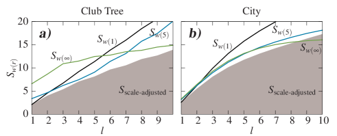
Figure 4: Investigations of search strategies in a model network a) and information city network of Malmö b). The figures illustrate 3 simple search strategies, and one optimized (shaded). $S_{w(r)}(l)$ denotes the search information based only on traffic between nodes separated by not more than $r$ steps in the network. We see that nodes on short distance are best found by using local search strategy ($S_{w(r=1)}=S$, whereas search to distant nodes are best performed by using information from global traffic. However, nodes at intermediate distances are best found by using traffic between nodes at intermediate distances. To optimize search we also show a different search strategy $S_{\mathrm{scale-adjusted}}$, where one at each step $j$ along the path to the target adjust the traffic horizon to the remaining distance to the target. We furthermore restrict the traffic bias to the subset of traffic that are targeted to the node $j$ one is currently at (see Fig. 5).

One may ask whether the two search strategies can be combined, such that one uses local information for local search, and global traffic information for long distance search. In terms of traffic in a city the picture is that there are multiple types of traffic, from pedestrian to short distance targets, bicycles to intermediate distance targets, to cars for the distant targets. In accordance to this picture we introduce the limited betweenness measures $b_{ij}(r)$ for the links $j$ around a node $i$, defined by traffic between all pairs of nodes that only moves at maximum a distance $r$ between the source and the target. Given this set of $r$ dependent traffic weights, we in analogy with Eq. 2, define a set of search measures $S_{w(r)}(l)$. For $r=1$, $S_{w(1)}(s\rightarrow t)=S(s\rightarrow t)$, whereas $S_{w(r=\infty)}(s\rightarrow t)=S_{w}(s\rightarrow t)$ and thus $S_{w(r)}$ naturally interpolates between the non-weighted and the traffic-weighted search approaches. In Fig. 4(a) we examine $S_{w(r)}(l)$ for the club-hierarchy network from Fig. 3. In accordance with Fig. 3(a) we again see that the longer distances indeed are best searched by using long distance traffic. In addition we see that intermediate distances $l=3-7$ are best searched by using a search weighted by traffic traveling intermediate distances $r\sim 5$, as quantified by $S_{w(5)}(l)$.

Fig. 4(b) shows the optimal search strategy in a real network, here the information city network of Malmö city . Again the search efficiency is improved by adjusting the traffic horizon to the search distance. In fact the search can be further optimized by, at each step, adjusting the traffic horizon $r$ to the remaining distance to the target. In the language of city networks, when searching a distant road, one first uses information from car traffic, but as distance to target becomes smaller than say 5 intersections, one instead uses bicycle- and then subsequently pedestrian traffic. This overall feature of optimizing search works best when one weights the exit link from each node $j$ by the fraction of overall traffic target explicitly to $j$. Thus, the optimal search indicated by the shaded area in Fig. 4 corresponds to a search strategy, where one at each step $j$ from $s$ to $t$ bias the search according to the subpart of the traffic that is targeted at $j$, and which has a source at distance that are not further away than the target $t$ (see Fig. 5). The difference to the normal betweenness is that the target betweenness effectively partitions the network around each node $j$, such that each exit link is weighted by the fraction of the network that it leads to. This therefore provides a more efficient guess on the direction to the rest of the network from $j$ than the normal betweenness.

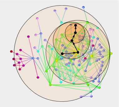
Figure 5: Illustration of optimal search strategy on an information city network of Gamla stan, Stockholm city : At each step the contribution to the traffic bias is limited by sequentially decreasing horizons (circles). The radius of each horizon reflects the node distance to the target. In case of the large city, each horizon corresponds to the type of transportation one should consider: Within the big circle one looks for cars and within the smallest circle for pedestrians. The path is indicated in black.

Obviously the optimal search strategy can only be used if one has access to this distant-dependent traffic information. However, as in a city, such information can for example be quite well estimated in social networks. Consider Milgram’s famous result of a mail locating a target person in a chain of typically six acquaintances between two persons in USA milgram . The nontrivial result of Milgram’s experiment is not that the distance between two persons is just six, since the dimension in social networks are high kochen , but the fact that short paths were found in the experiment. In terms of our optimal search strategy, Milgram’s experiment is interpreted the following way: Every participant that receives a mail aimed to a distant target person, gives this in his turn to a friend, with a chance weighted to how often this friend travels on distances up to the scale of the target distance. With such a search strategy, that at each point along the path is adjusted to the horizon to the target, the mail will find a short path to the target person with high probability (low information cost). We speculate that humans inherently tend to use such a scale-free search strategy, and by this facilitate robust communication on all scales ranging from a single remote village to the whole planet. The information gain by doing so in the city Malmö is illustrated by the difference between the black curve and the shaded area in Fig. 4(b).

In the present work we have quantified the information cost associated to transmission of specific signals across a complex network. By comparing real- and random networks, we have shown that many real-world networks tend to have optimized searchability at rather short distance $l\sim 3$. The cost of this optimization is that beyond this horizon one must use more intelligent methods to facilitate searchability. In the spirit of communication we have investigated methods based on global traffic observed at local level and interpreted them in real-world examples.

In many networks, in particular social or traffic networks, the search strategy can be adjusted according to average traffic flow. The distance at which global traffic becomes superior to unbiased search defines a horizon associated to the largest scale of modules in a network. In general, any network we have investigated are best searched by using the “scale invariant” strategy, where directions are selected according to the average traffic to nodes at distances similar to that of the searched target node.

References

- (1) M. Rosvall and K. Sneppen, Phys. Rev. Lett. 91, 178701 (2003).
- (2) Y. Moreno and A.Vazquez. Eur. Phys. J. B. 31 265 (2003).
- (3) J. Balthrop, S. Forrest, M. E. J. Newman, and M. M. Williamson, Science 304, 527 (2004).
- (4) L. Adamic, B. Huberman, R. Lukose and A. Puniyani, Phys. Rev. E 64, 46135 (2001).
- (5) L. C. Freeman, Sociometry 40, 35 (1977).
- (6) M. E. J. Newman. Phys. Rev. E 64, 016132 (2001).
- (7) K. Sneppen, A. Trusina and M. Rosvall, cond-mat/0407055 (2004).
- (8) M. Rosvall, A. Trusina and K. Sneppen, cond-mat/0407054 (2004).
- (9) G. F. Davis and H.R. Greve, American Journal of Sociology 103, 1 (1997).
- (10) L. Giot et al., Science 302, 1727 (2003).
- (11) S. Maslov and K. Sneppen, Science 296, 910 (2002).
- (12) S. Milgram Psychol. Today 1, 61 (1967).
- (13) M. Kochen, Ed., “The Small World” (Ablex, Norwood, 1989).
- (14) Website maintained by the NLANR Measurement and Network Analysis Group at http://moat.nlanr.net/
- (15) The hierarchical search algorithms are however effective, but only in the specific case of perfect tree-like hierarchy searched from the top. In that case the measured from the top is which is a smaller search information than for any other organization of a network consisting of nodes.
- (16) We acknowledges the support of Swedish Research Council through Grants No. 621 2003 6290 and 629 2002 6258.