Dielectric resonances in disordered media

Abstract

Binary disordered systems are usually obtained by mixing two ingredients in variable proportions: conductor and insulator, or conductor and super-conductor. They present very specific properties, in particular the second-order percolation phase transition, with its fractal geometry and the multi-fractal properties of the current moments. These systems are naturally modeled by regular bi-dimensional or tri-dimensional lattices, on which sites or bonds are chosen randomly with given probabilities. The two significant parameters are the ratio $h=\sigma_{1}/\sigma_{0}$ of the complex conductances, $\sigma_{0}$ and $\sigma_{1}$, of the two components, and their relative abundances $p$ (or, respectively, $1-p$). In this article, we calculate the impedance of the composite by two independent methods: the so-called spectral method, which diagonalises Kirchhoff’s Laws via a Green function formalism, and the Exact Numerical Renormalization method (ENR). These methods are applied to mixtures of resistors and capacitors (R-C systems), simulating e.g. ionic conductor-insulator systems, and to composites consituted of resistive inductances and capacitors (LR-C systems), representing metal inclusions in a dielectric bulk. The frequency dependent impedances of the latter composites present very intricate structures in the vicinity of the percolation threshold. In this paper, we analyse the LR-C behavior of compounds formed by the inclusion of small conducting clusters (“$n$-legged animals”) in a dielectric medium. We investigate in particular their absorption spectra who present a pattern of sharp lines at very specific frequencies of the incident electromagnetic field, the goal being to identify the signature of each animal. This enables us to make suggestions of how to build compounds with specific absorption or transmission properties in a given frequency domain.

1 Introduction

Composite materials, obtained for instance by mixing powders, are increasingly used in modern mechanical, electrical and optical devices. Their extraordinary properties often meet the very compelling standards needed for high technology materials, e.g. high temperature resistance, low density, and low thermal or electrical conductivity. Their manufacturing is however extremely delicate and requires a good comprehension of the microscopic and macroscopic properties of the different constituents. The goal of this paper is to provide a better theoretical understanding of various electrical properties of these materials, especially in the high frequency domain.

Composite systems are commonly thought of as random networks where each bond represents, via a complex impedance, a grain or a grain boundary. The various constituents of the composite material are then randomly distributed over the network, and elements of the same type connected to each other form “clusters”, or “animals” in the terminology of Pierre-Gilles de Gennes. The interfaces between clusters are usually the physically most interesting regions Debi ; Gilbert . Therefore, in binary composites, the percolation of one component through the other plays an essential role: the properties of the material change dramatically for small variations of the chemical composition in the vicinity of the percolation threshold, giving rise to a second-order phase transition which allows the physicist to put a large number of disordered systems in the same universality class.

These heterogeneous media occur mainly as bulk material occupying a 3D volume, or as thin, almost 2 dimensional, layers upon a substrate. In both cases, the electrical properties, i.e. the frequency-dependent network impedance, can be obtained as a direct solution of Kirchhoff’s Laws for each network node. As this involves the diagonalisation of large matrices, this method becomes very expensive in CPU time as soon as realistic systems are to be modelled. On the other hand, a crude mean-field approximation, although generally qualitatively correct, is not sophisticated enough to reproduce experimental results quantitatively.

Alternative approaches are provided by spectral methods, based on the theory of random walks (see the excellent article by W.H. McCrea and F.J. Whipple McCrea , and the book of F. Spitzer Spitz ). These approaches have been extended to percolation phenomena Clerc2 ; Luck and work particularly well in two dimensions. For a random 2D network, the electrical and optical properties are described by its analytically obtainable conductance poles (resonances) and their residues (weights). This approach can also be extended to binary disordered media in 3D, as shown by two of the authors in a previous paper, although the possibility of an analytic treatment is lost Laurent .

One goal of the present paper is to study the elementary clusters, or “animals”, which take part in percolation until the threshold is reached and the cluster becomes infinite. A detailed description of an algorithm generating all animals for a given number of bonds (“legs”), and the complete “zoo” of up to 4-legged animals will be given in the appendix. A composite’s response to a frequency-dependent electromagnetic signal is a highly characteristic spectrum which can be viewed as the signature of conducting clusters (animals) embedded in a dielectric medium. In the dilute limit, where the influence of one animal on its neighbors is negligible, one measures the almost unperturbed spectral fingerprint of the individual animals. In this case, a theoretical study of the spectra of a limited number of small, elementary animals provides a good starting point for the interpretation of the response of the composite as a whole. Still provided the concentration of metallic clusters is low, one may even be confident to gain some insight into the microscopic structure of the material itself.

Our aim is to compare these results to those of the renormalization algorithm described below. The latter remains very efficient even if the animals become large, or if elementary animals are arranged as regular arrays over the whole lattice, cases for which the exact spectral calculations become very cumbersome. The algorithm implemented for performing these simulations is called Exact Numerical Renormalization (ENR) and was initially proposed in Ref. Vinograd ; Sarych ; Tort . The basic idea is to eliminate network nodes successively, and to connect all neighbors of the eliminated site by bonds with renormalized impedances. The method is essentially applicable to any connected network, regardless of dimensionality and connectivity. In the following, however, we will restrict our considerations to the hypercubic lattices in two and three dimensions. We will evaluate the impedance versus frequency curves of metallic animals, constituted of bonds, or legs, to which a complex conductivity is attributed, on square (2D) and simple cubic (3D) dielectric lattices.

The notations of this paper are those of Ref. Clerc2 ; Clerc1 ; we recall them shortly. The bond occupation is obtained according to the following binary law: conductance $\sigma_{0}$ and concentration $p$ for one kind of bond (representing the animal’s legs), $\sigma_{1}$ and $1-p$ for the rest of the lattice (voids). The dimensionless complex ratio $h=\sigma_{1}/\sigma_{0}$ of the two conductances and the relative abundance $p$ are the essential parameters of the model. For convenience, $h$ may be replaced by the equivalent complex variable

$$\lambda=\frac{1}{1-h}=\frac{\sigma_{0}}{\sigma_{0}-\sigma_{1}}$$ (1)

For the 2D case, the square lattice is self-dual, and quantities such as the percolation threshold, or spectral properties of some animals, can be easily deduced from this particularity. In 3D, the self-duality property is lost. In section 2, we recall the analytic method and the numerical algorithm. In section 3, we examine the spectral properties of elementary animals and the particularities which arise if such metallic animals are disposed as regular super-arrays on a dielectric lattice; the real and imaginary parts of the impedance are presented and discussed for a large panel of such animals. In section 4, we are concerned by binary random lattices and the corresponding Nyquist diagrams. The recursive algorithm used for the creation of all $n$-animals (with $n$ being the number of legs), and the symmetry properties of animals with $n\leq 9$ are discussed in the appendix. We conclude the paper by proposing some applications of binary random networks.

2 Model and algorithm

We consider a binary composite constituted of a random distribution of electrical bonds and voids on a hypercubic lattice. The total conductance $Y$ of the sample (or, alternatively, its impedance $Z={1}/{Y}$), is obtained by the fulfillment of Kirchhoff’s Current Law at each network node $x$:

$$\sum_{y(x)}\sigma_{x,y}(V_{x}-V_{y})=\sum_{y(x)}I_{x,y}=I_{x}$$ (2)

with $V_{x}$ corresponding to the potential at node $x$, $I_{x}$ the current arriving on the node $x$, and $I_{x,y}$ the current from $y$ to $x$ along the link of conductance $\sigma_{x,y}$. If a total current $I$ flows through the sample between the two electrodes, of which one is at potential $V_{1}$ and the other grounded ($V=0$), the conductance of the network reads $Y=I/V_{1}$. Only the finite section ${\cal L}$ of a square (2D) or cubic lattice (3D) in-between the two electrodes is considered. In three dimensions, this piece is characterized by

$${\cal L}=\{1\dots N_{x}\}\times\{1\dots N_{y}\}\times\{1\dots(N_{z}-1)\}\,.$$

The plans $z=0$, and $z=N_{z}$ (respectively $y=0$, and $y=N_{y}$ in the 2D case) are taken as electrodes. Each link of this binary network is assumed to have either conductance $\sigma_{0}$ with probability $p$, or conductance $\sigma_{1}$ with probability $q=1-p$. In order to reduce finite-size effects, periodic boundary conditions are imposed in all directions parallel to the electrodes, i.e. in the $x$ ($x$ and $y$) direction in 2D (3D, respectively).

A convenient alternative to a direct solution of Kirchhoff’s Laws is the spectral method in which the spectrum results from a solution of a generalized eigenvalue problem. This spectrum presents a rich set of resonances, characteristic of the bond distribution and the underlying lattice structure. This approach, proposed by Straley Stra and Bergman Berg , yields the conductivities, corresponding to different values of $h=\sigma_{1}/\sigma_{0}$, by means of the frequencies and weights of the conductance poles. Instead of the bare $h$ itself, one may of course use the handier parameter $\lambda={1}/(1-h)$ defined in eq. (1) which confines the poles to the interval $[0,1]$.

It has been adapted to 2D finite networks in Ref. Luck and enhanced to 3D in Ref. Laurent . However, as larger networks are to be treated, the method becomes very time-consuming, since it involves the numerical diagonalisation of large matrices. In the following, we will therefore tackle the problem with another algorithm which is inspired from the renormalization procedure Vinograd ; Sarych ; Tort .

In this method, known as Exact Numerical Renormalisation (ENR), the network sites are eliminated one by one. At each step, the former neighbors of the eliminated site are connected by possibly new bonds whose impedances are chosen such that the global impedance of the system remains invariant. Namely, if $x$ is the site to be eliminated, the conductivity $\sigma_{i,j}$ between all sites $i$ and $j$ of the neighborhood of $x$ will be reassigned to $\sigma_{i,j}^{*}$. It is easy to verify that $\sigma_{i,j}^{*}$ is given by

$$\sigma_{i,j}^{*}=\sigma_{i,j}+\frac{\sigma_{i,x}\sigma_{x,j}}{\sum_{j}{\sigma_{x,j}}}\,.$$ (3)

where the summation is over all neighbors of site $x$ Tort . Note that $\sigma_{i,j}=0$ if sites $i$ and $j$ are not connected before the elimination of $x$. The renormalization procedure is numerically exact. The ENR procedure stops when the two electrodes are linked by only one bond which then carries the total conductivity of the initial lattice. Details of calculation are given in Ref. Tort . The ENR method is particularly well adapted to a sparse medium, and can be applied to any linear network including systems with more than two components. For instance in a conductor-insulator system near the percolation threshold, each site $x$ of the infinite cluster has an average number of neighbors smaller than the connectivity of the system, and a great number of sites can be suppressed without the introduction of additional links between remaining sites. But even for the problems considered in this paper, where all bonds of the lattice must be taken into account and the renormalization has to be performed for all frequencies, the ENR algorithm is considerably faster than the spectral method developed in Ref. Luck ; Laurent . The main restriction of the ENR method is that the nature of the components has to be determined by defining a relation $h(\omega)$ or $\lambda(\omega)$ before the computation, e.g. $h(\omega)={\rm j}C\omega(R+{\rm j}L\omega)$ for the LR-C model considered in the following.

This paper is devoted to the study of:

1. Small clusters (“animals”) of a few connected conducting bonds (of inductance L and resistance R) in an insulating environment (of capacity C) Clerc2 , the aim being to detect the signature of elementary clusters in the spectral response of a conductor–insulator mixture.

2. Percolation through a binary Resistive-Capacitive lattice. For these systems, one has to sample over a large number of random networks in order to gain some information which is intrinsic to the chemical composition $p$. For disordered systems, one specific random network is not interesting, and all quantities have to be averaged over a sufficiently large number of systems of the same degree of disorder. For obvious symmetry considerations, the interchange of $p$ and $q$ corresponds to replacing $h$ by ${1}/{h}$, or $\lambda$ by $1-\lambda$. This symmetry relation allows us to confine the range of investigation of such models to $p\leq\frac{1}{2}$. Moreover, one can immediately conclude that any averaged quantity computed for $p=\frac{1}{2}$ will be symmetrical around the value $\lambda=\frac{1}{2}$. This implies, for instance, that the average conductance of the network obeys

   $$Y(p,\sigma_{0},\sigma_{1})=\sigma_{0}\tilde{Y}(p,\lambda)=\sigma_{1}\tilde{Y}(1-p,1-\lambda)\,.$$ (4)

The spectral algorithm yields the positions and cross-sections of all resonances and for any cluster (provided the cluster is not too large and the numerical calculation remains feasible Laurent ), and a fortiori for small $n$-animals ($n\leq 10$). In 2D, moreover, all quantities may — at least in principle – be evaluated analytically on an infinite lattice Clerc2 .

The ENR algorithm, on the other hand, is particularly well adapted to large clusters (percolation), and to the study of the coupling between a few animals as a function of their mutual distances. Instead of the resonance positions (eigenvalues) and the corresponding weights (which are connected to the eigenvectors), this algorithm yields readily the total frequency-dependent impedance of the whole system with the desired degree of accuracy.

3 Spectral properties of animals

In this paragraph, small metallic clusters are investigated. These “animals” are constituted of $n$ conducting bonds (“legs” of self-inductance $L$ and resistivity $R$), and “live” on an insulating lattice of capacitors $C$ Clerc2 . For the 2D case, an exhaustive list of all up to 4-legged animals living on a square lattice, together with their geometries and abundances, is given in the Fig. 1.

For animals living on a finite 3D network, the spectra show pole densities and average resonance positions which scale as the inverse of the linear size of the sample, thus corresponding to the ratio surface over volume for a cubic sample Laurent . This allows one to extrapolate the finite size results to an infinite lattice. Alternatively, the resonance values and the pole densities of a single animal on an infinite network can be evaluated exactly by the method described in Clerc2 . The positions of the resonances are then the eigenvalues of a matrix $M_{x,y}$ obtained from the values of the Green function of the laplacian operator on the infinite lattice

$$M_{x,y}=\sum_{z\in C(y)}{(G_{x,y}-G_{x,z})}\,.$$ (5)

where $x$, $y$ and $z$ belong to the conducting cluster and the index of summation, $z$, runs over the neighborhood of $y$, $C(y)$. In general, this is a $n_{s}\times n_{s}$ non-symmetrical matrix, where $n_{s}$ is the number of sites of the animal under consideration.

Figure 1: All topologically different animals (species) with one leg (one species), two legs (two species), three legs (five species), and four legs (16 species). The percentages indicate how many animals belong to a given species in a zoo.

Table 1: Exact resonance position $\lambda$ and corresponding residues for animals consisting of one, two and three bonds. Analytical results are compared to ENR results for a single LR animal in the center of a $24\times 24$ square lattice. The animals’ labels are those of Fig. 1.

animal	$\lambda$ exact	$\lambda$ ENR	residue	$Re(Z)$
1	0.5	0.5011248	4.	2.30485
2a	0.36338	0.367	8.6455	4.95521
	0.63662		0.000
2b	0.318310	0.316	2.304	1.471
	0.681690	0.6784	2.304	1.09
3a	0.28216	0.29219	14.633	9.155
	0.54648		0.000
	0.67136	0.67158	0.16406	0.1175
3b	0.24970592	0.251	6.959	4.202
	0.54315776	0.5424	2.239	1.454
	0.70713638	0.7061	0.679	0.4564
3c	0.16581640	0.167	2.686	1.8034
	0.6366200		0.000
	0.69756359	0.698	2.979	1.956
3d	0.22926367	0.243	2.718	3.693
	0.55349146		0.000
	0.55349146	0.7575	2.718	3.66
3e	0.30243640		0.000
	0.3633800	0.367	8.645	5.48
	0.8341836		0.000

It is straightforward to obtain an animal’s set of resonances (see e.g. Table 1 for all animals up to 3 legs shown in Fig. 1). The cross section (i.e. the residue) $\gamma_{a}$ of a resonance $\lambda_{a}$ can be obtained analytically. For each animal, one finds a resonance at $\lambda=0$ which has no physical meaning and carries $0$ weight Laurent .

This spectral method developed for the 2D case can be readily extended to 3D systems, but the helpful duality property gets lost in 3D.

Table 2: Resonance position and corresponding residues for some one- or two-legged animals located at various positions in a $8\times 8\times 8$ cubic lattice. Due to the boundary conditions, only the current direction ($z$) is relevant. $i_{n}$ labels a 1-animal consisting of a single bond between plans $z=n$ and $n+1$. $I_{n}$ represents a 2-animal consisting of two adjacent bonds along the same direction, between plans $z=n$ and $n+2$.

animal	pole position	residue $10^{-2}$ unit
$i_{0}$, $i_{7}$	0.789308423	4.17081055
$i_{1}$, $i_{6}$	0.674277363	7.54795650
$i_{2}$, $i_{5}$	0.668037619	7.76440136
$i_{3}$, $i_{4}$	0.667363895	7.78801367
$I_{0}$, $I_{6}$	0.570490690	0.77324464
	0.893095096	3.61773483
$I_{1}$, $I_{5}$	0.544761964	0.00397830
	0.797553018	7.93113971
$I_{2}$, $I_{4}$	0.543267933	0.00004814
	0.792133581	8.20040186
$I_{3}$	0.543157473	0
	0.791570318	8.22848890

Table 3: Similar results as in table 1 for a right-angle animal with the vertex on row $n+1$.

animal	pole position	residue $10^{-2}$ unit
$\Gamma_{0}$	0.566366254	4.05530700
	0.903637749	1.10140027
$\Gamma_{1}$	0.534390544	6.66404562
	0.808411116	1.89039118
$\Gamma_{2}$	0.531898275	6.86342706
	0.803701317	1.91149019
$\Gamma_{3}$	0.531617073	6.88538519
	0.803195822	1.91366884
$\Gamma_{4}$	0.531730016	6.88512684
	0.803195852	1.91287160
$\Gamma_{5}$	0.532860589	6.86124029
	0.803701327	1.90472208
$\Gamma_{6}$	0.546552694	6.64049976
	0.808420249	1.80603241

The resonance positions given for a finite size realization of the 3D case are presented in Table 2 and Table 3. They show the sensitivity of the spectra to the animals’ position with respect to the electrodes, and differ considerably from the 2D results listed in Table 1.

In what follows, we restrict our analysis to the 2D case but a generalization to 3D is immediate.

Figure 2: Representation of a square lattice in 2D, of size $N_{x}=N_{y}=10$. The two electrodes at $y=0$ and $y=N_{y}=10$ are, respectively, at potential $V_{1}$ (assumed $>0$) and $V_{0}=0$. Periodic boundary conditions are assumed in the $x$ direction. Twelve animals are shown for example.

Applying the formalism proposed by Clerc et al. Clerc2 , to the 2-legged animals 2a and 2b of Fig. 1, we obtain

$$M=\frac{1}{4}\left(\begin{array}[]{c c c}1&\,-(2+4g)&\,4g+1\\ -1&2&-1\\ 4g+1&\,-(2+4g)&\,1\end{array}\right)\,.$$

The value of $g$ depends on the relative orientation of the two bonds and may be obtained analytically in 2D: $g=G_{2}=\frac{2}{\pi}-1$ for two bonds in a line, and $g=G_{1,1}=-\frac{1}{\pi}$ for two orthogonal bonds. One obtains $\lambda_{1}=-g$ and $\lambda_{2}=g+1$ as eigenvalues of $M$ leading to resonances at $h_{1}=\frac{1+g}{g}$ and $h_{2}=\frac{g}{1+g}$. For self-dual animals in 2D, duality implies that the solutions occurs as pairs verifying the relations $\lambda_{1}+\lambda_{2}=1$ or $h_{1}h_{2}=1$. For two adjacent links with the same orientation, we have $g=G_{2}=-0.36338$, and the two resonances occur respectively at $\lambda_{1}=0.36338$ and $\lambda_{2}=0.63662$. For two orthogonal links, we have $g=G_{1,1}=-0.31831$, and the resonances are $\lambda_{1}=0.31831$ and $\lambda_{2}=0.68169$ (see Table 1). In both cases, these values are well confirmed by the ENR results (except that, for obvious reasons, the zero weight resonance of animal 2a cannot be detected by ENR).

For all up to 3-legged animals represented in Fig. 1, the exact and numerical eigenfrequencies, and the corresponding exact residues along with $Re(Z)_{\rm max}$ are listed in Tab. 1. The spectrum is deduced from the numerically obtained real part of the impedance versus $\omega$ or $\lambda$; within the ENR algorithm the residue of each pole is closely related to the maximum value of the real part of the impedance, $Re(Z)_{\rm max}$ Clerc2 ; Luck . For a 2D $N\times N$ lattice with $L=C=1$ and resistance $R$ varying between $1\cdot 10^{-3}$ and $2\cdot 10^{-1}$, we find:

$$Re(Z)_{\rm max}\approx\frac{\gamma_{a}}{RN^{2}}$$ (6)

For an animal in the center of a sufficiently large lattice (e.g. $N_{x}=N_{y}=24$) finite size effects – resulting in a small shift of the resonance positions – may be safely ignored. Its spectrum may be calculated for pulsations $\omega$ such that $\lambda(\omega)$ runs over the complete interval $[0,1]$.

It is numerically impossible to find resonances of zero cross-section. Therefore, animals of the same species, which necessarily have the same eigenvalues $\lambda$ — as e.g. in Fig. 2 the animals $1$ and $5$, $6$ and $7$, $4$ and $11$, and $8$ and $12$ — may be oriented differently with respect to the electrodes in order to identify, if possible, the positions of the resonances of zero weight. According to this analysis, the animal $1$ of Fig. 2, whose three sites are on the same potential, is not crossed by any current: consequently, the three resonances have zero weight and do not contribute to the conduction. The poles corresponding to diagram $7$ of Fig. 2 — a “T” with the two bonds of its horizontal bar perpendicular to the electrodes — are two times stronger than those of diagram $6$ — the same “T” but turned by $90^{\circ}$ such that only one bond is perpendicular to the electrodes. The same holds true, respectively, for the diagrams $8$ and $12$, and also for $4$ and $11$. The diagrams $2$, $3$ and $11$ present strictly the same response to an incident a.c. wave: obviously, the bonds parallel to the electrodes do not participate to the resonance phenomena at all.

For large clusters, or when several clusters are present on the surface, it is very lengthy to obtain the exact spectral responses since inter-cluster interactions must be taken into account. Under these conditions, the ENR algorithm reveals its efficiency. We only present the calculations for the 2D case. In 3D, the physical ideas are essentially the same, but the calculus becomes very cumbersome.

Figure 3: Real part $Re(Z)$ of the impedances versus $\lambda$ for various animals living on a $12\times 12$ square lattice. (a) The continuous peak at $\lambda=0.5$ is the signature of the simplest 1-animal — a single inductance — in $y$-direction. The dashed peak on its right, at $\lambda\simeq 0.63$, is obtained with two parallel coils on successive lines (animal no. 3 in Fig. 2), and the dotted-dashed peak on the left, at $\lambda\simeq 0.37$, has its origin in two adjacent inductances on the same line (animal no. 5 in Fig. 2). (b) The dashed peak on the right was obtained by two parallel coils in $y$-direction, separated by an empty line. The dot-dashed peak on the left corresponds to two coils on the same horizontal line, separated by a capacitive link. Comparison with the dashed and dot-dashed curves in Fig. 3a shows that the coupling between the coils decreases and the resonances occur closer to the value $\lambda\simeq 0.50$ (characteristic for a single coil). (c) Spectra given by various staircase-shaped animals: the continuous line, with the two peaks closest to the center, at $\lambda=0.32$ and $\lambda=0.68$, origins from two coils forming a right-angle (animal no. 9 in Fig. 2). The dashed line, showing peaks at $\lambda\simeq 0.22$ and $\lambda\simeq 0.78$, corresponds to animals no. 8 and 12 in Fig. 2. The dot-dashed line with the outermost peaks, at $\lambda\simeq 0.16$ and $\lambda\simeq 0.84$ corresponds to a four-step staircase animal. The separation in $\lambda$ between an animal’s two spectral peaks thus increases with the animal’s size. (d) Comparison of two disordered system with the same densities of coils: the full line corresponds to 36 two-bond right angles, with vertex sites chosen at random. The dashed line corresponds to 72 randomly chosen bonds, 36 of which are horizontal and the other 36 vertical.

Fig. 3, where the weights of the resonances are represented as a function of the parameter $\lambda$, shows the coupling between resistive coils placed in different locations of the capacitive lattice. In the spectra represented on Fig. 3a, each inductance ($L$,$R$) occupies a link in the $y$-direction (perpendicular to the electrodes) and it is not connected to any electrode. The central peak corresponds to two well separated coils: it occurs at $\lambda=0.5$, i.e. the resonance frequency of a single coil, but carries twice the weight. The left peak in the figure corresponds to two horizontal inductances in series, whereas the right peak corresponds to two parallel inductances separated by one lattice spacing in the $x$-direction (i.e. by capacities on either side). From duality, we know that the resonances are the same in the two cases but each time, only one peak contributes to the spectrum, while the other resonance has zero cross section. These results can be understood qualitatively in terms of, respectively, two inductances in series (inductance $\simeq 2L$, with resonance pulsation $\omega_{a}\simeq\omega_{0}/\sqrt{2}$), and two inductances in parallel (inductance $\simeq{L}/{2}$, with resonance pulsation $\omega_{b}\simeq{\omega_{0}}\cdot{\sqrt{2}}$), where $\omega_{0}=1/\sqrt{LC}$ is the resonance pulsation of a single $LC$ circuit. This simple picture yields $\lambda_{a}=0.3692$ and $\lambda_{b}=0.6410$, and almost fulfills the exact duality relation $\lambda_{a}+\lambda_{b}=1$. Note also that the maxima of the left and right peaks are approximately the same, both being very close in height to the central peak (which carries the intensity of two well separated coils): despite the coupling, the amplitudes are almost additive.

Fig. 3b illustrates that the coupling between the bonds decreases very quickly with the distance between the coils. The spectra were obtained with similar coil-capacity configurations as the outer peaks of Fig. 3a, but each time the separation between the coils was increased by interposing a capacity (empty link), shifting the peaks closer to the central value of $\lambda=0.5$, characteristic for independent coils.

Fig. 3c represents the spectra of three different staircase animals. The solid line corresponds to the spectrum of a single right angle – see animal 2b on Fig. 1; for comparison, its amplitude has been multiplied by a factor of eight. The dashed line shows the resonances of an animal corresponding to number 3d on Fig. 1 (the amplitudes are multiplied by a factor of four). Finally, the dotted-dashed line represents the response of a four-step staircase. Clearly, the relevant eigenvalues, i.e. those with non-vanishing cross sections, drift further and further apart as the size of the animal increases, while the corresponding cross-sections are roughly proportional to the number of links in the $y$-direction. Besides the main resonances visible in the figure, the animals — especially the larger ones — may contain eigenvalues of zero or almost zero weight. Note that all staircase animals are self-dual (if contained in an infinite lattice); hence the eigenvalues occur in pairs satisfying $\lambda_{1}+\lambda_{2}=1$, which provides a good check for the numerical results and yields spectra symmetric about $\lambda=0.5$.

However, if such right-angle 2-animals are randomly spread on the lattice the resulting impedance is quite different from an individual animal’s: the full line in Fig. 3d corresponds to $36$ right-angle animals distributed at random on a $12\times 12$ network (averaged over one hundred realizations) and only the peak near $\lambda\simeq 0.7$ can be identified as a signature of the right-angle structure. With the same conditions, but with $36$ horizontal bonds and $36$ vertical bonds chosen at random, the result is given by the dashed line curve of Fig. 3d.

We conclude that only in the very “dilute” limit ($p\ll 1$), the spectral features may be assigned to elementary animals, such as isolated links or pairs of links. If an animal is predominant in a network, it is easy to predict the conductivity ratio $h$, and the frequency which leads to the optimal conductivity: in practical applications, a pattern could be chosen in order to obtain a selective absorption or reflectivity for a given frequency band. This property might have some interesting practical implications which could result in the engineering of devices whose impedances might almost be chosen à la carte. As soon as the density of animals in the lattice increases, and the animals’ legs occupy in the order of $5\%$ of the lattice bonds or more, the coupling between patterns increases and with it the difficulty to assign the observed spectrum to a specific animal.

We want to draw the reader’s attention to the spectra that emerge if the coils are not randomly distributed but regularly arranged on the lattice, thus forming a regular super-structure of the dielectric lattice.

Figure 4: (a) Real part of the impedance $Re(Z)$ versus $\lambda$ for a $12\times 12$ lattice wholly occupied by capacities, except for an array of $36$ regularly distributed horizontal coils, linking sites $(x,y)$ and $(x,y+1)$ with $x$ and $y$ even. $Re(Z)$ presents a “colossal” resonance for $\lambda\simeq 0.628$. (b) Same curves for an array where each horizontal coil originates at a node $(x,y)$ with both coordinates $x$ and $y$ multiples of 3 (solid line) and 4 (dotted line). Figure (c) and (d) correspond, respectively, to Figure (a) and (b), with right-angle animals replacing the horizontal coils. The two peaks in Figure (c) occur at the same $\lambda$ as the resonances of a single right-angle (see Fig. 3c). These resonances splits up when the periodicity of the coil array changes.

Fig. 4a was obtained with an array of alternating bonds (coils) and voids (capacities) on every other horizontal line of the network, resulting in a density of inductive bonds of $12.5\%$ (every second horizontal bond on every second horizontal line is occupied, whereas all vertical bonds are empty). One naively expects a number of resonances comparable to the number of coils, but this is not the case: almost the entire spectral weight is concentrated in one single peak occuring at $\lambda=0.628$. This result turns out to be robust against variations of the lattice size: is has been confirmed by three different arrays, $N_{x}=N_{y}=12,18$ and $24$, and each time the domain $\lambda\in[0,1]$ has been resolved into 500 intervals. The height of the peak turns out to be almost invariant, since it is a function of the density of coils contained in the array. Note however that the given values for the peak position are approximate, since it is numerically rather difficult to locate this very narrow maximum precisely.

In an analogous system, where in either direction the spacing between the coils has been increased from 2 (bond-void) to 3 (bond-void-void) or 4 (bond-void-void-void), very similar results are observed: the spectra of these structures are shown in Fig. 4b and present peaks at, respectively, $\lambda_{\rm max}=0.556$ and $\lambda_{\rm max}=0.533$. The slight shift to lower $\lambda$ may be easily interpreted as a result of the decreasing inter-coil coupling when more and more capacities are interposed.

In Fig. 4c and d, the spectra for other regular arrangements of bonds and voids are shown: Fig. 4c is the result for an analogous pattern as in Fig. 4a, but with each bond replaced by a right angle (see diagram 9 in Fig. 2), thus resulting in a periodic structure of right angles, separated in $x$ and $y$-direction by a single void (capacity). At the first glance, the results seem to be quite similar to those of the array of horizontal bonds (Fig. 4a), and instead of a single peak we observe two peaks at $\lambda_{\rm max1}=0.318$ and $\lambda_{\rm max2}=0.668$. A closer examination shows that these values correspond to the eigenvalues of a single “right-angle animal” alone. For the same structure, but with a horizontal and vertical periodicity of 3 and 4 (intercalation of, respectively, two or three capacities in either direction), the spectra are shown in Fig. 4d. We observe that, in comparison to Fig. 4c, both peaks split up slightly: this illustrates the primordial role of coupling via interference in the spectra of crystal-like arrangements of elementary lattice animals.

One might summarize that the periodic arrangement of bonds and voids could allow for the construction of composites with absorption properties at very specific frequencies (see Fig. 4a-d), whereas disordered arrangements on the dielectric surface (as in Fig 3d) lead to multiple spectral peaks, which in the infinite limit will turn into bands.

4 Binary lattice of resistances and capacitors

In this section, we present simulations for a disordered resistance-capacitor system performed with the spectral method first implemented in 2D by Jonckheere and Luck Luck and then enhanced to 3D by two of the authors Laurent . This method yields the total network impedance for any ratio $h$ of the local impedances. Thereafter the Nyquist diagram can be readily drawn and compared to experiments on a real sample.

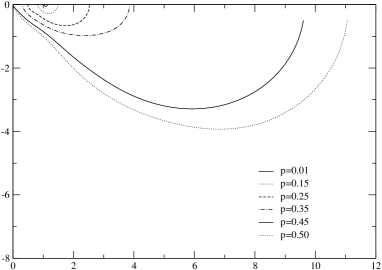
Figure 5: Nyquist diagrams, i.e. a plot of $Im(Z(\omega))$ vs. $Re(Z(\omega))$ with $\omega$ as a parameter, for 2D and 3D hypercubic resistor lattices, doped with various concentrations $p$ of capacitor bonds.

As a first application, Fig. 5 illustrates the Nyquist diagrams obtained for a square and a cubic lattice of resistors ($\sigma_{0}=R^{-1}$) which are replaced (doped) with a probability (concentration) $p$ by capacitors ($\sigma_{1}={\rm j}C\omega$).

The calculations are performed for $R=1$ and $C=1$ and lattice sizes of $12\times 12$ in 2D and $8\times 8\times 8$ in 3D. Since individual calculations for a random distribution are meaningless, averages are taken over a thousand samples for each density $p$, with $p$ varying from low density $p=0.01$ to the percolation threshold $p\simeq p_{c}$ (with the thresholds $p_{c}=0.5$ in 2D and $\simeq 0.25$ in 3D up to finite size corrections).

Fig. 5 shows that for a very small amount of capacitors ($p=0.01$), the Nyquist diagram is a perfect semi-circle centered on the value $R$ corresponding to the DC resistivity of the sample.

Figure 6: Simple electronic representations and their schematic Nyquist diagrams. The upper figure represents a 2D network where the conductors percolate. The second figure corresponds to the same situation when the insulators percolate. The last one is a model for a 3D system, with probability p such that conductors and insulators simultaneously percolate.

This can be interpreted in terms of a single capacity in parallel to a resistance, a system which is governed by a single time constant $\tau=RC$ (see Fig. 6a). For increasing $p$, the radius of the semi-circle becomes larger. As the percolation threshold is approached (at which the two electrodes would be connected by a percolating path of capacitors), a distortion of the semi-circle becomes perceptible at high frequency (i.e. close to the origin). This can be understood since the impedance of a single capacitor vanishes at infinite frequency (see Fig. 6b).

In 2D, where necessarily either capacities or resistances percolate (except for finite size effects which are compensated by averaging over many samples), all Nyquist diagrams can be interpreted qualitatively by the phenomenological model of Fig. 6. If the resistances percolate (see Fig. 6a), the impedance corresponds at low frequency to $R_{1}$ and $R_{2}$ in series, thus equaling $R_{1}+R_{2}$, whereas at high frequency the impedance is given by $R_{2}$ alone since $C_{1}$ has zero impedance. By contrast, if the capacities percolate, the equivalent phenomenological circuit is shown in Fig. 6b. At high frequency, the circuit’s impedance is governed by the two capacities in series and thus zero; at low frequency, by contrast, the real part is given by $R_{1}$ while the capacities insulating behaviour gives rise to an infinite imaginary part.

In 3D, the behaviour is radically different from the 2D case: a second semi-circle ending at the origin $Z=0$ appears in Fig. 5b as the percolation threshold $p_{c}=0.2488126$ Lore is approached from below. It is a signature of growing clusters in which capacities percolate, but which are still embedded in a resistor-dominated environment (see Fig. 6c for an illustration of such a cluster). The ratio of the radii of the two semi-circles is related to the percolation probability for a finite size sample. Above $p_{c}$ both species may percolate simultaneously. The resulting Nyquist diagram contains a single structure which is albeit more complicated than a simple semi-circle, since it is determined by a whole set of time constants deforming the diagram close to the origin (i.e. at high frequency).

5 Conclusion

As shown in Ref. Vinograd ; Sarych , the exact numerical renormalization (ENR) method allows for the calculation of the impedances of disordered networks, and is particularly well adapted if one species dominates the network. In the present work, we argue that this method is very competitive, since the formalism is simple and easy to implement, and remains numerically efficient even far from its privileged domain of application. The spectral method, on the other hand, presents advantages for repeated calculations with a great number of conductance ratios, since the spectral density of a given sample can be stored in memory for calculations of the conductances for several values of $h$ (or $\lambda$).

For the investigation of frequency-dependent quantities, these two algorithms are clearly more suitable than classical approaches such as effective medium approximation, sparse matrix method Albi , transfer matrix method Norm or the star-triangle transformation Lobb . The correctness of the ENR algorithm has been verified by comparison to small clusters (animals) whose properties can be calculated analytically.

In the present work, the ENR algorithm was used to calculate the Nyquist diagrams of two and three dimensional hypercubic lattices of randomly distributed resistors and capacities. Obviously, the results are very sensitive to the proportion of capacities to resistors, especially close to the percolation threshold. But also the dimensionality of the system plays an important role: in 2D, the Nyquist diagrams is essentially given by a single semi-circle; in 3D, by contrast, for densities just below the percolation threshold, two semi-circles are found which indicates the imminent simultaneous percolation of both components, capacities and resistors, through the system. In 2D, this scenario is ruled out, since on sufficiently large lattices, only one component may percolate at a time.

The Exact Numerical Renormalization proposed in Ref. Vinograd ; Sarych ; Tort is undoubtedly the most efficient numerical method if bonds or voids form large clusters, as in the vicinity of a percolation threshold. The algorithm also allows for a detailed analysis of the inter-bond coupling which is particularly efficient between linked bonds, but remains important for nearest neighbor bonds. Complementary information is provided by the spectral method, even though the “global animal” is in general too large for its spectrum to be interpreted in simple terms Luck ; Laurent . However, as soon as two conducting animals are separated by more than one capacity, the coupling between the animals decreases rapidly, and even if the influence of the coupling on the resonance positions is still considerable, the total spectral weight is roughly given by the sum of the individual animals’ contributions.

Further complications arise from the presence of the electrodes: the animal’s spectrum depends on its distances from the electrodes (see Tab. 2 and Tab. 3), and the resonances may be slightly altered if the animal is very close to the electrodes. For a simple animal (constituted by a few legs) and localized near the center of a large lattice (for instance $N_{x}=N_{y}=24$) the difference between the results of the ENR algorithm (where the electrodes are taken into account) and the exact analytical eigenfrequencies and their weights are almost negligible, since the shift of the resonance pulsations behaves as $1/N^{2}$.

As shown in Sect. 4, for periodic arrangements of given elementary animals, e.g. linked inductances in a capacitive array, the spectra are dominated by a few colossal resonances only. These appear at $\lambda$-values mirroring the periodicity of the arrangement and the structure of the animal itself. Only for very special arrangements, or in the very dilute limit, the whole spectrum may be completely understood on the basis of the individual animals’ spectra themselves. As these super-lattices present very interesting spectral properties, devices with specific absorption or transmission properties for electromagnetic waves might be engineered as regular arrays of metallic grains of a well-defined form on a dielectric support. In the dilute limit $p\ll 1$, the devices properties would be essentially given by the individual animals behaviour.

One can hope for very useful applications of these systems, especially in nano-technology. Moreover, progress in furtivity, active skins, giant Raman scattering could be spin-offs of a good understanding of the behavior of composite materials in an electromagnetic field (see Ref. Brou ). The knowledge of, for instance, the resonances of given patterns would allow to construct skins absorbing incident electromagnetic waves of well-defined wavelengths. By combining several animals, one could obtain an arbitrary set of resonances, leading to an arbitrary frequency response of the painted object.

Appendix A Appendix: Construction of the animals

In the following, we will present a recursive algorithm which generates all $n+1$-animals based on the entire zoo of $n$-legged animals. The basic idea is simple: it consists of adding a leg (or bond) to each $n$-animal in every possible location. However, the zoo of $n+1$-animals obtained in this manner will generally contain many identical animals. These will be eliminated by comparing each new $n+1$-animal to the already created ones, such that only one animal per species is kept. In the following, the method is applied to a 2D square lattice; a generalization to higher dimensions or different lattice types is however straightforward.

As recurrency seed, we use the only animal with “zero” legs, i.e. a point at the origin. The zoo of 1-legged animals is then obtained by adding a bond to this point, and contains two horizontal and two vertical 1-animals.

In an analogous way, the zoo of 2-legged animals can be generated by adding a further bond to these four 1-animals. Since each 1-animal has two endpoints and each of these endpoints has three vacancies at which a bond can be added, there are $4\times 2\times 3=24$ 2-animals. A closer look shows however that all 2-animals having their midpoint at the origin (i.e. 4 of the L-shaped and 2 of the straight ones) are created twice by this procedure: the full zoo of 2-legged animals thus contains only 18 species. The number of species as a function of the number of legs resulting from this recursive algorithm is listed in the third column in Table 4.

Table 4: Number of animals and species in the $n$-legged zoo as a function of $n$ and symmetry. For details, see text.

		species in the zoo
$n$	animals	symmetries:
		without	+transl.	+rot.	+mirror
1	4	4	2	1	1
2	24	18	6	2	2
3	192	88	22	7	5
4	1 920	439	88	25	16
5	22 784	2 224	372	99	55
6	311 296	11 342	1 628	416	222
7	4 796 416	58 168	7 312	1 854	950
8	82 049 024			8 411	4 265
9	1 539 876 352				19 591

By considering the system without electrodes, three more symmetries are gained which allow us to reduce the number of species in each zoo. (i) Translational invariance: in a zoo with electrodes, many animals are connected to each other by a simple shift, e.g. the two 2-animals which result from adding a horizontal bond either to the left or to the right site of the horizontal 1-animal. In an infinite lattice, such animals belong to the same species. To avoid double counting in the generation procedure, each newly created $n+1$-animal will be shifted to a well-defined place – e.g. such that its lower left corner has lattice coordinates $(0,0)$ – and will then be compared to the animals already contained in the zoo. As shown by the values in column 4 of Table 4, translational invariance reduces the number of $n$-legged species by roughly a factor $n+1$. This factor corresponds to the number of sites occupied by an $n$-animal without loops, and is thus exact for $n\leq 3$ since a loop requires at least four bonds.

(ii) Rotational invariance: by eliminating animals connected to each other via rotations by multiples of $\pi/2$, the zoos can be further reduced, as can be seen from column 5 in Table 4. The reduction with respect to the previous column approaches a factor of $4$ in the limit of large animals, $n\gg 1$. This can be easily understood because a general animal can be placed in 4 different orientations in a square lattice. This bare factor of $4$ is reduced by the presence of animals which are self-invariant under rotations by multiples of $\pi/2$. However, since the relative abundance of these self-symmetric species in the zoo decreases as the number of legs $n$ increases, the reduction factor approaches $4$ for $n\to\infty$.

(iii) Mirror symmetry: still more species can be eliminated by mirroring on the $x$-axis. As there is only one mirror axis, the number of species in the last column of Table 4 is reduced with respect to the previous column by roughly a factor of $2$ (note that mirroring on the $y$-axis is equivalent to mirroring on the $x$-axis and a subsequent rotation by $\pi$). Deviations from this factor of $2$ are again due to self-symmetric species, and diminish as the size of the animals increases.

The last column in Table 4 thus shows the number of topologically distinct species in the zoo of $n$-legged animals. These species along with the relative number of animals they contain are shown, for $n\leq 4$, in Fig. 1.

References

- (1) J.M. Debierre, P. Knauth and G. Albinet, Appl. Phys. Lett. 71 (1997), 1335.
- (2) G. Albinet, J.M. Debierre, C. Lambert and L. Raymond, Eur. Phys. J. B 22 (2001), 421.
- (3) W.H. McCrea and F.J. Whipple, Proc. Royal Soc. Edinburgh 60 (1940), 281.
- (4) F. Spitzer, Principles of Random Walk, Van Nostram inc., Princeton, (1964).
- (5) J.P. Clerc, G. Giraud, J.M. Laugier and J.M. Luck, Adv.Phys. 39 (1990), 191.
- (6) Th. Jonckheere and J.M. Luck, J. Phys. A 31 (1998), 3687.
- (7) G. Albinet and L. Raymond, Eur. Phys. J. B 13 (2000), 561.
- (8) A.P. Vinogradof and A.K. Sarychev , Sov. Phys. JETP 58 (1983), 665.
- (9) A.K. Sarychev, D.J. Bergman and Y.M. Strelniker, Phys.Rev. B 48 (1993), 3145.
- (10) L. Tortet, J.R. Gavarri, J. Musso, G. Nihoul, J.P. Clerc, A.N. Lagarkov and A. K. Sarychev, Phys. Rev. B 58 (1998).
- (11) J.P. Clerc, G. Giraud, J.M. Luck and Th. Robin, J. Phys. A 29 (1996), 4781.
- (12) J.P. Straley, J. Phys. C 12 (1979), 2143.
- (13) D.J. Bergman, Phys. Rep. 43 (1978), 377; Phys. Rev. Lett. 44 (1980), 1285; Phys. Rev. B 23 (1981), 3058; Ann. Phys. 138 (1981), 78.
- (14) C.D. Lorenz and R.M. Ziff, Phys. Rev. E 57 1 (1998), 230.
- (15) R. R. Tremblay, G. Albinet and A.-M. S. Tremblay, Phys. Rev. B 43 (1991), 11546; R. R. Tremblay, G. Albinet and A.-M. S. Tremblay, Phys. Rev. B 45 (1992), 755.
- (16) J.M. Normand, H.J. Hermann and M. Hajjar, J. Stat. Phys. 52 (1988), 441.
- (17) C.J. Lobb and D.J. Frank, Phys. Rev. B 30 (1984), 4090; D.J. Frank and C.J. Lobb, Phys. Rev. B 37 (1988), 302.
- (18) F. Brouers, S. Blacher, A.N. Lagarkov, A. K. Sarychev, P. Gadenne and V.M. Shalaev, Phys. Rev. B 55 (1997).