Energetics of metal slabs and clusters: the rectangle-box model

Abstract

An expansion of energy characteristics of wide thin slab of thickness $L$ in power of $1/L$ is constructed using the free-electron approximation and the model of a potential well of finite depth. Accuracy of results in each order of the expansion is analyzed. Size dependences of the work function and electronic elastic force for Au and Na slabs are calculated. It is concluded that the work function of low-dimensional metal structure is always smaller that of semi-infinite metal sample.

A mechanism for the Coulomb instability of charged metal clusters, different from Rayleigh’s one, is discussed. The two-component model of a metallic cluster yields the different critical sizes depending on a kind of charging particles (electrons or ions). For the cuboid clusters, the electronic spectrum quantization is taken into account. The calculated critical sizes of Ag${}_{\rm N}^{\rm 2-}$ and Au${}_{\rm N}^{\rm 3-}$ clusters are in a good agreement with experimental data. A qualitative explanation is suggested for the Coulomb explosion of positively charged Na${}_{\rm N}^{\rm n+}$ clusters at 3$\leq n\leq$5.

I Introduction

Clusters constitute a bridge between atomic, molecular and surface physics. Numerous investigations of physical properties of the low-dimensional systems are stipulated by their promising application in the nanotechnology.

Recently 14. , the work function of atomically uniform Ag films grown on Fe(100) was measured as a function of film thickness. The maxima of the work function magnitude correspond to the “magic” thicknesses. Scanning-tunneling microscopy observation of Pb nanocrystals grown on Cu(111) indicates that in the equilibrium distribution of the island heights, some heights appear much more frequently than other ones Otero . An appearance of these ‘magic” island heights on the Cu flat surface was studied by self-consistent electronic structure calculations Chulok .

Point contacts of gold bodies are investigated experimentally in Refs. 6. ; 7. during elongation of the contacts to the rupture. It is shown that oscillations of elastic constants appear simultaneously with an abrupt change in conductance. A dimensionality of a contact varies during the process of stretching. Indeed, at the moment of formation of a contact, the contact region can be represented as a slab inserted between electrodes, whereas at the moment of its rupture, the contact region becomes a wire. Thus, in the experiment we observe a transition from $2D$ (or $0D$) to $1D$ open electron system.

Analytical approaches to the determination of the density of states and the Fermi energy for metal slabs are proposed in Refs. 1. ; Nag on the basis of the free electron model. Quantization of a contact potential difference for a slab was described in Ref. 2. within the framework of the model of hard walls. Jumps of the tensile force in a point contact were explained in Refs. 3. ; 4. ; 5. . However, the work function cannot be determined in this simplest model (see review PR-2003 ).

Probably, the electron work function of a slab was calculated for the first time by Schulte Schulte . The work function magnitude showed oscillations near its average value. In Ref. Pash , the above approaches have been criticised. Detailed computations 8. ; 9. ; 10. ; Woi ; 11. ; 12. ; 13. (including ab initio calculations) performed to date do not yield an unequivocal conclusion about size dependence of the work function of isolated slabs and wires. In addition, amplitudes of the work function oscillations are larger than in experiment.

Since the work of Sattler et al. Sattler , mass-spectrometric investigations of the charging effects in cluster beams have clearly demonstrated the size-dependent Coulomb instability of clusters composed of a countable number of atoms Nah-1 ; Nah-2 ; Yannou .

Rayleigh‘s theory predicts an instability of a charged liquid sphere of $R$ radius, when the Hartree energy exceeds twice the surface energy. The critical charge is defined by the expression

$$Q_{\rm R}=\pm\sqrt{16\pi R^{\rm 3}\tau},$$ (1)

where $\tau$ is the surface tension (or stress). Recently, this criterium of stability has been confirmed in the experiment Duft for microdroplets of ethylene glycol.

Eq. (1) (i.e. Rayleigh‘s criterium) does not determine, which type of the particles charge the cluster. A metallic droplet can contain either an excess number of electrons $\Delta N_{\rm R}^{\rm e}=|Q_{\rm R}|/e$ or ions $\Delta N_{\rm R}^{\rm i}=|Q_{\rm R}|/Ze$, where $Z$ is the valence and $e$ is the elementary positive charge. Therefore, such a problem should be considered using the two-component model of a cluster in which electrons and ions are interpreted on equal footing 93 ; 1996 . A sign of the excess charge results in different size dependence, $\Delta N_{\rm e,i}\propto R$ or $\Delta N_{\rm R}\propto R^{\rm 3/2}$.

In the present work, we developed an analytical theory of size-dependent energy and force characteristics for metal slabs using an elementary one-particle approach. This simple model makes it possible to calculate the oscillatory size dependence of the work function and elastic force. Thermal effects are not considered. An assumption of the ideal plastic strain (when volume of the slab remains constant during stretching) allows for the comparison of theoretical results and experimental ones 6. .

In the framework of the two-component model, the size-dependent Coulomb instability of charged metallic clusters was described. A spectrum quantization is taken into account for a cluster having the shape of parallelepiped. The model makes it possible to study a physical origin of the instability. Theoretical results on critical sizes of different shaped charged Au, Ag and Na clusters are in agreement with experimental ones (see Refs. Nah-1 ; Yannou and referencee therein).

II SLABS: QUASICLASSICAL APPROXIMATION

II.1 Formulation of problem

We consider a thin slab with the thickness, $L_{\rm z}\simeq\lambda_{\rm F0}$ ($\lambda_{\rm F0}$ is the Fermi wavelength of electrons in a semi-infinite metal). The thickness is much smaller than other dimensions, $L_{\rm z}\ll L_{\rm x},L_{\rm y}$. Thus, the discreteness of the electron momentum components $p_{\rm x}$ and $p_{\rm y}$ can be ignored. For typical values of the electron concentration in metals, we have $\lambda_{\rm F0}\simeq$ 0.5 nm.

As a first approximation, the profile of the one-electron effective potential in the slab can be represented as a rectangular potential well of constant depth $U_{\rm 0}<0$ with dimensions $L_{\rm x}$ , $L_{\rm y}$, and $L_{\rm z}$. A solution of the three-dimensional Schrödinger equation for a quantum box is simple. An equation can be decoupled into three one-dimensional equations. Therefore it is characterized by a set of electron wave numbers $k_{\rm xj}=2\pi j/L_{\rm x}$, $k_{\rm ys}=2\pi s/L_{\rm y}$, and $k_{\rm zi}$, which are roots of the equation

$$k_{\rm zi}L_{\rm z}=-2\arcsin(k_{\rm zi}/k_{\rm 0})+\pi i,$$ (2)

where $k_{\rm 0}=\sqrt{2m|U_{\rm 0}|}$ and $m$ is the electron mass. The numbers $j,s=0,\pm 1,\pm 2,\pm 3,...$ and $i=1,2,3,...$

The set of wave numbers determines the electron energy:

$$E_{\rm p}=\frac{\hbar^{\rm 2}}{2m}\left(k_{\rm xj}^{\rm 2}+k_{\rm ys}^{\rm 2}+k_{\rm zi}^{\rm 2}\right),$$

where $p$ is the number of the electron state (the states are numbered in order of increasing of the electron energy). For a cuboid with hard walls and dimensions $L_{\rm x}$, $L_{\rm y}$, $L_{\rm z}$, we use the well-known expression

$$E_{\rm p}^{\rm\infty}=\frac{\hbar^{\rm 2}\pi^{\rm 2}}{2m}\left(\frac{j^{\rm 2}}{L_{\rm x}^{2}}+\frac{s^{\rm 2}}{L_{\rm y}^{2}}+\frac{i^{\rm 2}}{L_{\rm z}^{2}}\right),$$

where $j,s,i$ are the natural numbers.

It is convenient to use dimensionless variables by choosing $U_{\rm 0}$ as a unit of energy and $k_{\rm 0}^{\rm-1}$ as a unit of length. We introduce the following notation:

$$\xi_{\rm xj}=k_{\rm xj}/k_{\rm 0},\quad\xi_{\rm ys}=k_{\rm ys}/k_{\rm 0},\quad\xi_{\rm i}=k_{\rm zi}/k_{\rm 0},$$

$$l_{\rm x}=k_{\rm 0}L_{\rm x}/2\pi,\quad l_{\rm y}=k_{\rm 0}L_{\rm y}/2\pi,\quad l=k_{\rm 0}L_{\rm z}/\pi.$$

Note that energy can be interpreted as the square of the state vector in the $\xi-$space, $\xi_{\rm p}^{\rm 2}=\xi_{\rm xj}^{\rm 2}+\xi_{\rm ys}^{\rm 2}+\xi_{\rm i}^{\rm 2}$, with $\xi_{\rm p}\leq 1$. Eq. (2) gets a form

$$l\xi_{\rm i}=-\frac{2}{\pi}\arcsin\xi_{\rm i}+i.$$ (3)

Not only solutions of Eq. (3) but also their number are fully determined by the thickness $l$, namely, $i_{\rm F}=[l]+1$, where $[a]$ denotes the integer part of $a$.

II.2 Density of states

Let us estimate the interval $\Delta\xi$ between neighboring values of $\xi_{\rm z}$. It follows from Eq. (3) that, for sufficiently large values of $l$,

$$\Delta\xi\approx 1/l.$$ (4)

Distances between two consecutive values of $\xi_{\rm x}$ and $\xi_{\rm y}$ are small, namely, $\Delta\xi_{\rm x}=\xi_{\rm xj+1}-\xi_{\rm xj}=1/l_{\rm x}$ and $\Delta\xi_{\rm y}=1/l_{\rm y}$. For the relative values of the slab dimensions assumed by us, it can be easily found that $\Delta\xi\gg\Delta\xi_{\rm x},\Delta\xi_{\rm y}$. We see that the electron states $\left\{\xi_{\rm xj},\xi_{\rm ys},\xi_{\rm i}\right\}$ form a system of parallel planes $\xi_{\rm z}=\xi_{\rm i}$ in $\xi-$space and that the density of states on all these planes is the same and equal to

$$\sigma=2/(\Delta\xi_{\rm x}\Delta\xi_{\rm y})=2l_{\rm x}l_{\rm y}.$$ (5)

The factor $2$ takes into account two possible values of the electron spin polarization.

Electrons occupy the states, beginning from the point $\left\{0,0,\xi_{\rm 1}\right\}$, in ascending order of $\xi_{\rm p}^{\rm 2}$, i.e., of the state energy. Therefore, it appears that all occupied states lie in the $\xi$-space domain bounded by the plane $\xi_{\rm z}=\xi_{\rm 1}$ and the hemisphere of radius $\xi_{\rm F}=\sqrt{E_{\rm F}/|U_{\rm 0}|}$, where $E_{\rm F}>0$ is the Fermi energy equal to the maximum energy of occupied states.

The occupied states are distributed with density $\sigma$ over disks formed by intersections of the Fermi hemisphere with the planes $\xi_{\rm z}=\xi_{\rm i}$, $i=1,2,...,i_{\rm F}$. The area of the disk is $S_{\rm i}=\pi(\xi_{\rm F}^{\rm 2}-\xi_{\rm i}^{\rm 2})$. The number of occupied states coincides with the number of free electrons in the slab,

$$N_{\rm e}=\sigma\sum\limits_{\rm i=1}^{\rm i_{\rm F}}S_{\rm i}=2l_{\rm x}l_{\rm y}\sum\limits_{\rm i=1}^{\rm i_{\rm F}}\pi(\xi_{\rm F}^{\rm 2}-\xi_{\rm i}^{\rm 2}),$$ (6)

where $i_{\rm F}$ is the number of roots of Eq. 3.

The number of occupied states per unit volume is

$$\nu\equiv\frac{N_{\rm e}}{l_{\rm x}l_{\rm y}l}=\frac{2\pi}{l}\left(i_{\rm F}\varepsilon_{\rm F}-\sum\limits_{\rm i=1}^{\rm i_{\rm F}}\xi_{\rm i}^{\rm 2}\right),$$ (7)

where we used the notation $\varepsilon_{\rm F}\equiv E_{\rm F}/|U_{\rm 0}|=\xi_{\rm F}^{\rm 2}$.

By definition, the density of states $\rho(E)$ is the number of states per unit energy interval near the energy $E$ and per unit volume of the metal. In order to find this quantity, we write Eq. (7) in the form

$$\nu=\frac{2\pi}{l}\left(i_{\rm\varepsilon}\varepsilon-\sum\limits_{\rm i=1}^{\rm i_{\rm\varepsilon}}\xi_{\rm i}^{\rm 2}\right).$$ (8)

One can interpret $\nu$ as a number of states (per unit volume) whose energies do not exceed $\varepsilon$. In Eq. (8) $i_{\rm\varepsilon}$ is the index of the greatest of the roots of Eq. (3) satisfying the condition $\xi_{\rm i}^{\rm 2}\leq\varepsilon$.

We find from Eq. (3) that

$$i=l\xi_{\rm i}+\frac{2}{\pi}\arcsin\xi_{\rm i}.$$

Substituting here $\xi_{\rm i}$ by $\xi$, we let $\xi$ to take any value in the limits from $\xi_{\rm 1}$ to 1 and form an integer-valued increasing function $i(\xi)$ such that at the points $\xi=\xi_{\rm i}$ the value of the function is increased by one and in the intervals between these points the function does not change. Substituting $\xi=\sqrt{\varepsilon}$, we obtain

$$i_{\rm\varepsilon}=\left[l\sqrt{\varepsilon}+\frac{2}{\pi}\arcsin\sqrt{\varepsilon}\right].$$ (9)

Square brackets indicate an integer part.

By differentiating l.h.s. of Eq. (8) with respect to $\xi$ under the condition $i_{\rm\varepsilon}=const$, we find $\rho(\varepsilon)$. Using Eq. (9) and working backward through the normalizations, we obtain

$$\rho(E)\equiv\frac{1}{V}\frac{dN_{\rm e}}{dE}\\ =\frac{m}{\pi\hbar^{\rm 2}L_{\rm z}}\left[\frac{L_{\rm z}\sqrt{2mE}}{\pi\hbar}+\frac{2}{\pi}\arcsin{\sqrt{\frac{E}{|U_{\rm 0}|}}}\right],$$ (10)

where $V=L_{\rm x}L_{\rm y}L_{\rm z}$.

II.3 Size dependence of the work function

From Eq. (7), we obtain

$$\varepsilon_{\rm F}=\frac{1}{i_{\rm F}}\left(\frac{\nu l}{2\pi}+\sum_{\rm i=1}^{\rm i_{\rm F}}\xi_{\rm i}^{\rm 2}\right).$$ (11)

Using Eq. (9), we find that

$$i_{\rm F}=\left[l\sqrt{\varepsilon_{\rm F}}+\frac{2}{\pi}\arcsin\sqrt{\varepsilon_{\rm F}}\right].$$ (12)

In what follows, we assume that the electron density in the slab does not depend on its size and is

$$\frac{N_{\rm e}}{V}=\frac{k_{\rm 0}^{\rm 3}}{4\pi^{\rm 3}}\nu=\bar{n}_{\rm e}.$$ (13)

If the depth of the well is fixed, then Eq. (13) implies that $\nu=const$. The thickness dependence of the Fermi energy $\varepsilon_{\rm F}(l)$ can be found by solving the set of equations (11) and (12) under the additional condition $\nu=const$.

Substituting the expression $\bar{n}_{\rm e}\equiv k_{\rm F0}^{\rm 3}/3\pi^{\rm 2}$ into Eq. (13) ($k_{\rm F0}$ is the Fermi wave number for the semi-infinite metal), we find

$$\nu=\frac{4}{3}\pi\xi_{\rm F0}^{\rm 3},$$ (14)

where $\xi_{\rm F0}\equiv k_{\rm F0}/k_{\rm 0}$, i.e. $\nu$ is equal to doubled volume of the Fermi hemisphere in $\xi-$space in the limiting case $l\rightarrow\infty$.

Setting $i_{\rm F}=const$, from Eq. (11) we obtain

$$\frac{d\varepsilon_{\rm F}}{dl}=\frac{1}{i_{\rm F}}\left(\frac{\nu}{2\pi}+\frac{d}{dl}\sum_{\rm i=1}^{\rm i_{\rm F}}\xi_{\rm i}^{\rm 2}\right),$$ (15)

In order to see how the roots of Eq. (3) change with varying $l$, we differentiate both parts of this equation and find that

$$\frac{d}{dl}\xi_{\rm i}^{\rm 2}=-\frac{2\xi_{\rm i}^{\rm 2}}{l+\frac{2}{\pi\sqrt{1-\xi_{\rm i}^{\rm 2}}}}\leq 0.$$ (16)

Here, the equality valid only in the limit $l\rightarrow\infty$, i.e., as $\xi_{\rm i}\rightarrow 0$ for all $i$.

The disks $\xi_{\rm z}=\xi_{\rm i}$ are lowered with increasing $l$. The lowering rate decreases gradually, so that the lower disks move more slowly that the higher ones. Accordingly, the distance between the disks decreases and their number $i_{\rm F}$ grows. It is seen from Eq. (12) that this number increases by 1 each time the equality $\varepsilon_{\rm F}=\xi^{\rm 2}_{\rm i_{\rm F}+1}$ is satisfied. The process of disk lowering is accompanied by the “pulsation” of the Fermi hemisphere. Its radius $\xi_{\rm F}=\sqrt{\varepsilon_{\rm F}}$ alternately increases (as $d\varepsilon_{\rm F}/dl>0$), and decreases ( as $d\varepsilon_{\rm F}/dl<0$), having the average tendency to decrease. At $\xi_{\rm F}=\xi_{\rm i_{\rm F}+1}$ the derivative $d\varepsilon_{\rm F}/dl$ is discontinuous. The value of the jump decreases with increasing $l$.

The minimum value of $L_{\rm z}$ corresponds to the thickness equal to the atom diameter. Let us estimate the minimum value of $l$. We use $l=L_{\rm z}\sqrt{2m|U_{\rm 0}|}/(\pi\hbar)$, where $L_{\rm z}$ = 0.5 nm (it means that we have a single layer of atoms), and

$$|U_{\rm 0}|=E_{\rm F0}+W_{\rm e0},\quad E_{\rm F0}=\frac{\hbar^{2}}{2m}(3\pi^{2}\bar{n}_{\rm e})^{2/3}.$$ (17)

The work function for a semi-indefinite metal $W_{\rm 0}$ equals to 2.25 and 4.25 eV for Cs and Al, respectively Mich . As a result, we have $1.6<l_{\rm min}<3.5$. We assume henceforth the value $1/l$ to be small and apply an expansion in terms of $1/l$ for calculating of the Fermi energy.

Now we introduce the notation $\alpha\equiv 1/l$. The $\xi_{\rm i}(\alpha)$ dependence is implicitly determined by Eq. (3), which can be written as

$$\frac{\xi_{\rm i}}{\alpha}=-\frac{2}{\pi}\arcsin\xi_{\rm i}+i.$$ (18)

We look for the roots $\xi_{\rm i}$ in the form of the expansion

$$\xi_{\rm i}=\xi_{\rm i}\left|{}_{{}_{\rm\alpha=0}}\right.+\xi_{\rm i}^{\rm\prime}\left|{}_{{}_{\rm\alpha=0}}\right.\alpha+\frac{1}{2}\xi_{\rm i}^{\rm\prime\prime}\left|{}_{{}_{\rm\alpha=0}}\right.\alpha^{\rm 2}+\frac{1}{6}\xi_{\rm i}^{\rm\prime\prime\prime}\left|{}_{{}_{\rm\alpha=0}}\right.\alpha^{\rm 3}+...$$ (19)

Keeping the terms to the order of $\alpha^{\rm 3}$, we obtain the Fermi energy up to the order $\alpha^{\rm 2}$. It is seen from Eq. (18) that

$$\xi_{\rm i}\left|{}_{{}_{\rm\alpha=0}}\right.=0,\quad\xi_{\rm i}/\alpha\left|{}_{{}_{\rm\alpha=0}}\right.=i.$$ (20)

Differentiating both sides of Eq. (18) with respect to $\alpha$ and multiplying the result by $\alpha$, we obtain

$$\xi_{\rm i}^{\rm\prime}-\frac{\xi_{\rm i}}{\alpha}=-\frac{2}{\pi}\frac{1}{\sqrt{1-\xi_{\rm i}^{\rm 2}}}\alpha\xi_{\rm i}^{\rm\prime}.$$ (21)

Setting $\alpha=0$, we find

$$\xi_{\rm i}^{\rm\prime}\left|{}_{{}_{\rm\alpha=0}}\right.=i.$$ (22)

In a similar way, we obtain

$$\xi_{\rm i}^{\rm\prime\prime}\left|{}_{{}_{\rm\alpha=0}}\right.=-\frac{4i}{\pi},\quad\xi_{\rm i}^{\rm\prime\prime\prime}\left|{}_{{}_{\rm\alpha=0}}\right.=-\frac{24i}{\pi^{\rm 2}}.$$

Substituting the obtained expressions into Eq. (19), we find

$$\xi_{\rm i}=i\alpha-\frac{2i}{\pi}\alpha^{\rm 2}+\frac{4i}{\pi^{\rm 2}}\alpha^{\rm 3}+O(\alpha^{\rm 4}).$$ (23)

Now we evaluate the Fermi energy to the first order in $\alpha$. For this purpose, it suffices to keep the first two terms in Eq. (23) when substituting it into Eq. (11). Indeed, the order of magnitude of the error $\delta\xi_{\rm i}$ does not exceed $i_{\rm F}\alpha^{\rm 3}$ in this case. The error of $\xi_{\rm i}^{\rm 2}$ is $2\xi_{\rm i}\delta\xi_{\rm i}$, and its order of magnitude also does not exceed $i_{\rm F}\alpha^{\rm 3}$, since $\xi_{\rm i}\leq 1$. The error of the sum $\sum_{\rm i=1}^{\rm i_{\rm F}}\xi_{\rm i}^{\rm 2}$ is smaller than $i_{\rm F}^{\rm 2}\alpha^{\rm 3}$, and the order of magnitude of the error of the whole expression (11) does not exceed $i_{\rm F}\alpha^{\rm 3}$. Since $i_{\rm F}\simeq\sqrt{\varepsilon_{\rm F}}/\alpha$, this estimation of the Fermi energy is correct to first order in $\alpha$.

After the above-mentioned substitution into Eq. (11), we have

$$\varepsilon_{\rm F}=\frac{\nu}{2\pi}\frac{1}{i_{\rm F}\alpha}+\left(\frac{i_{\rm F}^{\rm 2}}{3}+\frac{i_{\rm F}}{2}\right)\alpha^{\rm 2}-\frac{4i_{\rm F}^{\rm 2}}{3\pi}\alpha^{\rm 3}+O(\alpha^{\rm 2}).$$ (24)

We divide the range of variation of $\alpha$ into intervals $(\alpha_{\rm i+1},\alpha_{\rm i})$, $i=2,3...$, so that $\alpha_{\rm i}\equiv 1/l_{\rm i}$ we have $i_{\rm F}=i$ inside these intervals. The values $\alpha>0.3$, which correspond to $l<l_{\rm min}$, are nonphysical. Let us find the boundaries of the intervals.

From Eqs. (23), (24) and condition $\varepsilon_{\rm F}=\xi_{\rm i+1}^{\rm 2}$ we can obtain an equation for $\alpha_{\rm i+1}$:

$$\frac{8i^{\rm 3}}{3\pi}\alpha_{\rm i+1}^{\rm 4}-\left(\frac{2i^{\rm 3}}{3}+\frac{3i^{\rm 2}}{2}\right)\alpha_{\rm i+1}^{\rm 3}+\frac{\nu}{2\pi}=0.$$ (25)

According to Descartes’ rule of signs, Eq. (25) has two real positive roots. In zeroth approximation, one of them is $\sim\sqrt{\varepsilon_{\rm F0}}/i$ and the other is of a higher order of smallness. We are interested in the first root of Eq. (25), because boundaries of the interval $(\alpha_{\rm i+1},\alpha_{\rm i})$, with constant $i_{\rm F}$ inside, are determined by this root. The boundaries are

$$\alpha_{\rm p}=\frac{1}{i}\sqrt{\varepsilon_{\rm F0}}+\frac{1}{2i^{\rm 2}}\sqrt{\varepsilon_{\rm F0}}\left(\frac{4}{\pi}\sqrt{\varepsilon_{\rm F0}}\mp 1\right).$$ (26)

The minus sign corresponds to $p=i+1$, and the plus sign to $p=i$. Thus, the width of the interval $(\alpha_{\rm i+1},\alpha_{\rm i})$ decreases as $1/i^{\rm 2}$ with increasing $i$ (or $l$), since $\alpha_{\rm i}-\alpha_{\rm i+1}=\sqrt{\varepsilon_{\rm F0}}/i^{\rm 2}$.

Unexpectedly, the examination of function $\varepsilon_{\rm F}(\alpha)$ indicates the insufficiency of its approximation by the expression (24). This expression is stair-like function, i.e., it is constant within intervals $(\alpha_{\rm i+1},\alpha_{\rm i})$, where $i_{\rm F}=i$. It can be explained by the fact that $\alpha_{\rm i+1}$ and $\alpha_{\rm i}$ differ in the second order of smallness, and after substituting into (24) they give the same results (of course, terms of the order more than first must be omitted in the resultant expression). A numerical calculation of $\varepsilon_{\rm F}$ by the formula (24) leads to the error that is associated with an incorrect consideration for terms of the order more than first and gives an appearance of the oscillatory dependence $\varepsilon_{\rm F}(l)$.

In order to take the terms $\sim\alpha^{2}$ on the right-hand side of Eq. (24) into account, we must include the following terms, which were earlier neglected:

$$\frac{1}{6}\alpha^{\rm 2}-\frac{2i_{\rm F}}{\pi}\alpha^{\rm 3}+\frac{4i_{\rm F}^{\rm 2}}{\pi^{\rm 2}}\alpha^{\rm 4}.$$ (27)

In this case, the $\varepsilon_{\rm F}(l)$ dependence is represented by a concave curve in each interval $(l_{\rm i},l_{\rm i+1})$, $i=2,3,...$ ($l_{\rm i}=1/\alpha_{\rm i}$).

At the points $l=l_{\rm i}$, the derivative $d\varepsilon_{\rm F}/dl$ is discontinuous and its jump is $-2{\varepsilon_{\rm F0}}^{\rm 3/2}/i^{\rm 2}$. To the left from this point, the function grows, and to the right from it, the function decreases. The jump in the derivative results in the appearance of cusps in the plot. The sharpness of the cusps decreases with increasing $i$.

For large values of $l$, Eq. (12) can be written as

$$i_{\rm F}=\frac{\sqrt{\varepsilon_{\rm F0}}}{\alpha}+O(\alpha^{\rm 0}).$$ (28)

Substitute Eq. (28) into Eq. (24) and using conventional units, we obtain

$$E_{\rm F}=E_{\rm F0}+\frac{\pi\hbar}{2}\sqrt{\frac{E_{\rm F0}}{2m}}\left(1-\frac{8}{3\pi}\sqrt{\frac{E_{\rm F0}}{|U_{\rm 0}|}}\right)\frac{1}{L_{\rm z}}.$$ (29)

The expression in the brackets is positive, i.e., asymptotically, we always have $E_{\rm F}>E_{\rm F0}$.

In this model, the work function is defined as:

$$W_{\rm e}=-U_{\rm 0}-E_{\rm F},$$ (30)

and it is easy to see that $W_{\rm e}<W_{\rm e0}$. A role of the size dependence of the bottom of the potential well $U(L_{\rm z})$ will be discussed later.

II.4 Deformation force

In order to calculate force characteristics, we must find the size dependent electron kinetic energy. We denote the total kinetic energy of the electrons by $\varepsilon\equiv K/|U_{\rm 0}|$.

As noted above, the one-electron kinetic energy $\varepsilon_{\rm p}$ is numerically equal to the square of the radius-vector of the point in $\xi-$space. The contribution from the corresponding element $dS$ of the disk to the total kinetic energy is $d\varepsilon=\varepsilon_{\rm p}\sigma dS$, where the density of states $\sigma$ is defined by Eq. (5). Next, we must integrate over the disk area and sum the contributions from all disks.

We introduce the notation $\rho\equiv(\xi_{\rm xj}^{\rm 2}+\xi_{\rm ys}^{\rm 2})^{\rm 1/2}$. The maximum value of $\rho$ in the $i$-th disk is equal to the disk radius $\rho_{\rm i}=(\varepsilon_{\rm F}-\xi_{\rm i}^{\rm 2})^{\rm 1/2}$. We have

$$\varepsilon=4\pi l_{\rm x}l_{\rm y}\sum\limits_{\rm i=1}^{\rm i_{\rm F}}\int\limits_{\rm 0}^{\rm\rho_{\rm i}}d\rho\rho(\xi_{\rm i}^{\rm 2}+\rho^{\rm 2})\\ =\pi l_{\rm x}l_{\rm y}\left(i_{\rm F}\varepsilon_{\rm F}^{\rm 2}-\sum\limits_{\rm i=1}^{\rm i_{\rm F}}\xi_{\rm i}^{\rm 4}\right).$$ (31)

Performing the summation, we find

$$\varepsilon=\pi l_{\rm x}l_{\rm y}\left(\left(\frac{\nu^{\rm 2}}{4\pi^{\rm 2}}\frac{1}{i_{\rm F}\alpha^{\rm 2}}+\frac{\nu}{3\pi}i_{\rm F}^{\rm 2}\alpha-\frac{4}{45}i_{\rm F}^{\rm 5}\alpha^{\rm 4}\right)\right.\\ +\left.\left(\frac{\nu}{2\pi}i_{\rm F}\alpha-\frac{4\nu}{3\pi^{\rm 2}}i_{\rm F}^{\rm 2}\alpha^{\rm 2}-\frac{1}{6}i_{\rm F}^{\rm 4}\alpha^{\rm 4}+\frac{32}{45\pi}i_{\rm F}^{\rm 5}\alpha^{\rm 5}\right)\right)+O(\alpha).$$ (32)

The asymptotic form of this expression in conventional units is

$$K=\frac{3}{5}N_{\rm e}E_{\rm F0}+\frac{3\pi\hbar}{8}N_{\rm e}\sqrt{\frac{E_{\rm F0}}{2m}}\left(1-\frac{32}{15\pi}\sqrt{\frac{E_{\rm F0}}{|U_{\rm 0}|}}\right)\frac{1}{L_{\rm z}}.$$ (33)

Let us discuss the origin of the different terms in Eq. (33).

The first term in Eq. (33) is the kinetic energy in the case, when the slab thickness $L_{\rm z}$ is comparable to other dimensions. The distance between the disks in $\xi-$space in this case is so small that the summation in Eq. (31) can be replaced by integration.

The second term in the brackets in Eq. (33) appears for a finite well depth. This correction is rather important and makes a contribution of about 50%. In contrast to the case of an infinite well, electron localization in a well of finite depth is not strict, therefore, the kinetic energy in the latter case is smaller.

In order to compare our results with the experimental data 6. ; 7. , we find the oscillating electron contribution to the elastic force under the conditions of ideal plastic strains, i.e., in the case where total volume of the slab is conserved:

$$f_{\rm z}=-(\partial\varepsilon/\partial l_{\rm z})_{\rm V}.$$

This part of the force has no relation to the phases of stretching that are accompanied by a change in volume. It rather determines the variation in slab elastic properties as the slab thickness is varied. This force depends on the number of particles in the slab, therefore, it is convenient to consider the force normalized by $N_{\rm e}$,

$$\frac{F_{\rm z}}{N_{\rm e}}=\frac{\hbar^{\rm 2}}{2m}\left(-\frac{\pi\bar{n}_{\rm e}}{i}+\frac{2\pi^{\rm 2}}{3}\frac{i^{\rm 2}}{L_{\rm z}^{\rm 3}}-\frac{\pi^{\rm 3}}{9\bar{n}_{\rm e}}\frac{i^{\rm 5}}{L_{\rm z}^{\rm 6}}+\pi^{\rm{}^{\rm 2}}\frac{i}{L_{\rm z}^{\rm 3}}\right.\\ -\left.\frac{4\pi^{\rm 2}}{k_{\rm 0}}\frac{i^{\rm 2}}{L_{\rm z}^{\rm 4}}+\frac{5\pi^{\rm 3}}{24\bar{n}_{\rm e}}\frac{i^{\rm 4}}{L_{\rm z}^{\rm 6}}+\frac{16\pi^{\rm 3}}{15\bar{n}_{\rm e}k_{\rm 0}}\frac{i^{\rm 5}}{L_{\rm z}^{\rm 7}}\right).$$ (34)

III CHARGED CLUSTERS

III.1 Two-component model: asymptotic expressions

Let us consider now a neutral cluster, which contains $N_{\rm e}/Z=N_{\rm i}=N$ atoms. Total energy of a cluster, charged by $\Delta N_{\rm e}\ll N_{\rm e}$ electrons, can be written as 16. :

$$\tilde{E}_{\rm N_{\rm e}+\Delta N_{\rm e}}=\tilde{E}_{\rm N_{\rm e}}+\mu_{\rm e}\Delta N_{\rm e}+\frac{(-e\Delta N_{\rm e})^{\rm 2}}{2C},$$ (35)

where $\mu_{\rm e}$ is the electron chemical potential. A cluster can retain the excess electrons $\Delta N_{\rm e}$ only when its energy in this state is lower than the energy in the state with $N_{\rm e}+\Delta N_{\rm e}-1$ electrons. By our definition, the number of electrons in a cluster is critical, if the number of electrons $\Delta N_{\rm e}^{\rm*}$, for which the reaction

$$M_{\rm N_{\rm i}}^{\rm(\Delta N_{\rm e}^{\rm*})-}\rightleftarrows M_{\rm N_{\rm i}}^{\rm(\Delta N_{\rm e}^{\rm*}-1)-}+e^{\rm-}$$

is reversible, and the ionization potential of the cluster, $IP^{\rm*}>0$, tends to zero

$$\Delta\tilde{E}(\Delta N_{\rm e}^{\rm*})=\tilde{E}_{\rm N_{\rm e}+\Delta N_{\rm e}^{\rm*}-1}-\tilde{E}_{\rm N_{\rm e}+\Delta N_{\rm e}^{\rm*}}\equiv IP^{\rm*}\rightarrow 0.$$ (36)

We note that the addition of one more surplus electrons to $\Delta N_{\rm e}^{\rm*}$ is possible only in a metastable state, because the affinity of this electron is

$$EA^{\rm*}=\tilde{E}_{\rm N_{\rm e}+\Delta N_{\rm e}^{\rm*}}-\tilde{E}_{\rm N_{\rm e}+\Delta N_{\rm e}^{\rm*}+1}\\ =-\mu_{\rm e}-\frac{e^{\rm 2}}{2C}(2\Delta N_{\rm e}+1)<0.$$ (37)

In any case, the relation

$$IP^{\rm*}-EA^{\rm*}=\frac{e^{\rm 2}}{C}$$

is valid. When $\Delta N_{\rm e}>\Delta N_{\rm e}^{\rm*}$, the cluster is overcharged. The surplus electrons are separated from the free states by a potential barrier and they can be in the metastable state for some time. The lifetime of each electron is determined by specific conditions in the nonequilibrium system.

Using Eqs. (36) and (35), we obtain for the critical excess electron charge

$$\Delta N_{\rm e}^{\rm*}=\frac{W_{\rm e0}C-\mu_{\rm e1}}{e^{\rm 2}}+\frac{1}{2},$$ (38)

where $W_{\rm e0}=-\mu_{\rm e0}$ is the electron work function for a flat surface, $\mu_{\rm e}=\mu_{\rm e0}+\mu_{\rm e1}/R$, and $\mu_{\rm e1}/R$ is the first curvature correction term in the electron chemical potential of a metal sphere of $R=N^{\rm 1/3}r_{\rm 0}$ radius with the notation $r_{\rm 0}$ for the mean ion spacing.

Let us consider now a positively charged cluster of metal, which contains $N_{\rm e}=ZN_{\rm i}$ electrons and $N_{\rm i}+\Delta N_{\rm i}$ ions. This situation is similar to that one when the droplet with $N_{\rm i}$ ions “contains” $\Delta N_{\rm e}<0$ lacking electrons. In this connection, $\Delta N_{\rm e}$ has to be divisible by $Z$.

The energy of charged cluster $\tilde{E}_{\rm N_{\rm i}+\Delta N_{\rm i}}$ is related to the energy of a neutral cluster in the following way

$$\tilde{E}_{\rm N_{\rm i}+\Delta N_{\rm i}}=\tilde{E}_{\rm N_{\rm i}}+\mu_{\rm i}\Delta N_{\rm i}+\frac{(+eZ\Delta N_{\rm i})^{\rm 2}}{2C}.$$ (39)

As in Eq. (35) the most essential size dependence is due to the self-repulsion of the surface charge $+eZ\Delta N_{\rm i}$. Actually, the ions are not mobile and the redistribution in the electronic subsystem mimics the distribution of an excess positive charge.

The change in the total energy, associated with the detachment of $\Delta N_{\rm i}-$th ion, is

$$\Delta\tilde{E}(\Delta N_{\rm i})=\tilde{E}_{\rm N_{\rm i}+\Delta N_{\rm i}-1}-\tilde{E}_{\rm N_{\rm i}+\Delta N_{\rm i}}\\ =-\mu_{\rm i}-\frac{e^{\rm 2}Z^{\rm 2}}{2C}(2\Delta N_{\rm i}-1).$$ (40)

A cluster with charge $+eZ\Delta N_{\rm i}$ can exist in equilibrium only if $\Delta\tilde{E}(\Delta N_{\rm i})>0$. So the number of ions $\Delta N_{\rm i}^{\rm*}$ in a cluster is critical, if the reaction

$$M_{\rm N_{\rm i}+\Delta N_{\rm i}^{\rm*}}^{\rm Z(\Delta N_{\rm i}^{\rm*})+}\rightleftarrows M_{\rm N_{\rm i}+\Delta N_{\rm i}^{\rm*}-1}^{\rm Z(\Delta N_{\rm i}^{\rm*}-1)+}+M_{\rm 1}^{\rm Z+}$$

is reversible. In this case we have

$$\Delta N_{\rm i}^{\rm*}=\frac{W_{\rm i0}C-\mu_{\rm i1}}{(Ze)^{\rm 2}}+\frac{1}{2},$$ (41)

where $W_{\rm i0}=-\mu_{\rm i0}$ is the ion work function for a plane surface. For a sphere of radius $R=(N_{\rm i}+\Delta N_{\rm i})^{\rm 1/3}r_{\rm 0}$, using sum rules 93 , we can write

$$\mu_{\rm i1}=\frac{2\gamma}{\bar{n}_{\rm e}}-\mu_{\rm e1},$$ (42)

where $\gamma$ is the surface energy per unit area. For materials under the study $\mu_{\rm e1}\simeq$ 1.9 eV$\times a_{\rm 0}$ 1996 ; 94ab .

If $\Delta N_{\rm i}>\Delta N_{\rm i}^{\rm*}$, the cluster emits a surplus ion, passing into the state with lower energy. This approach corresponds to the consideration of the droplet as a two-component electron-ion system.

The work function of single-charged ion can be expressed by means of the Born cycle 168 using the ionization potential of single atom $IP(1)$, cohesive energy $\varepsilon_{\rm coh0}$, and work function for a flat surface $W_{\rm e0}$:

$$W_{\rm i0}=\varepsilon_{\rm coh0}+IP(1)-W_{\rm e0}.$$ (43)

For Pb $\varepsilon_{\rm coh0}$ = 1.5 eV, $W_{\rm e0}$ = 4.0 eV, $IP(1)$ = 7.4 eV, and we get $W_{\rm i0}$ = 4.9 eV. When $R=12a_{\rm 0}$, the critical charge is equal to +2.7$e$. This estimation is in a good agreement with experimental data Sattler and with the results of more complicated self-consistent calculations Nah-1 .

Our approximation assumes that the shape of a cluster is unvariable during its charging. Eq. (38) for $\Delta N_{\rm e}^{\rm*}$ and Eq. (41) for $\Delta N_{\rm i}^{\rm*}$ take into account electron and ion emission and distinguish between them. It is due to the necessity to expend the energy on the embedding of a particle of this kind into the cluster and on the redistribution of its charge over the surface. Such a mechanism of the Coulomb instability can be introduced as an alternative to Rayleigh‘s one. Estimates show that $\Delta N_{\rm R}>\Delta N_{\rm i}^{\rm*}>\Delta N_{\rm e}^{\rm*}$, i.e. during the charging, rather the single-electron/ion emission occurs than Rayleigh s instability. For small clusters, the energy quantization is important.

III.2 Quantum spectra

The shape of real charged clusters seldom looks like a sphere (e.g. see 15ao ; dots ), therefore it is convenient to determine the electron spectrum using the parallelepiped model. The allowable levels form a discrete spectrum. Wave vector components are evaluated by solutions of Eq. (2) for each directions. In order to separate real levels from virtual ones we introduce the following condition:

$$k_{\rm p}/k_{\rm 0}<1.$$ (44)

Using the perturbation theory, Eq. (2) can be reduced to the infinite well problem KK-66 . Three relations of identical form determine wave numbers, for example,

$$k_{\rm xj}=k_{\rm xj}^{\rm\infty}+\Delta k_{\rm xj},\quad\zeta\equiv|\Delta k_{\rm xj}/k_{\rm xj}^{\rm\infty}|\ll 1,$$ (45)

where $k_{\rm xj}^{\rm\infty}=\pi j/L_{\rm x}$ is the solution at $k_{\rm 0}\rightarrow\infty$. Substituting Eqs. (45) into Eq. (2), we obtain in the first approximation for a cube $\zeta=-2/k_{\rm 0}L$ and the energy spectrum

$$E_{\rm p}=\frac{\hbar^{\rm 2}\pi^{\rm 2}}{2mL^{2}}(j^{\rm 2}+s^{\rm 2}+i^{\rm 2})(1+2\zeta+O(\zeta^{\rm 2})).$$ (46)

One more alternative expression can be derived from Eq. (2) under the condition (44):

$$E_{\rm p}\simeq\frac{\hbar^{\rm 2}\pi^{\rm 2}}{2m}\left(\frac{k_{\rm 0}}{2+k_{\rm 0}L}\right)^{\rm 2}(j^{\rm 2}+s^{\rm 2}+i^{\rm 2}).$$ (47)

On the one hand, in a neutral cube number of electrons is given, on the other hand it is determined by sum 2$\sum_{\rm p}\delta(E-E_{\rm p})$ over all occupied levels taking into account twofold spin degeneracy. Filling levels by electrons we find a highest occupied state, $E^{\rm HO}<0$, counted off from the vacuum level. Following the Koopmans‘ theorem the ionization potential of a cubiform cluster can be determined as

$$IP=-E^{\rm HO}+\frac{e^{\rm 2}}{2C}.$$ (48)

IV RESULTS AND DISCUSSION

We performed calculation for slabs of trivalent Al, monovalent Au and Na with electron concentration $\bar{n}_{\rm e}=3/4\pi r_{\rm s}^{\rm 3}$, where $r_{\rm s}=$ 2.07, 3.01 and 3.99 $a_{\rm 0}$, respectively. The work function values for semi-infinite metals, which we used, are $W_{\rm e0}=$ 4.25, 5.15 (or 4.3) and 2.7 eV Mich ; 39 .

Figure 2 shows the results of calculation of the thickness dependence of the work function for extended isolated slabs. The inequality $W_{\rm e}<W_{\rm e0}$ is satisfied for the whole thickness range. The values of the largest oscillations of the work function are about 0.1 – 0.2 eV. This size dependence is in a general agreement with the experimental results 14. and self-consistent calculations for extended thin Al slabs 12. and cylindrical Al and Na wires 11. ; 13. . However, there is a disagreement with the results of 8. ; 9. ; 10. ; Woi .

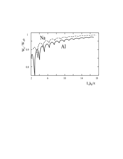
Figure 1: Size dependence of the work function for metallic slabs.

Comparing $W_{\rm e}(L)$ for various metals, it is easily seen that all differences are determined by the values of $r_{\rm s}$. For aluminum (with the smallest $r_{\rm s}$), the amplitude of oscillations of the work function $W_{\rm e}/W_{\rm e0}$ is the largest, the period $\Delta L$ is the smallest, and position $L_{\rm i}$ of the cusps are displaced to the left. These features are well described by the approximate relations $1-W_{\rm e}/W_{\rm e0}\sim 1/r_{\rm s}L$, $\Delta L\sim r_{\rm s}$, and $L_{\rm i}\sim ir_{\rm s}$ ($i$ is the number of subband), which follow from Eqs. (26) and (29).

In order to clarify the role of the thickness dependence of the bottom of the well (see Eq. (17)), we consider the data presented in Table 1. These data are extracted from the results of the self-consistent calculations performed in 15. . In that work, the electron energy spectrum was calculated for a self-consistent spherical potential whose form was far from being rectangular. In the rectangle-box model the position of the first occupied level $E_{0}$ varies in accordance with the position of flat bottom of the potential well. As the well width is large (i.e., as $N\rightarrow\infty$), this level is “lowered” to the bottom. Hence, we can obtain quite reliable information about the size dependence of the depth of the rectangular well by determining the confinement behavior of the lowest level in the potential profile corresponding to the spherical cluster.

Table 1: The energy of the first occupied state, $E_{\rm 0}<0$, in spherical clusters Na_N calculated by Ekardt 15. .

N	18	20	34	40	58	68	90
$-E_{\rm 0}$ [eV]	5.10	5.15	5.41	5.41	5.59	5.53	5.76
N	92	106	132	138	168	186	198
$-E_{\rm 0}$ [eV]	5.63	5.64	5.86	5.79	5.91	5.92	5.81

This dependence is almost monotonic and asymptotically weak. Moreover, it does not compete with the thickness dependence of the Fermi energy in Eq. (30) and gives a minor contribution to Eq. (29). Taking into account the dependence $U(L)$ in Eq. (30) leads to strengthening of the inequality $W_{\rm e}<W_{\rm e0}$.

When the slab is inserted into contact with the electrodes, the electron chemical potentials are equalized and the electronic system should be considered as an open system with $W_{\rm e}(L)=W_{\rm e0}$. The electrical neutrality of the slab cluster is broken, and the part $\delta N_{\rm e}>0$ of the electron liquid passes out to the bath. As a result, a contact potential difference $\delta\phi$ appears.

In order to determine the contact potential difference, we consider energy cycles, in which electrons are transferred first to infinity and then to the electrodes. By analogy with Eq. (36), we express the ionization potential of the slab, having charge $+e\delta N_{\rm e}$, as

$$IP=E_{\rm N_{\rm e}-\delta N_{\rm e}-\Delta}-E_{\rm N_{\rm e}-\delta N_{\rm e}}\\ =W_{\rm e}\Delta+\frac{e^{\rm 2}}{2C}((\delta N_{\rm e}+\Delta)^{\rm 2}-\delta N_{\rm e}^{\rm 2})$$ (49)

and write the electron affinity of the bath for the charge $-e\Delta$ as $EA=W_{\rm e0}\Delta$. Equating these two quantities, we obtain

$$W_{\rm e0}-W_{\rm e}-\frac{e^{\rm 2}}{2C}(2\delta N_{\rm e}+\Delta)=0,$$ (50)

where C is the sample capacitance.

We note that $\Delta$ can be infinitesimal, since an electron can pass through the contact only partially (i.e., it can be detected on both sides of the geometrical contact with a nonzero probability). $\delta N_{\rm e}$ can be considered as a smoothly varying quantity. This situation is typical for one-electron devices 17. .

We also assume that $C$ corresponds to the total capacitance of the both contacts. The validity of this assumption depends on the sample geometry and electromagnetic environment. This is not true for a spherical cluster in contact with electrodes, but it is valid for a cubiform cluster or a slab n1 . Neglecting environment and setting $C=e\delta N_{\rm e}/\delta\phi$, $\delta N_{\rm e}\ll N_{\rm e}$, and $\Delta\rightarrow 0$, we obtain from Eq. (50)

$$\delta\phi=(W_{\rm e0}-W_{\rm e})/e.$$ (51)

Now the energy spectrum of the $N_{\rm 1}=N_{\rm e}-\delta N_{\rm e}$ electrons that remain in the slab must be found for the rectangular potential well of changed depth $U_{\rm 0}-e\delta\phi$. The total kinetic energy $K_{\rm 1}$ of the remaining electrons can be determined in the same way as for an isolated slab but with changed energy spectrum and number of electrons. For the oscillating part of the elastic force, we have $F_{\rm z1}=-\left(\partial\Omega/\partial L_{\rm z}\right)_{\rm V}$, where $\Omega=K_{\rm 1}+W_{\rm e0}N_{\rm 1}$ is the thermodynamic potential.

Using the data from Fig. 1, we can also determine the contact potential difference $\delta\phi$. This potential difference produces a negative shift of the well depth (for the thinnest slab, it attains 0.5 – 1 eV). This leads to a displacement of density of states to values corresponding to greater thicknesses. The stretched sample acts as an “electron pump” with respect to the electrodes, alternately ejecting electronic liquid and drawing it back.

In Fig. 2, we show the part of the elastic force that is due to the quantization. As can be seen from this figure, the amplitude of the force oscillations depends strongly on $r_{\rm s}$. For sodium, the oscillation amplitude is 8 times smaller than that for Aluminum. The character of this dependence can be determined from Eq. (34): $(F_{\rm z}/N_{\rm e})_{\rm i}\sim ir_{\rm s}^{\rm 3}$. Our estimations showed that, for a slab in a contact, force oscillations are analogous in shape and amplitude.

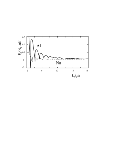
Figure 2: Size dependence of the oscillating component of elastic force $F_{\rm z}/N_{\rm e}$ for metallic slabs.

The first maximum of the oscillating part of the force $F_{\rm z}/N_{\rm e}$ for Au (corresponding to a slab thickness of one monolayer) is 0.2 nN, i.e., it is much smaller than the experimental value for a wire, which is equal to 1.5 nN 2. . This difference can be explained by both the difference in the dimensionality of the electron gas in a wire and in a slab and the effect of current flowing through a contact estimated in Ref. 20. and discussed in Ref. Vetra . Note that there are no experimental results for slabs.

For the case of aluminum cluster, let us apply analytical approach of the previous section. Size dependences of the ionization potential (48) calculated for the cubiform clusters Al_N are shown in Fig. 3. Here we use spectra, which are determined by Eqs. (2), (46), and (47). For the $N$ range (10, 3000), calculations designate an essential role of spectrum quantization even for large clusters. Magic numbers obtained are close to those found experimentally 38 . They are different in the case of single valence sodium clusters.

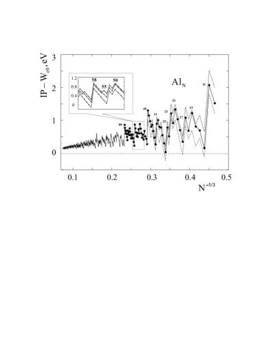
Figure 3: Size dependences of the first ionization potential (48) of Al_N clusters. Solid, dashed, and dot-dashed lines indicate the dependences determined according to solutions Eqs. (2), (46), and (47), respectively. Numbers at the top correspond to the numbers of atoms in the cluster.

Beginning from one hundred atoms, calculations of the spectrum based on approximate expressions (46) and (47) give quite reasonable results. However, their inaccuracy results in the level hierarchy differing from that determined from Eq. (2). There is a difference between spectra calculated by Eqs. (46) and (47) for $N$ values near $N=58$ (see insert in Fig. 3) n2 .

At the next step we investigate the ionization potential of a cluster as a function of its shape. We assume that shape of a cuboid cluster varies from strongly flattened to elongated. Thus, we have a monatomic slab of thickness $L$ at the beginning and a monatomic chain of length $L$ at the end. During this evolution, the sample volume is supposed to be constant and equal to 4 nm³.

We divide the range of the size variation into 10³ intervals and find the spectrum for each of them using Eq. (2). We exchange a capacitance of the parallelepiped by capacitance of equivalent spheroid in the ionization potential (48). The size dependence of the capacitance has a minimum for a sphere. In the limiting cases of the slab and the wire of monoatomic thickness capacitances are approximately twice and sevenfold larger, respectively.

Figure 4 displays the behavior of the electron work function and the ionization potential of the isolated sodium samples of varying shapes. The inequality $-E^{\rm HO}<W_{\rm e0}$ is observed to be obeyed over the whole range of the considered dimensionalities. The size dependence of energy of the first occupied state, $E_{\rm 0}(L)$, has minimum at the point corresponding to a cubiform cluster. As it can be seen, there are ranges of lengths, where $IP<W_{\rm e0}$ and $IP>W_{\rm e0}$. The inequality $IP<W_{\rm e0}$ is rather surprising. It is known from experiments that the work function $W_{\rm e0}$ of alkali metals is approximately equal to the one half of $IP$ of the atom 79a . Therefore one would expect that the value of $IP$ of a small solid sample belongs to the interval $W_{\rm e0}<IP<IP({\rm atom})$ independently of the shape of sample surface. However, the competition between the size correction $W_{\rm e}(L)$ and the $e^{\rm 2}/2C$ term in expression (48) for the ionization potential can lead to the opposite inequality.

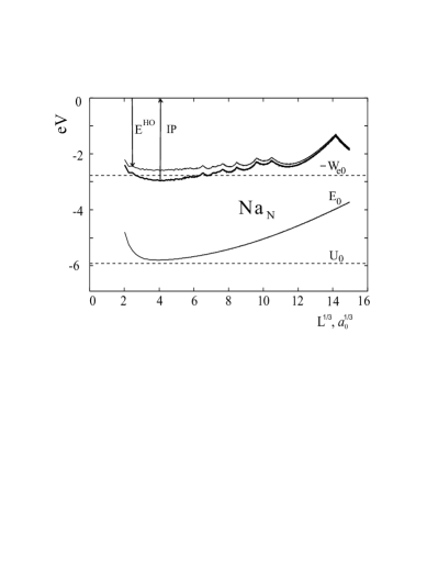
Figure 4: Evolution in the size dependence of the first ionization potential (48) of Na_N cubiform cluster with a change in the cluster shape from a slab to a wire. Dashed lines represent the bottom position of the potential well, $U_{\rm 0}$, and work function for the flat surface, $W_{\rm e0}$.

Using mass-spectrometer Yannou , minimal number of atoms $N$ have been recently determined for which an existence of stable charged clusters Au${}_{\rm N}^{\rm 2-}$ ($N>$27), Au${}_{\rm N}^{\rm 3-}$ ($N>$58), and Ag${}_{\rm N}^{\rm 2-}$ ($N>$27) is possible under the condition of a particle retaining 2 or 3 surplus electrons. This problem is inverse to the one considered above. Here $\Delta N_{\rm e}^{\rm*}$ is a parameter and $N$ is unknown.

We note that even for particles containing more than a thousand of ions the critical charge does not exceed a few units. This interesting feature is a result of the strong Coulomb repulsion of the surplus charge spread over the surface of the particle. The situation is different for atomic and molecular ions, where electrons are not collectivized.

For calculations, we use the following experimental values of surface tension: $\tau$ = 1134, 780, 191 erg/cm² for Au, Ag, and Na, respectively. Here, we assume that the surface energy equals the surface tension, while in reality these values can be considerably different from Kurb .

Rayleigh‘s expression gives numbers of atoms in the critical clusters, which are 4 – 5 times less. These numbers are $N\approx 9$ and 6, for Au${}_{\rm N}^{\rm 3-}$ and Ag${}_{\rm N}^{\rm 2-}$, respectively. In our approach the problem is reduced to the solution of the equation

$$IP^{\rm*}(\Delta N_{\rm e}^{\rm*},N)=-E^{\rm HO}(\Delta N_{\rm e}^{\rm*},N)\\ -\frac{e^{\rm 2}}{2C_{\rm\rm eff}(N)}(2\Delta N_{\rm e}^{\rm*}-1)=0.$$ (52)

Effective capacitance $C_{\rm\rm eff}=R+\delta$ is used in order to explain experimental results for charged clusters. The additional small quantity $\delta$ is caused by an increase of radius of the charging electron “cloud”. The $\delta$ value was introduced for calculations of the polarization by Snider and Sorbello 42 and the ionization potential of clusters by Perdew 211. . The averaged dependence $\delta(r_{\rm 0})=1.617+0.199(r_{\rm 0}/Z^{\rm 1/3}-2.07)$ (in bohrs) is obtained using coordinates of the image plane for various crystallographic faces 1996 , which were computed in the stabilized jellium model KiejnaW .

Note that introduction of $\delta$ to Eqs. (48) and (52) is not rigorous. This procedure accounts only for the Hartree contribution, $\delta/R^{2}$, into correction term $\sim 1/R^{2}$ in the energy $1/R-$expansion. Nevertheless, solution of Eq. (52) is responsible to the $\delta$ value n3 . With discussed modification for $IP$, Eq. (36) is adequate for explaining consecutive fotoionization acts for large clusters Al_N in the wide $N$ range (2000, 32000) Hoffmann . The use of $C_{\rm eff}=R+\delta$ makes the size monotonic component of $IP(N)$ in Fig. 3 some weaker.

The size dependence $IP^{*}(\Delta N_{\rm\rm e}^{*},N)$ calculated from relationships (52) and (38) is shown in Fig. 5. Points of the diagrams with $IP^{*}=0$ indicate $N$ values for the critical clusters. It can be seen from Fig. 5 that the quasiclassical dependence (38) and Eq. (52) with inclusion of the level quantization leads both to the better agreement with experimental data than Rayleigh‘s formula. For Au ${}_{\rm N}^{3-}$, we use the value $W_{\rm e0}$ = 5.15 eV recommended by Michaelson Mich . The Au${}_{\rm N}^{2-}$ clusters appear to be stable when $N>20$. However, with another value $W_{\rm e0}$ = 4.3 eV, proposed by Fomenko 39 , Eq. (52) gives Au${}_{\rm 27}^{2-}$ and Au${}_{\rm 110}^{3-}$ critical clusters. Specific features in the energy properties of gold clusters were noted by Garron Garron .

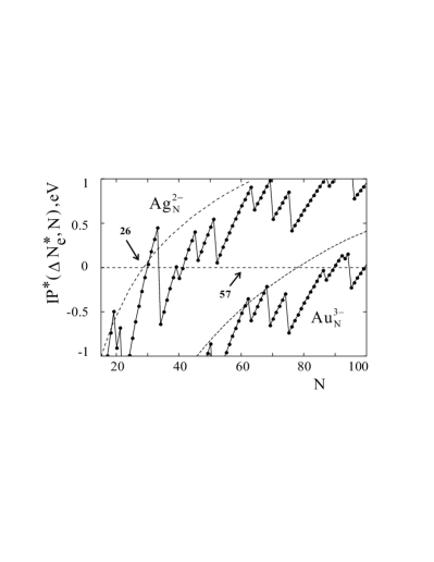
Figure 5: Size dependences of the ionization potential (52) Au${}_{\rm N}^{3-}$ and Ag${}_{\rm N}^{2-}$ clusters (solid line). Dashed lines represent the quasiclassical dependences $IP(N)$ (36). Arrows indicate the experimental critical numbers $N^{*}$.

Finally, we apply our computation procedure to the case of positively charged clusters Na${}_{\rm N}^{n+}$. Näher et al. Nah-2 determined experimentally critical numbers $N$ = 64, 123, and 208 for clusters with $n$ = 3, 4, and 5, respectively. In our model, we have $N\equiv N_{\rm i}+\Delta N_{\rm i}^{*}$ , and $n\equiv\Delta N_{\rm i}^{*}$. The critical sizes are calculated using Eqs. (41) – (43) in which we replace $W_{\rm e0}\rightarrow-E^{\rm HO}$ and eliminate $\mu_{\rm e1}$. We use $\varepsilon_{\rm coh}$ = 1.13 eV and $IP(1)$ = 5.14 eV in the calculations.

Our results for the Na${}_{\rm N}^{n+}$ clusters are presented in Fig. 6. For the small sized clusters, the situation

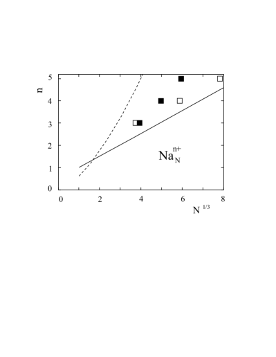
Figure 6: Critical sizes of positively charged clusters Na${}_{\rm N}^{n+}$. Solid line – quasiclassical dependence (41), dashed line – the Rayleigh dependence, ($\blacksquare$) – experiments, and ($\square$) are the results of quantization.

can be described by the Rayleigh‘s formula according to which $|Q_{\rm R}|\propto N^{1/2}$. The quasiclassical instability leads to the relationship $eZ\Delta N_{\rm i}^{*}\propto N^{1/3}$. Calculated critical sizes of the clusters occur to be overrated as compared to experimental values. From the data presented in Fig. 5, one can assume that cubiform clusters transforms predominantly into cuboids. The change in energy of the highest occupied state $E^{\rm HO}$ is significantly less than that associated with the charging due to an increase in capacitance. Elongation of clusters is accompanied also by the change in the cohesion energy (see Eqs. (41) and (43)). This is confirmed by experimental data on deformation of point contacts. A decrease in the dimensionality gives a considerable increase in strength of a contact PR-2003 . These factors can be responsible for the difference between dependences $\Delta N_{\rm i}^{*}(N)$ calculated and experimentally found.

V Summary

The problem of energetics of finite metallic systems has been considered. We have developed an analytical theory of size dependent energy and force characteristics for metal slabs by using rectangular-box model, free-electron approximation and the model of a potential well of finite depth. This approach makes it possible to calculate the oscillatory size dependence of the work function. It is concluded that the work function of low-dimensional metal structure is always smaller that that of the semi-infinite metal. The theory has been applied to calculate the elastic effects in thin metallic slab.

In the framework of the two-component model, the size dependent Coulomb instability of charged metallic clusters has been described. A mechanism of the Coulomb instability in charged metallic clusters, different from Rayleigh’s one, has been discussed. We showed that the two-component model of a metallic cluster in quasiclassical approximation leads to different critical sizes depending on a kind of charging particles (electrons or ions). For the cubiform clusters, the electronic spectrum quantization has been taken into account. The model enables us to discover the physical origin of the instability and to explain the critical sizes of charged Au${}_{\rm N}^{\rm n-}$, Ag${}_{\rm N}^{\rm n-}$ and Na${}_{\rm N}^{\rm n+}$ clusters of different shape. Results of this investigation might have an application in diagnostics of ultradispersed media, single-electronics, and in nanotechnology.

- (1) J. J. Paggel, C. M. Wei, M.Y. Chou, D.-A. Luh, T. Miller, and T.-C. Chiang, Phys. Rev. B 66 233403 (2002).
- (2) R. Otero, A. L. Vazquez de Parga, R. Miranda, Phys. Rev. B 66 115401 (2002).
- (3) E. Ogando, N. Zabala, E. V. Chulkov, and M.J. Puska, Phys. Rev. B 69 153410 (2004).
- (4) C. Untiedt, G. Rubio, S. Vieira, and N. Agraït, Phys. Rev. B 56 2154 (1997).
- (5) G. Rubio-Bollinger, S. R. Bahn, N. Agraït, K. W. Jacobsen, and S. Vieira, Phys. Rev. Lett. 87 026101 (2001).
- (6) J.P. Rogers III, P. H. Cutler, T. E. Feuchtwang, and A.A. Lucas, Surf. Sci. 181 436 (1987).
- (7) E. L. Nagaev, Phys. Rep. 222 201 (1992).
- (8) M. V. Moskalets, Pis’ma v Zh. Exp. Teor. Fiz. 62 702 (1995) [JETF Lett. 62 719 (1995)].
- (9) J. M. van Ruitenbeek, M. H. Devoret, D. Esteve, and C. Urbina, Phys. Rev. B 56 12566 (1997).
- (10) C. A. Stafford, D. Baeriswyl, and J. Bürki, Phys. Rev. Lett. 79 2863 (1997).
- (11) S. Blom, H. Olin, J. L. Costa-Kramer, N. Garcia, M. Jonson, P. A. Serena, and R. I. Shekhter, Phys. Rev. B 57 8830 (1998).
- (12) N. Agraït, A.L. Yeyati, and J. M. van Ruitenbeek, Phys. Rep. 377 81 (2003).
- (13) F. K. Schulte, Surf. Sci. 55 427 (1976).
- (14) A. M. Gabovich, L. G. Ilchenko, and E. A. Pashitskii, Fiz. Tverd. Tela 21 1683 (1979) (in Russian).
- (15) P. J. Feibelman, and D. R. Hamann, Phys. Rev. B 29 6463 (1984).
- (16) J. C. Boettger, Phys. Rev. B 53 13133 (1996).
- (17) A. Kiejna, J. Peisert, and P. Scharoch, Surf. Sci. 54 432 (1999).
- (18) K.F. Wojciechowski, Phys. Rev. B 60 9202 (1999).
- (19) N. Zabala, M. J. Puska, and R. M. Nieminen, Phys. Rev. B 59 12652 (1999).
- (20) I. Sarria, C. Henriques, C. Fiolhais, and J. M. Pitarke, Phys. Rev. B 62 1699 (2000).
- (21) E. Ogano, N. Zabala, and M. J. Puska, Nanotechnology 13 363 (2002).
- (22) K. Sattler, O. Mühlbach, and E. Recknagel, Phys. Rev. Lett. 47 160 (1981).
- (23) U. Näher, S. Bjornholm, S. Frauendorf, F. Garcias, and C. Guet, Phys. Rep. 285 245 (1997).
- (24) U. Näher, H. Göhlich, T. Lange, and T. P. Martin, Phys. Rev. Lett. 68 3416 (1992).
- (25) C. Yannouleas, U. Landman, A. Herlert, and L. Schweikhard, Phys. Rev. Lett. 86 2996 (2001).
- (26) D. Duft, H. Lebius, B. A. Huber, C. Guet, and T. Leisner, Phys. Rev. Lett. 89 084503 (2002).
- (27) I. T. Iakubov, A. G. Khrapak, V. V. Pogosov, and S.A. Trigger, Phys. Stat. Sol. b 145 455 (1988).
- (28) A. Kiejna and V. V. Pogosov, J. Phys.: Cond. Matter 8 4245 (1996).
- (29) H. B. Michaelson, J. Appl. Phys. 48 4729 (1977).
- (30) I. T. Iakubov, A. G. Khrapak, L. I. Podlubny, and V. V. Pogosov, Solid State Commun. 53 427 (1985).
- (31) M. Seidl, J. P. Perdew, M. Brajczewska, and C. Fiolhais, Phys. Rev. B 55 13288 (1997); J. Chem. Phys. 108 8182 (1998).
- (32) F. Vericat and M. P. Tosi, Nuovo Cimento D 8 105 (1986).
- (33) D. M. Wood and N. W. Ashcroft, Phys. Rev. B 25 6255 (1982).
- (34) S. M. Reimann and M. Manninen, Rev. Mod. Phys. 74 1283 (2002).
- (35) A. Kawabata and R. Kubo, J. Soc. Jap. 21 17 (1966).
- (36) V. S. Fomenko, Emission Properties of Materials (Naukova Dumka, Kiev, 1981).
- (37) W. Ekardt, Phys. Rev. B 29 1558 (1984).
- (38) D. M. Kaplan, V. A. Sverdlov, and K. K. Likharev, Phys. Rev. B 68 045321 (2003).
- (39) Near the edges of the parallelepiped, the surface distribution of excess positive charge should be similar to that for real ionization.
- (40) M. Brandbyge, J.-L. Mozos, P. Ordejon, J. Taylor, and K. Stokbro, Phys. Rev. B 65 165401 (2002).
- (41) M. Di Ventra, Y.-C. Chen, and T. N. Todorov, Phys. Rev. Lett. 92 176803 (2004).
- (42) W. A. de Heer, Rev. Mod. Phys. 65 611 (1993).
- (43) The procedure of computation of spectrum has some specific feature. We obtain the spectral term for a cuboid combining of solutions of the one-dimensional problem (see, e.g. Eq. (46)), therefore it becomes necessary to choose the combination that realizes the minimum energy.
- (44) K. Wong, S. Vongehr, and V. V. Kresin, Phys. Rev. B 67 035406 (2003).
- (45) A. Kiejna and V. V. Pogosov, Phys. Rev. B 62 10445 (2000); V. V. Pogosov and V.P. Kurbatsky, Zh. Exper. Teor. Fiz. 119 350 (2001) [JETF. 92 304 (2001)]; V. V. Pogosov, O. M. Shtepa (cond-mat/0310176).
- (46) D. R. Snider and R. S. Sorbello, Phys. Rev. B 28 5702 (1983).
- (47) J. P. Perdew, Phys. Rev. B 37 6175 (1988).
- (48) A. Kiejna, K.F. Wojciechowski, Metal Surface Electron Physics (Pergamon, Oxford, 1996).
- (49) However, this solution is not sensitive to the self-compression effect 1996 .
- (50) M. A. Hoffmann, G. Wrigge , B. von Issendorff, Phys. Rev. B 66 041404 (2002).
- (51) R. Garron, Ann. Phys. 10 595 (1965).