Nonequilibrium critical relaxation in the presence of extended defects

Abstract

We study nonequilibrium critical relaxation properties of systems with quenched extended defects, correlated in $\varepsilon_{d}$ dimensions and randomly distributed in the remaining $d-\varepsilon_{d}$ dimensions. Using a field-theoretic renormalization-group approach, we find the scaling behavior of the nonequilibrium response and correlation functions and calculate the initial slip exponents $\theta$ and $\theta^{\prime}$, which describe the growth of correlations during the initial stage of the critical relaxation, in the two-loop approximation.

I Introduction

In recent years, much attention has been attracted by the so-called short-time critical dynamics. janssen-89 ; oerding-93 ; oerding-93-2 ; kissner-92 ; oerding-95 ; chen-01 ; chen-00 ; chen-02 ; zheng-98 A thermodynamic system in a critical point is characterized by long-range correlations in equilibrium, so when such a system is quenched from a high temperature $T_{0}\gg T_{c}$ to the critical point $T_{c}$, the growth of correlations governs the relaxation process. As shown in Ref. janssen-89, , the relaxation process displays a universal scaling behavior already at times just after a microscopic time scale $t_{\mathrm{mic}}$ needed for the system to forget its microscopic details and lasts until the system has lost all memory about its macroscopic initial condition. The initial nonequilibrium stage of the critical relaxation is characterized by new critical exponents $\theta$ and $\theta^{\prime}$, which describe the behavior of the response function $G(t,t^{\prime})\propto(t/t^{\prime})^{\theta}$ for $t^{\prime}\to{0}$ and the initial increase of the order parameter $m(t)\propto t^{\theta^{\prime}}$, respectively. The critical exponents $\theta$ and $\theta^{\prime}$ depend on the dynamic universality class, hohenberg-77 and have been calculated for a number of dynamic models such as the model with a nonconserved order parameter janssen-89 (model A), the model with an order parameter coupled to a conserved densityoerding-93 (model C), and the models with reversible mode couplingoerding-93-2 (models E, F, G, and J). The universal scaling behavior of the initial stage of the critical relaxation has been verified by extensive numerical simulations.zheng-98

The influence of various kinds of disorder on phase transitions is one of the central problems in condensed-matter physics. stichcombe-83 ; chardy-96 ; pelissetto-02 ; alonso-01 ; holovatch-02 ; grinstein-76 In the present paper, we focus our attention on the nonequilibrium critical properties of systems in the presence of quenched temperaturelike disorder (for example, magnetic systems with quenched nonmagnetic impurities). In the simplest case, the disorder may be viewed as randomly distributed pointlike defects. grinstein-76 According to the Harris criterion,harris-74 the quenched uncorrelated pointlike defects change the critical behavior only if the heat capacity exponent of the pure system is positive $\alpha_{p}>0$. As a result, the pointlike disorder is relevant only for Ising-like three-dimensional ($d=3$) systems. The short-time critical behavior of systems with pointlike uncorrelated defects was studied in Refs. kissner-92, and oerding-95, . Real systems, however, often contain defects in the form of linear dislocation, planar grain boundaries, three-dimensional cavities, or other extended defects. One possibility to treat the systems with extended defects is the model suggested by Weinrib and Halperin (WH), weinrib-83 in which defects are long-range correlated and characterized by a correlation function that has a power-law decay $g(x)\propto x^{-a}$ with distance $x$. This type of disorder has a direct interpretation for integer values $a$: the case $a=d$ corresponds to uncorrelated pointlike defects, while $a=d-1$ ($a=d-2$) describes infinite lines (planes) of defects of random orientation. The statics of the WH model and its dynamics not far from equilibrium were examined by means of the renormalization-group (RG) methods to two-loop order using both the double $\varepsilon=4-d$, $\delta=4-a$ expansionkorucheva-98 and the direct calculations in $d=3$.fedorenko-00 The nonequilibrium critical relaxation of the WH model was considered only in the one-loop approximation, chen-01 although numerous investigations of pure and disordered systems performed with the use of the field-theoretic approach show that the predictions made in the one-loop approximation, especially on the basis of the $\varepsilon$ expansion, can differ from the real critical behavior. holovatch-02 ; fedorenko-00 The possible alternative to the isotropic scenario realized in the WH model is the anisotropic scenario realized in the model proposed by Dorogovtsev, dorogovtsev-80 in which defects are strongly correlated in $\varepsilon_{d}$ dimensions and randomly distributed over the remaining $\tilde{d}=d-\varepsilon_{d}$ dimensions. The case $\varepsilon_{d}=0$ is associated with uncorrelated pointlike defects, while the extended linear (planar) defects are related to the cases $\varepsilon_{d}=1$(2). The case of the noninteger value of $\varepsilon_{d}$ may be related to a system containing fractal-like defects so that $\varepsilon_{d}$ is interpreted as an effective fractal dimension of a complex random defect system.yamazaki-88 The statics and equilibrium dynamics of Dorogovtsev’s model were studied in Refs. boyanovsky-82, ; prudnikov-83, ; lawrie-84, ; blavatska-03, (for a review of the models with extended defects, see Refs. decesare-94, ; korzhenevskii-94, ; yamazaki-86, ).

In the present paper, we investigate the short-time critical dynamics of Dorogovtsev’s model with a nonconserved order parameter using a field-theoretic approach in the two-loop approximation. The paper is organized as follows. Section II introduces the model describing the critical dynamics of disordered systems with extended defects. In Sec. III, the corresponding effective field theory is renormalized up to two-loop order. In Sec. IV, we derive the asymptotic behavior of response and correlation functions and calculate the critical exponents using the Padé-Borel resummation method. The final section contains our conclusions.

II The model

In equilibrium at temperature $T$ the Hamiltonian describing the disordered systems with extended defects is given bydorogovtsev-80

$$\mathcal{H}_{V}[\phi]=\int d^{d}x\left[\frac{1}{2}\sum_{\beta=1}^{n}[\tau(\phi^{\beta})^{2}+\alpha^{2}|\nabla_{\parallel}\phi^{\beta}|^{2}\right.$$

$$+|\nabla_{\perp}\phi^{\beta}|^{2}+\left.V(\mathbf{x}_{\perp})(\phi^{\beta})^{2}]+\frac{g\alpha^{\varepsilon_{d}}}{4!}(\sum_{\beta=1}^{n}(\phi^{\beta})^{2})^{2}\right],$$ (1)

where $\phi^{\beta}(\mathbf{x})$ is the $n$-component order parameter, $\tau$ is the reduced temperature, and $g$ is a positive constant. $\alpha$ is the bare anisotropy constant and the factor $\alpha^{\varepsilon_{d}}$ in the quartic term is included for technical convenience.lawrie-84 $V(\mathbf{x_{\perp}})$ is the potential of defects, which can be viewed as $\varepsilon_{d}$-dimensional objects, each extending throughout the whole system along the coordinate $\mathbf{x}_{\parallel}$, while in the transverse direction $\mathbf{x}_{\perp}$ they are randomly distributed with the concentration taken to be well below the percolation limit. The potential $V(\mathbf{x_{\perp}})$ is assumed to be Gaussian-distributed with the zero mean and the second cumulant

$$\langle V(\mathbf{x_{\perp}})V(\mathbf{x_{\perp}^{\prime}})\rangle=\Delta\delta^{d-\varepsilon_{d}}(\mathbf{x_{\perp}}-\mathbf{x_{\perp}^{\prime}}).$$ (2)

The dynamics of the non-conserved order parameter $\phi^{\beta}(\mathbf{x})$ in the system defined by Hamiltonian (1) can be expressed in the form of the Langevin equation,hohenberg-77

$$\frac{\partial{\phi^{\beta}(\mathbf{x},t)}}{\partial t}=-\lambda\frac{\delta\mathcal{H}_{V}[\phi]}{\delta{\phi^{\beta}(\mathbf{x},t)}}+\eta^{\beta}(\mathbf{x},t),$$ (3)

where $\lambda$ is the Onsager kinetic coefficient, and the function $\eta^{\beta}(\mathbf{x},t)$ is a Gaussian random-noise source with correlations

$$\overline{\eta^{\beta}(\mathbf{x},t)\eta^{\gamma}(\mathbf{x^{\prime}},t^{\prime})}=2\lambda\delta_{\beta\gamma}\delta(\mathbf{x}-\mathbf{x^{\prime}})\delta(t-t^{\prime}).$$ (4)

Here, we summarize the main features of model (1)-(4) revealed in Refs. dorogovtsev-80, and boyanovsky-82, ; lawrie-84, ; prudnikov-83, ; blavatska-03, . The Harris criterion is modified in the presence of extended defects.boyanovsky-82 The disorder affects the critical behavior only if the corresponding crossover exponent $\varphi$ is positive,

$$\varphi=\alpha_{p}+\nu_{p}\varepsilon_{d}>0,$$ (5)

where $\nu_{p}$ is the correlation length exponent of the pure system. Consequently, the disorder with extended defects is relevant for $d=3$ over a wider range of $n$ than the pointlike disorder.blavatska-03 The critical properties of the model can be examined within the RG framework by using the double expansion in both $\varepsilon$ and $\varepsilon_{d}$, which was suggested in Ref. dorogovtsev-80, . Due to the spatial anisotropy caused by disorder, two correlation lengths $\xi_{\perp}$ and $\xi_{\parallel}$ naturally arise, one of which is perpendicular to the extended defects direction whereas another is parallel to this direction. In the critical point, their divergences are characterized by corresponding critical exponents $\nu_{\perp}$ and $\nu_{\parallel}$ : $\xi_{\perp}\propto|\tau|^{-\nu_{\perp}}$, $\xi_{\parallel}\propto|\tau|^{-\nu_{\parallel}}$. The correlation of the order-parameter fluctuations in two different points depends on the orientation of their distance vector, so that the behavior of the correlation function is characterized by a pair of Fisher exponents $\eta_{\perp}$ and $\eta_{\parallel}$. As was shown in Ref. prudnikov-83, , the equilibrium dynamics is also modified and there are two dynamic exponents $z_{\perp}$ and $z_{\parallel}$. On the other hand, as the interaction of all order-parameter components with disorder is the same, the susceptibility (as well as the order parameter and heat capacity) is characterized by the single exponent $\gamma$ and can be written as boyanovsky-82 ; prudnikov-83 ; lawrie-84 ; blavatska-03

$$\chi(q_{\perp},q_{\parallel},t,\tau)=\tau^{-\gamma}{\cal G}_{1}(\tau^{-\nu_{\perp}}q_{\perp},\tau^{-\nu_{\parallel}}q_{\parallel},t\tau^{\nu_{\perp}z_{\perp}}),$$ (6)

or in the critical point ($\tau\to 0$) as

$$\chi(q_{\perp},q_{\parallel},t,0) = |q_{\perp}|^{\eta_{\perp}-2}{\cal G}_{2}(q_{\parallel}|q_{\perp}|^{-\nu_{\perp}/\nu_{\parallel}},t|q_{\perp}|^{z_{\perp}})$$ (7)

$$= |q_{\parallel}|^{\eta_{\parallel}-2}{\cal G}_{3}(q_{\perp}|q_{\parallel}|^{-\nu_{\parallel}/\nu_{\perp}},t|q_{\parallel}|^{z_{\parallel}}),$$

where $q_{\perp}$, $q_{\parallel}$ are the components of the momenta along the $\mathbf{x}_{\perp}$ and $\mathbf{x}_{\parallel}$ directions, respectively, and ${\cal G}_{i}$ are the scaling functions. The critical exponents defined above were calculated to second order in $\varepsilon$ and $\varepsilon_{d}$ in Refs. prudnikov-83, and lawrie-84, .

It has been recently argued in Ref. vojta-03, that the planar ($\varepsilon_{d}=2$) defects can destroy the sharp continuous transition in the Ising-like systems due to the existence of rare infinite spatial regions which are devoid of defects and therefore may be locally in the ordered phase. It had been proposed early that the similar effects can give rise to the instability of the usual critical behavior of disordered systems with respect to the replica symmetry breaking dotsenko-95 (RSB) and even lead to the appearance of an intermediate spin-glass phase.dotsenko-02 However, for pointlike defects the rare regions have finite size and thus cannot develop the true static order, so that the order parameter on such rare regions still fluctuates. The more accurate RG calculations performed in Ref. fedorenko-01, have shown the stability of the critical behavior of the weakly disordered systems with respect to RSB potentials. In the case of extended defects, these regions are infinite in $\varepsilon_{d}$ dimensions and, according to the Mermin-Wagner theorem,zinn-justin can develop the true static long-range order for $n=1$ and $\varepsilon_{d}\geq 2$ [in two-dimensional systems with continuous symmetry ($n>1$) there is no true static long-range order]. As suggested in Ref. vojta-03, , the last can result in the smearing of the phase transition. Although this picture, based on the extremal statistics, is supported by the accompanying numerical simulations,vojta-03 there is a contradiction with the early numerical studies.lee-92 Considering in what follows the particular case $n=1$ and $\varepsilon_{d}=2$, we will not take into account these effects.

We now consider the relaxation of model (1)-(4) from a nonequilibrium state with a small correlation length. This initial state can be macroscopically prepared by quenching the system from a high temperature $T_{0}\gg T_{c}$ to the critical temperature $T_{c}$. We have to specify the distribution of the initial condition $\phi_{0}^{\beta}(\mathbf{x})=\phi^{\beta}(\mathbf{x},t=0)$. The reasonable assumption is that the distribution is Gaussian,

$$P[\phi_{0}]\propto\exp\left(-\frac{\tau_{0}}{2}\int d^{d}x(\phi_{0}^{\beta}(\mathbf{x})-m_{0}^{\beta}(\mathbf{x}))^{2}\right),$$ (8)

where $m^{\beta}_{0}(\mathbf{x})$ is the initial order parameter and $\tau_{0}^{-1}$ is the width of the initial distribution. Equation (8) guarantees that the initial correlations are short-range. Terms of higher order in the exponent of Eq. (8) turn out to be irrelevant in RG sense. By introducing a Martin-Siggia-Rose response fieldmartin-73 $\tilde{\phi}^{\beta}(\mathbf{x},t)$, we can average over the random noise $\eta^{\beta}(\mathbf{x},t)$ and obtain an equivalent formulation of dynamics in terms of a generating functional for all response and correlation functions,

$$W[h,\tilde{h}] = \ln\int{\cal D}\phi{\cal D}i\tilde{\phi}P[\phi_{0}]\exp\left\{-\mathcal{L}_{V}[\phi,\tilde{\phi}]\right.$$ (9)

$$+ \left.\int\limits_{0}^{\infty}dt\int d^{d}x(h^{\beta}\phi^{\beta}+\tilde{h}^{\beta}\tilde{\phi}^{\beta})\right\},$$

where the action $\mathcal{L}_{V}[\phi,\tilde{\phi}]$ is given by

$$\mathcal{L}_{V}[\phi,\tilde{\phi}]=\int\limits_{0}^{\infty}dt\int d^{d}x\,\tilde{\phi}^{\beta}\left[\frac{\partial{\phi^{\beta}}}{\partial t}+\lambda\frac{\delta\mathcal{H}_{V}[\phi]}{\delta{\phi^{\beta}}}-\lambda\tilde{\phi}^{\beta}\right].$$ (10)

We can perform the average over disorder directly in Eq. (9) without using the replica trickde-dominicis-86 and obtain the $V$-independent and translational-invariant (however, in space $\mathbf{x}$ only) effective action

$$\mathcal{L}[\phi,\tilde{\phi}]=\int\limits_{0}^{\infty}dt\int d^{d}x\,\tilde{\phi}^{\beta}\left[\frac{\partial{\phi^{\beta}}}{\partial t}+\lambda\left(\tau-\alpha^{2}\nabla_{\parallel}^{2}\right.\right.$$

$$-\left.\nabla_{\perp}^{2}\right)\phi^{\beta}+\lambda\frac{g\alpha^{\varepsilon_{d}}}{3!}\phi^{\gamma}\phi^{\gamma}\phi^{\beta}-\lambda\tilde{\phi}^{\beta}-\frac{1}{2}\lambda^{2}\Delta\int\limits_{0}^{\infty}dt^{\prime}$$

$$\left.\times\int d^{d}x^{\prime}\,\delta^{\tilde{d}}({\mathbf{x}_{\perp}}-{\mathbf{x}_{\perp}^{\prime}})\phi^{\beta}(\mathbf{x},t)\tilde{\phi}^{\gamma}(\mathbf{x}^{\prime},t^{\prime})\phi^{\gamma}(\mathbf{x}^{\prime},t^{\prime})\right].\ \$$ (11)

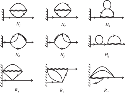
Figure 1: Diagrams contributing to $\Gamma_{0,1}(q,t)_{[\tilde{\phi}_{0}]}$ at two-loop order. Diagrams $H_{1}-H_{6}$ contribute to $\Gamma^{\mathrm{(i)}}_{0,1}(q,t)_{[\tilde{\phi}_{0}]}$; diagrams $R_{1}$,$R_{2}$, and $R_{3}$ contribute to $K(q;t^{\prime},t^{\prime\prime})$. The solid lines correspond to the initial correlator $C^{(i)}_{q}(t,t^{\prime})$ in diagrams $H_{1}-H_{6}$ and to the equilibrium correlator $C^{(e)}_{q}(t,t^{\prime})$ in $R_{1}$,$R_{2}$, and $R_{3}$; the lines with an arrow correspond to the propagator $G_{q}(t,t^{\prime})$; the four-leg vertex $\times$ corresponds to the $g$ interaction; the wavy line corresponds to the disorder interaction $\Delta$; the wall corresponds to the ”time surface” $t=0$.

For $g=\Delta=0$, the generating functional (9) becomes Gaussian and can be easily evaluated in momentum space by solving the corresponding variational equations. We have to take into account the initial condition (8) by imposing the boundary conditions $\tilde{\phi}^{\beta}(\mathbf{x},\infty)=0$ and $\phi_{0}^{\beta}({\bf x})=m_{0}^{\beta}({\bf x})+\tau_{0}^{-1}\tilde{\phi}^{\beta}({\bf x},0)$. The free response function (propagator) $G_{q}(t,t^{\prime})$ and the free correlator $C_{q}(t,t^{\prime})$ are then given by

$$\mbox{}G_{q}(t,t^{\prime})=\Theta(t-t^{\prime})\exp(-\lambda(\tau+\alpha^{2}q_{\parallel}^{2}+q_{\perp}^{2})(t-t^{\prime})),$$ (12)

$$\mbox{}C_{q}(t,t^{\prime})=C_{q}^{(\mathrm{e)}}(t,t^{\prime})+C_{q}^{(\mathrm{i)}}(t,t^{\prime}),$$ (13)

where

$$C_{q}^{(\mathrm{e)}}(t,t^{\prime}) = \frac{\exp(-\lambda(\tau+\alpha^{2}q_{\parallel}^{2}+q_{\perp}^{2})|t-t^{\prime}|)}{\tau+\alpha^{2}q_{\parallel}^{2}+q_{\perp}^{2}},$$ (14)

$$C_{q}^{(\mathrm{i)}}(t,t^{\prime}) = (\tau_{0}^{-1}-\frac{1}{\tau+\alpha^{2}q_{\parallel}^{2}+q_{\perp}^{2}})$$ (15)

$$\times \exp(-\lambda(\tau+\alpha^{2}q_{\parallel}^{2}+q_{\perp}^{2})(t+t^{\prime}))$$

are the equilibrium and the initial nonequilibrium parts of the Gaussian correlator, respectively.

III Renormalization

We now exploit the methods of renormalized field theory in conjunction with a generalized expansion in $\varepsilon$ to investigate the scaling behavior of nonequilibrium response and correlation functions. We define the full one-particle reducible Green functions as

$$G^{\tilde{L}}_{\tilde{N},N}:=\overline{\langle[\phi]^{N}[\tilde{\phi}]^{\tilde{N}}[\tilde{\phi}_{0}]^{\tilde{L}}\rangle}.$$ (16)

The Green functions $G^{\tilde{L}}_{\tilde{N},N}$ may be calculated by a perturbation expansion in the coupling constants $g$ and $\Delta$. The Feynman diagrams that contribute to the Green functions computed using the effective action (11) involve momentum integrations of dimensions $d=4-\varepsilon$ and $\tilde{d}=4-\tilde{\varepsilon}$. We use the dimensional regularizationzinn-justin to calculate integrals and employ the minimal subtraction schemezinn-justin to absorb the remaining poles in $(c_{1}\varepsilon+c_{2}\tilde{\varepsilon})$ into multiplicative Z factors and to introduce the renormalized quantities according to

$$\phi_{b}=Z_{s}^{1/2}\phi,\ \ \tilde{\phi}_{b}=Z_{\tilde{s}}^{1/2}\tilde{\phi},\ \ \tilde{\phi}_{0b}=(Z_{\tilde{s}}Z_{0})^{1/2}\tilde{\phi}_{0},$$

$$\tau_{b}=(Z_{\tau}/Z_{s})\tau,\ \ \ \lambda_{b}=(Z_{s}/Z_{\tilde{s}})^{1/2}\lambda,\ \ \alpha_{b}=Z_{\alpha}\alpha,\ \ \$$ (17)

$$g_{b}=Z_{s}^{-2}Z_{g}g\mu^{\varepsilon},\ \ \Delta_{b}=Z_{s}^{-2}Z_{\Delta}\Delta\mu^{\tilde{\varepsilon}},$$

where the subscript ’b’ denotes bare quantities and $\mu$ is an external momentum scale. Naive dimensional analysis gives $\tau_{0}\propto\mu^{2}$ and, thus, $\tau_{0}^{-1}$ is an irrelevant parameter in the RG sense. It is convenient to consider the Dirichlet boundary conditions $\tau_{0}^{-1}=0$ and $m_{0}^{\beta}(\mathbf{x})=0$. The general case is recovered by treating the parameters $\tau_{0}^{-1}$ and $m_{0}^{\beta}(\mathbf{x})$ as additional perturbations. The Z factors, except for $Z_{0}$, were calculated in Ref. lawrie-84, to two-loop order. The new factor $Z_{0}$ serves to cancel the divergences arising from the initial part $C_{q}^{(\mathrm{i})}(t,t^{\prime})$ for $t+t^{\prime}\to 0$. Note that although there exist two different Z factors for fields $\phi$ and $\tilde{\phi}$, we need only $Z_{0}$ to renormalize fields $\phi_{0}$ and $\tilde{\phi}_{0}$. This is due to the Ward identities

$$\phi^{\beta}_{0}(\mathbf{x})=\tau_{0}^{-1}\tilde{\phi}^{\beta}_{0}(\mathbf{x}),$$ (18)

$$\partial_{t}\phi^{\beta}(\mathbf{x},t)|_{t=0}\equiv\dot{\phi}^{\beta}_{0}(\mathbf{x})=2\lambda\tilde{\phi}^{\beta}_{0}(\mathbf{x}),$$ (19)

which hold when inserted in the connected Green functions.janssen-89 In order to determine $Z_{0}$, we require that

$$(Z_{0}Z_{s}Z_{\tilde{s}})^{-1/2}G^{1}_{0,1}(\mathbf{x},t)=\mathrm{\ finite\ \ for\ }\varepsilon,\ \tilde{\varepsilon}\to 0.$$ (20)

Table 1: Values of two-loop diagrams contributing to $\Gamma_{0,1}(q=0,t)_{[\tilde{\phi}_{0}]}$. The common weight factor for all diagrams is $(n+2)/12(K_{d}g)(K_{\tilde{d}}\Delta)\lambda\Gamma(1-(\varepsilon+\tilde{\varepsilon})/2)(2\lambda t)^{-1+(\varepsilon+\tilde{\varepsilon})/2}$.

$H_{1}$	$-1/\tilde{\varepsilon}-3/4-\varepsilon/4\tilde{\varepsilon}$
$H_{2}$	$1/\tilde{\varepsilon}$
$H_{3}$	$1/\tilde{\varepsilon}-\ln 2/2$
$H_{4}$	$2/\tilde{\varepsilon}+1-2\ln 2$
$H_{5}$	$2/\tilde{\varepsilon}+1+5\ln 2-3\ln 3-\sqrt{3}\ln(2+\sqrt{3})$
$H_{6}$	$-1/\tilde{\varepsilon}+\ln 2/2$
$R_{1}$	$2/\tilde{\varepsilon}$
$R_{2}$	$2\ln 2$
$R_{3}$	$3\ln 3-4\ln 2$

It is more convenient to work with the Fourier transform $G^{1}_{0,1}(q,t)=\int d^{d}x\exp(-{i\mathbf{qx}})G^{1}_{0,1}(\mathbf{x},t)$, which can be written in the following form:

$$G^{1}_{0,1}(q,t)=\int\limits_{0}^{t}dt^{\prime}\bar{G}_{1,1}(q;t,t^{\prime})\Gamma^{\mathrm{(i)}}_{0,1}(q,t^{\prime})_{[\tilde{\phi}_{0}]},$$ (21)

where $\bar{G}_{1,1}(q;t,t^{\prime})$ denotes the full unrenormalized two-point function coming only from the equilibrium part of the correlator (14). $\Gamma^{\mathrm{(i)}}_{0,1}(q,t^{\prime})_{[\tilde{\phi}_{0}]}$ is a reducible one-point vertex function with a single insertion of the response field $\tilde{\phi}_{0}$, which contains in its last irreducible part at least one initial correlator (15). Figure 1 shows the two-loop diagrams $H_{1}$ – $H_{6}$ which contribute to $\Gamma^{\mathrm{(i)}}_{0,1}(q,t^{\prime})_{[\tilde{\phi}_{0}]}$ together with those computed for pure systems in Ref. janssen-89, . The singular parts of computed diagrams are given in Table 1. Note that although $\bar{G}_{1,1}(q;t,t^{\prime})$ is calculated with equilibrium propagators and correlators, it is different from the translational-invariant equilibrium response function $G^{\mathrm{(eq)}}_{1,1}(q;t-t^{\prime})$ because of the restriction of internal time integration to positive times $t\geq 0$. Indeed, the equilibrium Green functions must be calculated by means of the effective action (11) with the lower limit of time integration $t=0$ replaced by $t=-\infty$. We can relate $\bar{G}_{1,1}(q;t,t^{\prime})$ to $G^{\mathrm{(eq)}}_{1,1}(q,t-t^{\prime})$ using the method suggested in Ref. oerding-93, . Following Ref. oerding-93, , we choose the equilibrium distribution $P_{\mathrm{eq}}[\phi_{0}]\propto\exp(-{\cal H}_{V}[\phi_{0}])$ instead of distribution (8) to average over the initial field $\phi_{0}$ in Eq. (9). This allows us to obtain a perturbation series for $G^{\mathrm{(eq)}}_{1,1}(q,t-t^{\prime})$ where internal time integrations range from zero to infinity. However, the non-Gaussian probability distribution $P_{\mathrm{eq}}[\phi_{0}]$ generates in the effective action (11) an additional vertex,

$$- \frac{1}{2}\lambda{\Delta}\int\limits_{0}^{\infty}dt\int d^{d}x\,\int d^{d}x^{\prime}\,\delta^{\tilde{d}}({\mathbf{x}_{\perp}}-{\mathbf{x}_{\perp}^{\prime}})$$ (22)

$$\times \tilde{\phi}^{\beta}(\mathbf{x},t)\phi^{\beta}(\mathbf{x},t)\phi_{0}^{\gamma}(\mathbf{x}^{\prime})\phi_{0}^{\gamma}(\mathbf{x}^{\prime}),$$

which is located at ”time surface” $t=0$. We can relate $G^{\mathrm{(eq)}}_{1,1}(q,t-t^{\prime})$ to $\bar{G}_{1,1}(q;t,t^{\prime})$ by using the following equation:

$$G^{\mathrm{(eq)}}_{1,1}(q,t-t^{\prime})=\int\limits_{t^{\prime}}^{t}dt^{\prime\prime}\bar{G}_{1,1}(q;t,t^{\prime\prime})\Gamma^{\mathrm{(eq)}}_{0,1}(q,t^{\prime\prime})_{[\tilde{\phi}(t^{\prime})]},$$ (23)

where $\Gamma^{\mathrm{(eq)}}_{0,1}(q,t^{\prime\prime})_{[\tilde{\phi}(t^{\prime})]}$ is a reducible vertex function with a single insertion of $\tilde{\phi}(t^{\prime})$, which is calculated with equilibrium correlators and contains in its last irreducible part at least one of the new vertex (22). In contrast to the pure system, janssen-89 the disordered system (1)-(4) has already the nontrivial contributions to $\Gamma^{\mathrm{(eq)}}_{0,1}(q,t^{\prime\prime})_{[\tilde{\phi}(t^{\prime})]}$ at two-loop level. The corresponding two-loop diagrams $R_{1}$ – $R_{3}$ are given in Fig. 1. Considering Eq. (23) as an integral transformation with kernel $\Gamma^{\mathrm{(eq)}}_{0,1}(q,t^{\prime\prime})_{[\tilde{\phi}(t^{\prime})]}$, we can find the kernel of the inverse transformation $K(q;t,t^{\prime})$ order by order in perturbation theory using the following integral equation:

$$\int\limits_{t^{\prime}}^{t}dt^{\prime\prime}\Gamma^{\mathrm{(eq)}}_{0,1}(q,t)_{[\tilde{\phi}(t^{\prime\prime})]}K(q;t^{\prime\prime},t^{\prime})=\delta(t-t^{\prime}).$$ (24)

Combining Eqs. (21), (23), and (24), we arrive at

$$G^{1}_{0,1}(q,t)=\int\limits_{0}^{t}dt^{\prime}G^{\mathrm{(eq)}}_{1,1}(q,t-t^{\prime})\Gamma_{0,1}(q,t^{\prime})_{[\tilde{\phi}_{0}]},$$ (25)

where

$$\Gamma_{0,1}(q,t^{\prime})_{[\tilde{\phi}_{0}]}=\int\limits_{0}^{t^{\prime}}dt^{\prime\prime}K(q;t^{\prime},t^{\prime\prime})\Gamma^{\mathrm{(i)}}_{0,1}(q,t^{\prime\prime})_{[\tilde{\phi}_{0}]}.$$ (26)

The two-loop result for the singular part of vertex function (26) is given by

$$\Gamma_{0,1}(q=0,t)_{[\tilde{\phi}_{0}]}^{\mathrm{sing}} = \delta(t)+\frac{\left(n+2\right)}{12}\lambda g\Gamma\left(1-\,\frac{\varepsilon}{2}\right)\left(2\lambda t\right)^{-1+\varepsilon/2}$$ (27)

$$- \frac{\left(n+2\right)^{2}}{36\varepsilon}\lambda{g}^{2}\Gamma^{2}\left(1-\frac{\varepsilon}{2}\right)\left({\frac{\Gamma^{2}\left(1+\varepsilon/2\right)}{\Gamma\left(1+\varepsilon\right)}}-\frac{1}{2}\right)\left(2\lambda t\right)^{-1+\varepsilon}$$

$$+ \,\frac{\left(n+2\right)}{12}\lambda{g}^{2}\Gamma\left(1-\varepsilon\right)\left(-\frac{1}{\varepsilon}+\ln 2-\frac{1}{2}\right)\left(2\lambda t\right)^{-1+\varepsilon}$$

$$+ \frac{\left(n+2\right)^{2}}{144\varepsilon}\,\lambda{g}^{2}\Gamma^{2}\left(1-\frac{\varepsilon}{2}\right)\left(2\lambda t\right)^{-1+\varepsilon}$$

$$+ \frac{\left(n+2\right)}{48}\lambda g\Delta\Gamma\left(1-\,\frac{\varepsilon+\tilde{\varepsilon}}{2}\right)\left(\frac{24}{\tilde{\varepsilon}}+A-2-\,{\frac{\varepsilon}{\tilde{\varepsilon}}}\right)\left(2\lambda t\right)^{-1+(\varepsilon+\tilde{\varepsilon})/2},$$

where $A=7+4\ln 2-4\sqrt{3}\ln(2+\sqrt{3})$, $\Gamma(x)$ is the Euler gamma function, and we have absorbed factors of $K_{d}=2\pi^{d/2}/((2\pi)^{d}\Gamma(d/2))$ and $K_{\tilde{d}}$ into the redefinition of the coupling constants $g$ and $\Delta$, respectively. Taking into account Eq. (25), the renormalization condition (20) can be rewritten in the form janssen-89 ; oerding-93

$$Z_{0}^{-1/2}\int\limits_{0}^{\infty}dte^{-i\omega t}\Gamma_{0,1}(0,t)_{[\tilde{\phi}_{0}]}^{\mathrm{sing}}=\mathrm{\ finite\ \ for\ }\varepsilon,\ \tilde{\varepsilon}\to 0,$$ (28)

where $\Gamma_{0,1}(0,t)_{[\tilde{\phi}_{0}]}^{\mathrm{sing}}$ is given by Eq. (27) expressed in terms of the renormalized quantities using Eqs. (17). They read in explicit form

$$g\to g_{b}=g\left(1+\frac{(n+8)g}{6\varepsilon}-\frac{6\Delta}{\tilde{\varepsilon}}+O({\varepsilon}^{2},{\varepsilon}\tilde{\varepsilon},\tilde{\varepsilon}^{2})\right),$$

$$\lambda\to\lambda_{b}=\lambda\left(1+\frac{\Delta}{\tilde{\varepsilon}}+O({\varepsilon}^{2},{\varepsilon}\tilde{\varepsilon},\tilde{\varepsilon}^{2})\right).$$

As a result, at two-loop order we obtain

$$Z_{0} = 1+\frac{n+2}{6\varepsilon}g+\frac{n+2}{12\varepsilon^{2}}\left[\frac{n+5}{3}+\left(\ln 2-\frac{1}{2}\right)\varepsilon\right]g^{2}$$ (29)

$$+ \frac{n+2}{24}\frac{(\varepsilon^{2}-24\tilde{\varepsilon}+A\varepsilon\tilde{\varepsilon})}{\varepsilon\tilde{\varepsilon}(\varepsilon+\tilde{\varepsilon})}g\Delta.$$

For $n=1$ and $\tilde{\varepsilon}=\varepsilon$, Hamiltonian (1) corresponds to the Ising model with quenched pointlike disorder, so that Eq. (29) reduces to $Z_{0}$ obtained in Ref. oerding-95, .

IV Scaling and critical exponents

We are now in a position to discuss the scaling properties of Green functions (16). Using the fact that the bare Green function $G^{\tilde{L}}_{\tilde{N},Nb}$ does not depend on the external momentum scale $\mu$ introduced in Eqs. (17), we can derive the RG equation in the usual way. zinn-justin It reads

$$\left[\hat{R}+\frac{N}{2}\gamma+\frac{\tilde{N}}{2}\tilde{\gamma}+\frac{\tilde{L}}{2}(\tilde{\gamma}+\gamma_{0})\right]G^{\tilde{L}}_{\tilde{N},N}=0,$$ (30)

where we have introduced the operator $\hat{R}\equiv\mu{\partial}_{\mu}+\beta_{g}{\partial}_{g}+\beta_{\Delta}{\partial}_{\Delta}+\gamma_{\tau}\tau\partial_{\tau}+\gamma_{\lambda}\lambda\partial_{\lambda}+\gamma_{\alpha}\alpha\partial_{\alpha}$, and the $\beta$ and $\gamma$ functions are defined as derivatives at constant bare parameters,

$$\beta_{g}=\left.\mu{\partial}_{\mu}\ln g\right|_{0},\ \beta_{\Delta}=\left.\mu{\partial}_{\mu}\ln\Delta\right|_{0},\ \gamma_{\alpha}=\left.\mu{\partial}_{\mu}\ln\alpha\right|_{0},\$$

$$\gamma_{\lambda}=\left.\mu{\partial}_{\mu}\ln\lambda\right|_{0}=(\tilde{\gamma}-\gamma)/2,\ \ \ \gamma_{\tau}=\left.\mu{\partial}_{\mu}\ln\tau\right|_{0},$$ (31)

$$\gamma=\left.\mu{\partial}_{\mu}\ln Z_{s}\right|_{0},\ \tilde{\gamma}=\left.\mu{\partial}_{\mu}\ln Z_{\tilde{s}}\right|_{0},\ \gamma_{0}=\left.\mu{\partial}_{\mu}\ln Z_{0}\right|_{0}.\$$

Functions (31), except for $\gamma_{0}$, were calculated in Ref. lawrie-84, to two-loop order. The new function $\gamma_{0}$ reads

$$\gamma_{0}=-\frac{n+2}{6}g\left[1+\left(\ln 2-\frac{1}{2}\right)g+\frac{1}{4}\left(A+\frac{\varepsilon}{\tilde{\varepsilon}}\right)\Delta\right].$$ (32)

The nature of the critical behavior is determined by the existence of a stable fixed point (FP) satisfying the simultaneous equations

$$\beta_{g}(g^{*},\Delta^{*})=0,\ \ \ \beta_{\Delta}(g^{*},\Delta^{*})=0.$$ (33)

The full set of FPs exhibited by Eqs. (33) was discussed in Refs. dorogovtsev-80, and boyanovsky-82, ; prudnikov-83, ; lawrie-84, . We are interested in the FP which controls the critical behavior affected by extended defects. The corresponding FP is given for $n>1$ by lawrie-84

$$g^{*}=\frac{3(3\tilde{\varepsilon}-2\varepsilon)}{2(n-1)}+\frac{3}{256}\left(-4(31n^{2}-68n+196){\varepsilon}^{2}\right.$$

$$+4(73n^{2}+52n+352)\varepsilon\tilde{\varepsilon}-(111n^{2}+696n+624){\tilde{\varepsilon}}^{2}$$

$$\left.-32{(n+2)(n-1){\varepsilon}^{3}}{\tilde{\varepsilon}}^{-1}\right)(n-1)^{-3},$$

$$\Delta^{*}={\frac{(n+8)\tilde{\varepsilon}-2(n+2)\varepsilon}{8(n-1)}}+O({\varepsilon}^{2},{\varepsilon}\tilde{\varepsilon},\tilde{\varepsilon}^{2}).$$ (34)

In the case $n=1$, there is an accidental degeneracy in Eqs. (33), which leads to FPs of order $\varepsilon^{1/2}$ and $\tilde{\varepsilon}^{1/2}$. The FP corresponding to the systems with extended defects reads

$$g^{*}=4\Delta^{*}=8[(9\tilde{\varepsilon}-6\varepsilon)/106]^{1/2}.$$ (35)

The solution of Eq. (30) and the simple dimensional analysis yield the scaling behavior of the Green functions at FPs,

$$\mbox{}G^{\tilde{L}}_{\tilde{N},N}(\{\mathbf{x}_{\parallel},\mathbf{x}_{\perp},t\},\tau,\lambda,\alpha,g^{*},\Delta^{*};\mu)=l^{\varepsilon_{d}(1-\zeta)(N+\tilde{N}+\tilde{L}-2)/2}$$

$$\mbox{}\times l^{(d-2+\eta_{\perp})N/2+(d+2+\tilde{\eta})\tilde{N}/2+(d+2+\eta_{0}+\tilde{\eta})\tilde{L}/2}$$

$$\mbox{}\times G^{\tilde{L}}_{\tilde{N},N}(\{\mathbf{x}_{\parallel}l^{\zeta},\mathbf{x}_{\perp}l,tl^{z_{\perp}}\},\tau l^{-1/\nu_{\perp}},\lambda,\alpha,g^{*},\Delta^{*};\mu),$$ (36)

where the critical exponents are given by

$$\zeta=1-\gamma_{\alpha}(g^{*},\Delta^{*}),\ \ 1/\nu_{\perp}=2-\gamma_{\tau}(g^{*},\Delta^{*}),\$$

$$\eta_{\perp}=\gamma(g^{*},\Delta^{*}),\ \ \ \ \ \ \ z_{\perp}=2+\gamma_{\lambda}(g^{*},\Delta^{*}),\$$ (37)

$$\tilde{\eta}=\tilde{\gamma}(g^{*},\Delta^{*}),\ \ \ \ \ \ \ \ \ \eta_{0}=\gamma_{0}(g^{*},\Delta^{*}).$$

The first factor on the right hand side of Eq. (36) arises from the dependence of Green functions on $\alpha$ not only through $\mathbf{x}_{\parallel}$, but also through an overall factor, which can be easily found out by inspection of the Feynman diagrams (see the Appendix of Ref. lawrie-84, ). Using Eq. (36), we reveal the known relations for the critical exponents, dorogovtsev-80 ; boyanovsky-82 ; prudnikov-83

$$\zeta=\nu_{\parallel}/\nu_{\perp}=(2-\eta_{\perp})/(2-\eta_{\parallel})=z_{\perp}/z_{\parallel}.$$ (38)

Substituting FP (34) into Eq. (32), we obtain the new critical exponent $\eta_{0}$ for $n>1$ as a double expansion in $\varepsilon$ and $\tilde{\varepsilon}$,

$$\eta_{0} = (n+2)(n-1)^{-1}\left[0.5\varepsilon-0.75\tilde{\varepsilon}\right.+(n-1)^{-2}$$ (39)

$$\times \left((0.201599n^{2}+0.601119n+1.992204)\tilde{\varepsilon}^{2}\right.$$

$$- (0.553223n^{2}-0.400168n+3.573508)\tilde{\varepsilon}\varepsilon$$

$$+ (0.284424n^{2}-0.684984n+1.642748)\varepsilon^{2}$$

$$+ \left.\left.(0.03125n^{2}-0.0625+0.03125)\varepsilon^{3}\tilde{\varepsilon}^{-1}\right)\right].$$

In the case $n=1$, we have

$$\eta_{0}=-4[(9\tilde{\varepsilon}-6\varepsilon)/106]^{1/2}.$$ (40)

Note that Eq. (39) involves the ratio $\varepsilon/\tilde{\varepsilon}$, which is of order unity within our approximation. The authors of Ref. prudnikov-83, pointed out that this ratio, which appears in $g^{*}$ and $\gamma_{\tau}$, is absent from the final critical exponents $\nu_{\perp}$, $\eta_{\perp}$, $z_{\perp}$, and $\zeta$ at second order. This encouraged them to believe that similar cancellations will occur at all orders. It is easy to see that the reason for the ratio cancellation is that the last three exponents do not contain the first-order term proportional to $g^{*}$, which gives rise to the ratio $\varepsilon/\tilde{\varepsilon}$ at second order. In the case of $\nu_{\perp}$, the accidental cancellation of terms $\varepsilon/\tilde{\varepsilon}$ occurs when one substitutes FP (34) into $\gamma_{\tau}$. However, the cancellation can be destroyed, for example, by introducing cubic anisotropy, yamazaki-86 so that all exponents involve the ratio $\varepsilon/\tilde{\varepsilon}$. For physical applications, we are interested in positive values $\varepsilon$ and $\tilde{\varepsilon}=\varepsilon+\varepsilon_{d}$, for which $0<\varepsilon/\tilde{\varepsilon}<1$, and therefore the critical exponent (39) is well defined.

In order to describe the scaling behavior of the nonequilibrium critical relaxation, we employ a short-distance expansion of the fields $\phi$ and $\tilde{\phi}$ in terms of the initial fieldsjanssen-89 for $t\to 0$,

$$\phi^{\beta}(t)=\sigma(t)\dot{\phi}_{0}^{\beta}+\ldots,\ \ \ \tilde{\phi}^{\beta}(t)=\tilde{\sigma}(t)\tilde{\phi}_{0}^{\beta}+\ldots.$$ (41)

Introducing the renormalized amplitude functions according to $\sigma_{b}(t)=Z_{0}^{-1/2}\sigma(t)$ and $\tilde{\sigma}_{b}(t)=Z_{0}^{-1/2}\tilde{\sigma}(t)$, we can derive the corresponding RG equations $[\hat{R}-\eta_{0}/2]\sigma(t)=0$ and $[\hat{R}-\eta_{0}/2]\tilde{\sigma}(t)=0$. Taking into account $[\sigma]\sim(\lambda\mu^{2})^{-1}$ and $[\tilde{\sigma}]\sim 1$, we find the solutions of the RG equations at FPs

$$\mbox{}\sigma(t,\tau,\lambda,\alpha;\mu)=l^{-z_{\perp}-\eta_{0}/2}\sigma(tl^{z_{\perp}},\tau l^{-1/\nu_{\perp}},\lambda,\alpha;\mu),$$

$$\mbox{}\tilde{\sigma}(t,\tau,\lambda,\alpha;\mu)=l^{-\eta_{0}/2}\tilde{\sigma}(tl^{z_{\perp}},\tau l^{-1/\nu_{\perp}},\lambda,\alpha;\mu).$$ (42)

We are interested in the short-time critical behavior of the response and correlation functions. Inserting expansions (41) into appropriate Green functions, we obtain $G(\mathbf{x},t,t^{\prime})=\tilde{\sigma}(t^{\prime})G_{0,1}^{1}(\mathbf{x},t)+\ldots$ and $C(\mathbf{x},t,t^{\prime})=2\lambda\sigma(t^{\prime})G_{0,1}^{1}(\mathbf{x},t)+\ldots$, where we have used Eq. (19). Combining Eqs. (36) and (42), we obtain the scaling behavior of the response and correlation functions for $\xi_{\perp}^{-z_{\perp}}t^{\prime}\to 0$ and $\xi_{\perp}^{-z_{\perp}}t>0$,

$$\mbox{}G(\mathbf{x},t,t^{\prime})={x}_{\perp}^{2-d-\eta_{\perp}-z_{\perp}}\left(\frac{t}{t^{\prime}}\right)^{\theta}F_{R}\left(\frac{{x}_{\perp}}{\xi_{\perp}},\frac{{x}_{\perp}}{{x}_{\parallel}^{\zeta}},\frac{t}{\xi_{\perp}^{z_{\perp}}}\right),\ \ \ \$$

$$\mbox{}C(\mathbf{x},t,t^{\prime})={x}_{\perp}^{2-d-\eta_{\perp}}\left(\frac{t}{t^{\prime}}\right)^{\theta-1}F_{C}\left(\frac{{x}_{\perp}}{\xi_{\perp}},\frac{{x}_{\perp}}{{x}_{\parallel}^{\zeta}},\frac{t}{\xi_{\perp}^{z_{\perp}}}\right),\ \ \ \$$ (43)

where the new dynamic critical exponent is defined by

$$\theta=-\eta_{0}/(2z_{\perp}).$$ (44)

To second order in $\varepsilon$ and $\tilde{\varepsilon}$, it reads

$$\theta = (n+2)(n-1)^{-1}\left[0.1875\tilde{\varepsilon}-0.125\varepsilon-(n-1)^{-2}\right.$$ (45)

$$\times \left((0.062119n^{2}+0.232311n+0.404301){\tilde{\varepsilon}}^{2}\right.$$

$$- (0.169556n^{2}-0.021917n+0.784002)\varepsilon\tilde{\varepsilon}$$

$$+ (0.007813n^{2}+0.007813n-0.015625){\varepsilon}^{3}\tilde{\varepsilon}^{-1}$$

$$+ \left.\left.(0.086731n^{2}-0.155621n+0.379437){\varepsilon}^{2}\right)\right].$$

Although the system is characterized by the single exponent $\theta$, the scaling laws (43) reflect the strong anisotropy of the system under consideration.

Table 2: Values of critical exponents $\eta_{0}$, $\theta$, and $\theta^{\prime}$ for $d=3$.

$n$	$\varepsilon_{d}$	$\eta_{0}$	$\theta$	$\theta^{\prime}$
1	0	$-0.374$	$0.092$	$0.087$
	1	$-1.346$	$0.252$	$0.140$
	2	$-1.780$	$0.308$	$0.331$
2	0	$-0.647$	$0.162$ ($0.160$)	$0.200$
	1	$-0.614$	$0.142$ ($0.138$)	$0.059$
	2	$-0.688$	$0.157$ ($0.152$)	$0.054$
3	0	$-0.790$	$0.198$ ($0.196$)	$0.229$
	1	$-0.834$	$0.191$ ($0.186$)	$0.111$
	2	$-1.008$	$0.226$ ($0.214$)	$0.111$

We now discuss the scaling behavior of the order parameter $m^{\beta}(\mathbf{x},t)$ as a function of its initial value $m^{\beta}_{0}(\mathbf{x})$. For the sake of clarity, we will suppress the superscript $\beta$ in what follows. Considering $m_{0}(\mathbf{x})$ as an additional time-independent source coupled to the field $\tilde{\phi}_{0}(\mathbf{x})$, we add the term $\int d^{d}x\,m_{0}(\mathbf{x})\tilde{\phi}_{0}(\mathbf{x})$ to the effective action (11). The order parameter is given then by

$$m(\mathbf{x},t)=\overline{\langle\phi(\mathbf{x},t)\rangle}=\delta W[h,\tilde{h}]/\delta h(\mathbf{x},t)|_{h=\tilde{h}=0}.$$ (46)

Expanding Eq. (46) in $m_{0}$ we obtain for the case of a homogeneous initial order parameter

$$m(m_{0},t)=\sum\limits_{L=1}^{\infty}\frac{1}{L!}\int d^{d}x_{1}\ldots\int d^{d}x_{L}G^{L}_{0,1}(\{\mathbf{x}\},t)m_{0}^{L}.$$ (47)

Equation (47) holds also for the renormalized quantities, so that substituting Eq. (36) into Eq. (47) and summing over $L$, we obtain

$$m(m_{0},t)=m_{0}t^{\theta^{\prime}}F(m_{0}t^{\theta^{\prime}+\beta/\nu_{\perp}z_{\perp}},\tau t^{1/\nu_{\perp}z_{\perp}}),$$ (48)

where $\theta^{\prime}=-[\eta_{\perp}+\tilde{\eta}+\eta_{0}+2\varepsilon_{d}(1-\zeta)]/(2z_{\perp})$, $\beta$ is the critical exponent for the order parameter and we have used the scaling relation $2\beta=\nu_{\perp}(\eta_{\perp}-2+\tilde{d})+\varepsilon_{d}\nu_{\parallel}$. lawrie-84 For $n>1$, we have

$$\theta^{\prime} = 0.125\tilde{\varepsilon}+(n-1)^{-2}$$ (49)

$$\times \left[(0.058228n^{2}-0.062655n+0.204281)\varepsilon\tilde{\varepsilon}\right.$$

$$+ (0.024597n^{2}+0.055126n+0.011862)\varepsilon^{2}$$

$$- (0.007813n^{2}+0.03125n+0.03125)\varepsilon^{3}\tilde{\varepsilon}^{-1}$$

$$- \left.(0.034287n^{2}+0.088644n+0.145612)\tilde{\varepsilon}^{2}\right].$$

The critical exponents $\theta$ and $\theta^{\prime}$ are related by

$$\theta^{\prime}=\theta+(2-\eta_{\perp}-z_{\perp}-\varepsilon_{d}(1-\zeta))/z_{\perp}.$$ (50)

The scaling function $F(y_{1},y_{2})$ has a universal behavior at the critical point $\tau=0$: $F(0,0)$ is finite, while for $y_{1}\to\infty$, $F(y_{1},0)\propto 1/y_{1}$. Thus, Eq. (48) exhibits the crossover between the initial and the equilibrium stages of the critical relaxation at time $t_{c}\propto m_{0}^{-1/(\theta^{\prime}+\beta/\nu_{\perp}z_{\perp})}$, when the initial increasing $m(t)\propto t^{\theta^{\prime}}$ turns to the long-time decreasing $m(t)\propto t^{-\beta/\nu_{\perp}z_{\perp}}$.

It is well known that the convergence of double series in $\varepsilon$ and $\tilde{\varepsilon}$ is poor.lawrie-84 ; blavatska-03 For $n=1$, we know only the lowest order term (40) and cannot apply any resummation technique. Therefore, we compute exponent (40) as it is, and then we calculate $\theta$ and $\theta^{\prime}$ by using Eqs. (44) and (50). In order to estimate the values of the critical exponents $\eta_{0}$, $\theta$, and $\theta^{\prime}$ for $n>1$, we employ the Padé-Borel resummation method extended to the two-parameter case (see Ref. holovatch-02, and references therein). Numerical values of the critical exponents $\eta_{0}$, $\theta$, and $\theta^{\prime}$ computed for the three-dimensional Ising ($n=1$), XY ($n=2$), and Heisenberg ($n=3$) systems with pointlike ($\varepsilon_{d}=0$), linear ($\varepsilon_{d}=1$), and planar ($\varepsilon_{d}=2$) defects are presented in Table 2. To calculate $\theta$ and $\theta^{\prime}$, we can use either expansions (45) and (49), or scaling relations (44) and (50). This can be utilized to check the accuracy of the resummation procedure. The values of $\theta$ given in parenthesis (see Table 2) are computed with the use of Eq. (44). The small discrepancies indicate the fairly good accuracy of the computed values of $\theta$. Unfortunately, using the scaling relation (50) leads to unreasonable values of $\theta^{\prime}$. The reason is the large error in the determination of $\eta_{\perp}$. Indeed, the direct calculation of $\eta_{\perp}$ gives $\eta_{\perp}\approx-0.44$ for $n=2$ and $\varepsilon_{d}=1$,lawrie-84 while the scaling relation $\eta_{\perp}=2-\gamma/\nu_{\perp}$, where $\gamma$ is the critical exponent of susceptibility, suggests $\eta_{\perp}\approx 0.008$. blavatska-03 The resummation of expansion (49) results in more plausible values of $\theta^{\prime}$, which are shown in Table 2.

According to the Harris criterion,harris-74 the pointlike disorder ($\varepsilon_{d}=0$) is relevant for the critical behavior of three-dimensional systems only if $n=1$. The extended defects change the critical behavior for all $n$ if $\varepsilon_{d}>\varepsilon_{d}^{\textrm{marg}}(n)$, where the marginal values $\varepsilon_{d}^{\textrm{marg}}(1)=-0.173$, $\varepsilon_{d}^{\textrm{marg}}(2)=0.016$, and $\varepsilon_{d}^{\textrm{marg}}(3)=0.172$ were calculated for $d=3$ in Ref. blavatska-03, using the extended Harris criterion (5). As one can see from Table 2, the 3D Ising system with extended defects is characterized by larger values of the initial slip exponents $\theta$ and $\theta^{\prime}$ than the 3D Ising system with pointlike disorder. For $n>1$, the pointlike defects do not affect the critical behavior and the critical exponents take the same values as that of the pure system. Table 2 shows that for $n=2,3$, the presence of extended defects leads to the small changes in $\theta$, while the corresponding decrease of $\theta^{\prime}$ is more significant and can be observed in numerical simulations. Remarkably, the decrease of $\theta^{\prime}$ caused by extended defects almost does not depend on $\varepsilon_{d}$ for $n>1$ in the considered approximation.

V Conclusions

In the present paper, we have studied the short-time critical dynamics of the system with extended defects, which are strongly correlated in $\varepsilon_{d}$ dimensions and randomly distributed over the remaining $\tilde{d}=d-\varepsilon_{d}$ dimensions. We have considered the nonequilibrium relaxation of the system starting from a macroscopically prepared initial state with short-range correlations and found the scaling behavior of the nonequilibrium correlation and response functions, and the initial increase of the order parameter. Using the Padé-Borel resummation method, we have calculated the initial slip exponents $\theta$ and $\theta^{\prime}$, which describe the initial growth of correlations, to two-loop order.

Unfortunately, to our knowledge there is only one numerical investigation of the short-time critical dynamics of systems with extended defects. In Ref. zheng-02, , the short-time critical dynamics of the 2D Ising model with bond disorder perfectly correlated in one dimension and uncorrelated in the other was studied using Monte Carlo simulation. This model corresponds to the case $\varepsilon=2$ and $\varepsilon_{d}=1$, for which Eq. (50) gives $\theta^{\prime}=0.154$. The value $\theta^{\prime}=0.176(2)$ reported in Ref. zheng-02, is larger than the prediction of the RG analysis. The difference can be attributed to very strong disorder used in Ref. zheng-02, (the concentration of bonds $p=0.5$), while the RG description is valid only for the regime of weak disorder ($p$ closes to 1), in which the asymptotic behavior does not depend on the concentration $p$.parisi-99

The relevant question is how the critical properties of the system are modified if the defects, oriented along the direction $\mathbf{x}_{\parallel}$, are very long but finite, instead of being extended throughout the system. According to the usual scaling theory near the critical point $T_{c}$, the only relevant scale that remains in the system is the correlation length, which diverges in the critical point as $\xi\propto|\tau|^{-\nu_{p}}$. If the disorder is weak, its effect on the critical behavior in the vicinity of the critical point is negligible as long as the correlation length $\xi$ is smaller than the average distance between the defects $l_{\rm def}$, i.e., the critical behavior is controlled by the FP of the pure system. In close vicinity of the critical point ($\tau\to 0$), the correlation length grows and becomes large than $l_{\rm def}$ for $\tau\ll\Delta^{-1/\varphi}$, where $\varphi$ is the crossover exponent (5). However, it is possible that the correlation length remains smaller than the length of defects. For these values of $\tau$, the critical behavior is controlled by the FP of a system with extended defects, the two correlation lengths naturally arise due to the strong anisotropy, and one can use the results obtained here for the case of the strong correlated disorder. Closer to the critical point, the correlation length $\xi_{\parallel}$ becomes larger than the length of defects and the asymptotic behavior exhibits crossover to the critical behavior of the system with pointlike disorder. The corresponding crossover exponent is $\nu_{\parallel}$.

From an experimental point of view, the considered model may be relevant for the anomalous scaling behavior of the so-called narrow component in magnetic systems such as Ho and Tb, which exhibit two different length scales for critical fluctuations usually ascribed to long-range correlated quenched disorder.altarelli-95 Other possible applications are high-$T_{c}$ superconducting materials, where extended disorder is caused by irregularly alternating layers, such as those containing Y and Ba in Y-Ba-Cu-O structures, or CuO chains. decesare-94 The obtained results can be used to investigate the long-time dynamics of systems with extended defects in the aging regime.calabrese-02 They can be helpful also for numerical simulations of systems with extended defects, especially by using new effective algorithms, based on the fact that due to the small correlation length during the initial stage of the critical relaxation, the determination of critical exponents requires less effort than numerical studies of equilibrium dynamics. li-95

- (1) H.K. Janssen, B. Schaub, and B. Schmittman, Z. Phys. B: Condens. Matter 73, 539 (1989).
- (2) K. Oerding and H.K. Janssen, J. Phys. A 26, 3369 (1993).
- (3) K. Oerding and H.K. Janssen, J. Phys. A 26, 5295 (1993).
- (4) D.A. Huse, Phys. Rev. B 40, 304 (1989); B. Zheng, Int. J. Mod. Phys. B 12, 1419 (1998); B. Zheng, M. Schulz, and S. Trimper, Phys. Rev. Lett. 82, 1891 (1999); H.J. Luo, L. Schülke, and B. Zheng, Phys. Rev. E 64, 036123 (2001).
- (5) Y. Chen, Phys. Rev. B 63, 092301 (2001); Phys. Rev. E 66, 037104 (2002).
- (6) Y. Chen et al., Eur. Phys. J. B 18, 289 (2000).
- (7) J.G. Kissner, Phys. Rev. B 46, 2676 (1992).
- (8) K. Oerding and H.K. Janssen, J. Phys. A 28, 4271 (1995).
- (9) Y. Chen, S.H. Guo, and Z.B. Li, Phys. Status Solidi B 223, 599 (2001).
- (10) P.C. Hohenberg and B.I. Halperin, Rev. Mod. Phys. 49, 435 (1977).
- (11) R.B. Stinchcombe, ”Dilute Magnetism”, in Phase Transitions and Critical Phenomena (Academic Press, London, 1983), Vol. 7.
- (12) J.L. Cardy, Scaling and Renormalization in Statistical Physics (Cambridge University Press, Cambridge, 1996).
- (13) A. Pelissetto and E. Vicari, Phys. Rep. 368, 549 (2002).
- (14) J.J. Alonso and M.A. Muñoz, Europhys. Lett. 56, 485 (2001).
- (15) Yu. Holovatch et al., Int. J. Mod. Phys. B 16, 4027 (2002).
- (16) G. Grinstein and A. Luther, Phys. Rev. B 13, 1329 (1976).
- (17) A.B. Harris, J. Phys. C 7, 1671 (1974).
- (18) A. Weinrib and B.I. Halperin, Phys. Rev. B 27, 413 (1983).
- (19) E. Korutcheva and F. Javier de la Rubia, Phys. Rev. B 58, 5153 (1998).
- (20) V.V. Prudnikov and A.A. Fedorenko, J. Phys. A 32, L399 (1999); V.V. Prudnikov, P.V. Prudnikov, and A.A. Fedorenko, Phys. Rev. B 62, 8777 (2000).
- (21) S.N. Dorogovtsev, Phys. Lett. 76A, 169 (1980); Zh. Eksp. Teor. Fiz 80, 2053 (1981) [Sov. Phys. JETP 53, 1070 (1981)].
- (22) Y. Yamazaki, A. Holz, M. Ochiai, and Y. Fukuda, Physica A 150, 576 (1988).
- (23) D. Boyanovsky and J.L. Cardy, Phys. Rev. B 26, 154 (1982).
- (24) V.V. Prudnikov, J. Phys. C 16, 3685 (1983).
- (25) I.D. Lawrie and V.V. Prudnikov, J. Phys. C 17, 1655 (1984).
- (26) V. Blavats’ka, C. von Ferber, and Yu. Holovatch, Phys. Rev. B 67, 094404 (2003).
- (27) L. De Cesare, Phys. Rev. B 49, 11742 (1994).
- (28) A.L. Korzhenevskii, A.A. Luzhkov, and W. Schirmacher, Phys. Rev. B 50, 3661 (1994).
- (29) Y. Yamazaki, A. Holz, M. Ochiai, and Y. Fukuda, Phys. Rev. B 33, 3460 (1986).
- (30) T. Vojta, J. Phys. A 36, 10921 (2003); R. Sknepnek and T. Vojta, e-print cond-mat/0311394.
- (31) V.S. Dotsenko et al., J. Phys. A 28, 3093 (1995); V.S. Dotsenko and D.E. Feldman, ibid. 28, 5183 (1995).
- (32) G. Tarjus and V. Dotsenko, J. Phys. A 35, 1627 (2002).
- (33) V.V. Prudnikov, P.V. Prudnikov, and A.A. Fedorenko, Phys. Rev. B 63, 184201 (2001); A.A. Fedorenko, J. Phys. A 36, 1239 (2003).
- (34) J. Zinn-Justin, Quantum Field Theory and Critical Phenomena (Clarendon Press, Oxford, 1996).
- (35) J.C. Lee and R.L. Gibbs, Phys. Rev. B 45, 2217 (1992).
- (36) P.C. Martin, E.D. Siggia, and H.A. Rose, Phys. Rev. A 8, 423 (1973).
- (37) C. De Dominicis, Phys. Rev. B 18, 4913 (1978).
- (38) G.P. Zheng and M. Li, Phys. Rev. E 65, 036130 (2002).
- (39) G. Parisi, F. Ricci-Tersenghi, and J.J. Ruiz-Lorenzo, Phys. Rev. E 60, 5198 (1999).
- (40) M. Altarelli, M.D. Núñez-Regueiro, and M. Papoular, Phys. Rev. Lett. 74, 3840 (1995).
- (41) P. Calabrese and A. Gambassi, Phys. Rev. B 66, 212407 (2002).
- (42) Z.B. Li, L. Schülke, and B. Zheng, Phys. Rev. Lett. 74, 3396 (1995).