The dimerized phase of ionic Hubbard models

Abstract

We derive an effective Hamiltonian for the ionic Hubbard model at half filling, extended to include nearest-neighbor repulsion. Using a spin-particle transformation, the effective model is mapped onto simple spin-1 models in two particular cases. Using another spin-particle transformation, a slightly modified model is mapped into an SU(3) antiferromagnetic Heisenberg model whose exact ground state is known to be spontaneously dimerized. From the effective models several properties of the dimerized phase are discussed, like ferroelectricity and fractional charge excitations. Using bosonization and recent developments in the theory of macroscopic polarization, we show that the polarization is proportional to the charge of the elementary excitations.

I Introduction

The ionic Hubbard model (IHM) has been proposed hub ; nag for the description of the neutral-ionic transition in mixed-stack charge-transfer organic crystals tetrathiafulvalene-$p$-chloranil.Lemee ; Horiuchi In the 90’s the interest on the model increased due to its potential application to ferroelectric perovskites.Egami ; res ; ort ; res2 ; gid ; fab ; fab2 ; tor This model is a Hubbard Hamiltonian with nearest-neighbor hopping $t$ and on-site repulsion $U$, on a bipartite lattice with alternating diagonal energy $\pm{\frac{1}{2}}\Delta$ for the two sublattices. At half filling and in the atomic limit ($t\rightarrow 0$), the ground state is a band insulator (BI) for $U<\Delta$ (the sites with diagonal energy $-{\frac{1}{2}}\Delta$ are doubly occupied), but is a Mott insulator (MI) for $U>\Delta$ (all sites singly occupied). The situation is similar to the extended Hubbard model (EHM) with $\Delta=0$ but nearest-neighbor repulsion $V$. tor ; nak ; tsu In the EHM for $t=0$, as $U$ increases, there is a transition from a charge density wave (CDW) insulator, with alternating doubly occupied and empty sites to a MI for $U=2V$. However, while in this model, the result persists for finite small $t$ as it has been shown in second order perturbation theory in $t$,hirsch perturbation theory in the IHM becomes invalid at $U=\Delta$ and non-trivial charge fluctuations persist even in the strong coupling limit. Furthermore while previous results in the IHM were interpreted in terms of only one transition, Fabrizio et al. used arguments based on field theory, which assumes weak coupling (essentially $\Delta\ll U\ll t$), to propose an alternative scenario that includes two transitions as $U$ is increased: the first one is an Ising-like charge transition at $U=U_{c}$ from the BI to a bond-ordered insulator (BOI). When $U$ is further increased, the spin gap vanishes at $U_{s}>U_{c}$ due to a Kosterlitz-Thouless transition between the BOI and the MI.fab ; fab2 An intermediate BOI phase also takes place in the EHM for large enough $t$. nak ; tsu

After the proposal of Fabrizio et al., several studies of the 1D IHM tried to identify the number and the nature of the different phases. Torio et al. determined the phase diagram using the method of crossing of energy levels, which for this model turns out to be equivalent to the method of jumps of Berry phases.tor The basic idea is that while in finite systems conventional order parameters such as charge and spin structure factors vary continuously at a phase transition, in a system of length $L$ one may define charge and spin topological numbers which change discontinuously at $U_{c}(L)$ and $U_{s}(L)$. The charge (spin) Berry phase has a step at $U_{c}(L)$ ($U_{s}(L)$), and extrapolating these numbers to the thermodynamic limits leads usually to accurate results for the transition lines.bos ; topo $U_{c}(L)$ might be detected in transport experiments through some molecules or nanodevices.dots Torio et al. found a phase diagram consistent with the proposal of Fabrizio et al. for weak coupling. They also found that for strong coupling the intermediate BOI phase persists with a width $U_{s}-$ $U_{c}\cong 0.6t$. Recently, similar methods were used to check the characteristics of each quantum phase transition and confirm previous results in systems up to 18 sites.otsu However, Monte Carlo calculations for the bond-order parameter, polarization and localization length were interpreted in terms of only one transition at $U_{c}$ and two phases (BI and BOI).wil In addition, some density-matrix renormalization-group (DMRG) calculations have not detected the transition at $U_{s}$.brune Instead, other DMRG calculations using careful finite-size scaling are consistent with three phases and two transitions and with the phase diagram of Torio et al., although they suggest a smaller width of the BOI phase for small $t$ ($U_{s}-$ $U_{c}\cong 0.4t$).zha ; man

The numerical difficulties for detecting the Kosterlitz-Thouless transition are originated in the exponential closing of the spin gap as $U$ approaches to $U_{s}$ from below. Consequently, direct numerical calculations of the relevant correlation functions are unable to detect a sharp transition at $U_{s}$ unless a very careful finite-size scaling is made. The same difficulty appears in the Hubbard chain with correlated hopping, where the existence and the position of the transition is confirmed by field theory bos ; jap and exact afq results. In the scenario with only one transition there is still a question about the nature of the large $U$ phase ($U>U_{c}$). Wilkens and Martin wil suggested that the MI phase does not exist for finite $t$, i.e., the spin gap remains open for any finite $U$. This is in contradiction with the strong coupling expansion for $t\ll U-\Delta$, which maps the IHM onto an effective spin Hamiltonian $\tilde{H}$ with closed spin gap.nag ; brune ; ali The absence of a spin gap is also supported by the power-law decay of charge-charge correlation functions (in spite of the presence of a charge gap) that have been calculated numerically man and analytically (using $\tilde{H}$),ali with very good agreement between both results. This is a consequence of the strong charge-spin coupling in the low-energy effective theory. These results suggest that if there is only one transition, the BOI phase should disappear from the phase diagram. We mention here that in presence of electron-phonon interaction, the width of the BOI phase increases and, in the adiabatic approximation, it replaces the MI phase.fab ; wil

From the above discussion, it is clear that the existence and extension of the BOI phase in the electronic model deserves further study, particularly in the strong coupling limit, $t\ll U,\Delta$, since the arguments of Fabrizio et al. are not directly applicable. In addition, little attention has been given so far to the electric polarization or ferroelectric properties of the BOI phase.wil ; dimer The BOI phase is an electronically induced Peierls instability that generates a ferroelectric state. Experimentally, a bond ordered ferroelectric state was observed in the pressure-temperature phase diagram of the prototype compound, tetrathiafulvalene-$p$-chloranil Lemee ; Horiuchi . In addition, as it was pointed out by Egami et al., Egami the microscopic origin of the displacive-type ferroelectric transition in covalent perovskite oxides like BaTiO₃ is still unclear. It has been known for a long time that a picture based on static Coulomb interactions and the simple shell model is inadequate to describe some ferroelectric properties.Hippel In a recent paper,dimer using a spin-particle transformation,bat2 ; bat3 we mapped a Hamiltonian which is close to the one obtained in the strong coupling limit of the IHM (in a sense that will become clear in Section IV) into an anisotropic SU(3) antiferromagnetic Heisenberg model that becomes isotropic and exactly solvable in 1D for certain combinations of the parameters. The exact solution is a spontaneously dimerized BOI that helps to understand the physics of the IHM in the strong coupling limit. The large value of the correlation length $\xi=21.0728505...$ allows to understand the numerical difficulties for detecting this phase in finite size systems. We also used a second spin-particle transformation bat1 that maps the constrained fermions into $S=1$ SU(2) spins and brings the effective model into a biquadratic Heisenberg model with a spatial anisotropy along the $z$-axis which is proportional to $\Delta-U$. This allows to interpret both transitions and the fractional charge excitations of the BOI phase in the simple language of $S=1$ spins.

In this work, we derive an effective Hamiltonian $H_{eff}$ for the strong coupling limit of the extended IHM (including $\Delta$ and $V$). As in the $t-J$ model, the single-site Hilbert space of $H_{eff}$ has three states. In two particular relevant cases $H_{eff}$ is mapped into simple models for $S=1$ SU(2) spins. This opens the possibility of studying both quantum phase transitions in 1D with the quantum loop Monte Carlo technique which is specially designed to deal with criticality due to the non-local nature of its dynamics.Jim Harada and Kawashima Kawashima showed that this technique provides an accurate determination of the critical parameters of a Kosterlitz-Thouless transition. The mapping to the exact solution dimer is briefly reviewed. We discuss the polarization of the BOI phase. In particular, we construct the bosonized expressions for the “twist” operators $z_{L}^{c}$ and $z_{L}^{s}$ res2 ; znos ; local which gives information on the conducting and polarization properties of the system, and are also related with the Berry phases. This allows us to relate the polarization in the BOI phase with the charge of its elementary excitations.

II The effective Hamiltonian

In this Section, we derive an effective Hamiltonian for the extended IHM (EIHM) valid for $t\ll\Delta$, but any value of $U$ if $V$ is small.note For simplicity we restrict our study to 1D. The extension of this derivation to dimension higher than one is straightforward but somewhat cumbersome for $V\neq 0$. The Hamiltonian of the EIHM can be written in the form

$$H = -t\sum_{i,\sigma}(f_{i+1\sigma}^{\dagger}f_{i\sigma}^{\;}+{\rm H.c.})+\frac{\Delta}{2}\sum_{i}(-1)^{i}n_{i}$$ (1)

$$+ U\sum_{i}(n_{i\uparrow}-\frac{1}{2})(n_{i\downarrow}-\frac{1}{2})$$

$$+V\sum_{i}(n_{i}-1)(n_{i+1}-1),$$

where $n_{i\sigma}=f_{i\sigma}^{\dagger}f_{i\sigma}^{\;}$, $n_{i}=\sum_{\sigma}n_{i\sigma}$, and $\Delta,t>0$. This Hamiltonian has four states per site: empty, doubly occupied, or singly occupied with spin up or down. At half filling and for $t=0$, all odd sites (those with energy $-\Delta/2$) have at least one particle, and no even site is doubly occupied. Thus, the relevant low-energy Hilbert subspace ${\cal H}_{0}$ has three states per site. Our aim is to eliminate linear terms in $t$ which mix states of ${\cal H}_{0}$ with the rest of the Hilbert space. This can be done with a canonical transformation that leads to an effective Hamiltonian $H_{eff}$ which acts on ${\cal H}_{0}$ and contains terms up to second order in $t$. The procedure is completely standard (see for instance Ref. ali ). To simplify the construction of $H_{eff}$ , it is convenient to perform an electron-hole transformation for the odd sites

$$c_{i\uparrow}^{\dagger} = -f_{i\downarrow}^{\;},\;\;\;c_{i\downarrow}^{\dagger}=f_{i\uparrow}^{\;},\;\;\text{for odd }i$$

$$c_{i\sigma}^{\dagger} = f_{i\sigma}^{\dagger},\;\;\;\;\;\;\;\text{for even }i.$$ (2)

The Hamiltonian now becomes invariant under translation of one site ($i\rightarrow i\pm 1$) but it does not conserve the number of particles due to the particle-hole transformation. The $U(1)$ symmetry associated with the conservation of the total number of electrons is now generated by a the staggered charge operator $Q=\sum_{i,\sigma}(-1)^{i}c_{i\sigma}^{\dagger}c_{i\sigma}^{\;}$. The transformed Hamiltonian becomes

$$H_{2} = -t\sum_{i,\sigma}(c_{i+1\uparrow}^{\dagger}c_{i\downarrow}^{\dagger\;}-c_{i+1\downarrow}^{\dagger\;}c_{i\uparrow}^{\dagger}+\text{H.c.})+\frac{\Delta-U}{2}\sum_{i}n_{i}$$ (3)

$$-V\sum_{i}(n_{i}-1)(n_{i+1}-1)+U\sum_{i}n_{i\uparrow}n_{i\downarrow}.$$

Now, for $t\ll\Delta$ but arbitrary $\Delta-U$,note we can eliminate the states with double occupancy on any site. This constraint can be incorporated to the fermionic algebra by defining the constrained fermion operators:

$${\bar{c}}_{i\sigma}^{\dagger}=c_{i\sigma}^{\dagger}(1-c_{i{\bar{\sigma}}}^{\dagger}c_{i{\bar{\sigma}}}^{\;}),\;\;\;\;\;\;{\bar{c}}_{i\sigma}^{\;}=c_{i\sigma}^{\;}(1-c_{i{\bar{\sigma}}}^{\dagger}c_{i{\bar{\sigma}}}^{\;}).$$ (4)

Performing a canonical transformation we eliminate the terms proportional to $t$. These terms mix the low energy subspace ${\cal H}_{0}$ with the orthogonal high-energy subspace ${\cal H}_{1}$, which consists of all the states having at least one doubly occupied site in this representation. Up to second order in $t$, we obtain the effective Hamiltonian:

$$H_{eff} = -t\sum_{i}({\bar{c}}_{i\uparrow}^{\dagger}{\bar{c}}_{i+1\downarrow}^{\dagger}-{\bar{c}}_{i\downarrow}^{\dagger}{\bar{c}}_{i+1\uparrow}^{\dagger}+\text{H.c.})$$ (5)

$$- V\sum_{i}(1-n_{i})(1-n_{i+1})+E\sum_{i}(n_{i}-1)$$

$$+ \sum_{i}\hat{J}_{i}({\bf s}_{i}\cdot{\bf s}_{i+1}-\frac{1}{4}n_{i}n_{i+1})$$

$$+ \sum_{i\delta=\pm 1}\hat{t}_{i}^{ch}{\bar{c}}_{i+\delta\sigma}^{\dagger}{\bar{c}}_{i-\delta\sigma}(\frac{n_{i}}{2}+2{\bf s}_{i}\cdot{\bf s}_{i-\delta}),$$

where $E=(\Delta-U)/2$, and ${\bf s}_{i}$ is the spin vector at site $i$, the components of which are $s_{i}^{\alpha}=1/2\sum_{\tau,\tau^{\prime}}{\bar{c}}_{i\tau}^{\dagger}\sigma_{\tau\tau^{\prime}}^{\alpha}{\bar{c}}_{i\tau^{\prime}}^{\;}$ with $\alpha=\{x,y,z\}$ ($\sigma^{\nu}$ are the Pauli matrices). The exchange interaction $\hat{J}_{i}$ and correlated hopping $\hat{t}_{i}^{ch}$ coefficients are operators if $V\neq 0$. If $V=0$, $\hat{J}_{i}=2t^{2}/(U+\Delta)$ and $\hat{t}_{i}^{ch}=t^{2}/\Delta$ are constants. $\hat{J}_{i}$ comes from a second order process in which in the original Hamiltonian, the virtual intermediate state has a doubly occupied site at energy $+\Delta/2$ and an empty site at energy $-\Delta/2$. In the original language, $\hat{t}_{i}^{ch}$ represent a correlated hopping between two second nearest-neighbor sites at energy $+\Delta/2$ ($-\Delta/2$) involving an intermediate state with an empty (doubly occupied site) at energy $-\Delta/2$ ($+\Delta/2$).

For general $V$, the expressions of these operators are the following:

$$\hat{J}_{i} = 2t^{2}[\frac{n_{i-1}n_{i+2}}{U+\Delta-V}+\frac{n_{i-1}+n_{i+2}-2n_{i-1}n_{i+2}}{U+\Delta}+$$ (6)

$$+ \frac{(1-n_{i-1})(1-n_{i+2})}{U+\Delta+V}]$$

$$\hat{t}_{i}^{ch} = t^{2}[\frac{1}{\Delta}n_{i-2}n_{i+2}+\frac{1}{\Delta+V}(1-n_{i-2})(1-n_{i+2})$$

$$+ (\frac{1}{\Delta}+\frac{1}{\Delta+V})(n_{i-2}+n_{i+2}-2n_{i-2}n_{i+2})/2].$$

While the general expression of $H_{eff}$ is rather complicated, it takes simpler forms for some particular cases. For instance, if we only keep the linear terms in $t$, what amounts to neglect $\hat{J}_{i}$ and $\hat{t}_{i}^{ch}$, the resulting $H_{eff}^{a}$ already contains the non-trivial charge fluctuations of the EIHM near both transitions and is the minimal model to describe the system in the strong coupling limit. We can rewrite $H_{eff}^{a}$ as a spin 1 model by using the spin-particle transformation bat1

$$S_{j}^{+} = \sqrt{2}\ (\bar{c}_{j\uparrow}^{\dagger}\ K_{j}+K_{j}^{\dagger}\ \bar{c}_{j\downarrow}^{\;}),$$

$$S_{j}^{-} = \sqrt{2}\ (K_{j}^{\dagger}\ \bar{c}_{j\uparrow}^{\;}+\bar{c}_{j\downarrow}^{\dagger}\ K_{j}),$$

$$S_{j}^{z}\ = \bar{n}_{j\uparrow}-\bar{n}_{j\downarrow},$$ (7)

where $K_{j}^{\;}$ is the kink operator bat1 :

$$K_{j}^{\;}=\exp[i\pi\sum_{\begin{subarray}{c}k<j\end{subarray}}\ \bar{n}_{k}]\ .$$ (8)

One way to visualize the effects of this transformation is to note the corresponding mapping of the fermion states at any site to the spin states $|SS^{z}\rangle$: $|j0\rangle\rightarrow|j10\rangle$, ${\bar{c}}_{j\uparrow}^{\dagger}K_{j}^{\;}|0\rangle\rightarrow|j11\rangle$, and ${\bar{c}}_{j\downarrow}^{\dagger}K_{j}^{\;}|0\rangle\rightarrow|j1-1\rangle$. Up to an irrelevant constant, the resulting $H_{eff}$ to first order in $t$ is

$$H_{eff}^{a} = \sum_{i}[t(S_{i}^{x}S_{i+1}^{x}+S_{i}^{y}S_{i+1}^{y})P_{i,i+1}$$ (9)

$$- V(S^{z}_{i})^{2}(S^{z}_{i+1})^{2}\;+(E+2V)(S_{i}^{z})^{2}],$$

where $P_{ij}$ projects over the states with $S_{i}^{z}+S_{j}^{z}=0$ (one may use $P_{ij}=1-(S_{i}^{z}+S_{j}^{z})^{2}$ in Eq. (9) ).

When the second order terms are included for $V=0$ (as in the original IHM), the effective spin Hamiltonian becomes:

$$H_{eff}^{b}=\sum_{i}[t(S_{i}^{x}S_{i+1}^{x}+S_{i}^{y}S_{i+1}^{y})P_{i,i+1}+E(S_{i}^{z})^{2}$$ (10)

$$+ \frac{J}{8}\{(S_{i}^{+}S_{i+1}^{-})^{2}+(S_{i+1}^{+}S_{i}^{-})^{2}+2S_{i}^{z}S_{i+1}^{z}-2(S_{i}^{z})^{2}(S_{i+1}^{z})^{2}\}$$

$$- \frac{t_{ch}}{4}\sum_{\delta=\pm 1}(S_{i+\delta}^{z})^{2}\;(S_{i+\delta}^{x}S_{i-\delta}^{x}+S_{i+\delta}^{y}S_{i-\delta}^{y})(S_{i-\delta}^{z})^{2}$$

$$\times \!\!\!\{(S_{i}^{+}S_{i-\delta}^{-})^{2}+(S_{i-\delta}^{+}S_{i}^{-})^{2}$$

$$+2S_{i}^{z}S_{i-\delta}^{z}+2(S_{i}^{z})^{2}(S_{i-\delta}^{z})^{2}\;\}],$$

where $J=2t^{2}/(U+\Delta)$ and $t_{ch}=t^{2}/\Delta.$

$H_{eff}^{a}$ is the minimal model that describes the physics of the EIHM in the strong coupling limit. It can be studied with quantum Monte Carlo or DMRG and its solution can bring further insight into the nature of the BOI phase, the precise position of the phase transitions, and the effect of $V$ on them. Note that these spin 1 Hamiltonians as well as Eq. (27) below, conserve not only total $S^{z}$, but also the original charge $Q=\sum_{i}(-1)^{i}(S^{z}_{i})^{2}|$, and the ground state is in the $Q=0$ subspace. This seems to be an important reduction of the relevant Hilbert space for numerical calculations.

III Limit of large $V$

For $V\gg t$, the ground state of the EIHM can be obtained by second-order perturbation theory in $t$, extending previous results for the EHM.hirsch One can start either from $H$ or $H_{eff}$. In the latter case, one can easily see that $\hat{t}_{i}^{ch}$ becomes irrelevant and that there is an additional contribution $J_{ad}=2t^{2}/(U-\Delta-V)$ to $J$ when empty sites are eliminated by another canonical transformation.

Starting from a CDW with maximum order parameter, the energy per site up to second order in $t$ becomes

$$E_{II}=-E-V-\frac{t^{2}}{\Delta+3V-U},$$ (11)

where the subscript II means “ionic insulator” to distinguish it from the BI because correlation effects due to $V$ are also present. In the MI phase, one has an effective Heisenberg model with exchange interaction $J_{tot}$ given by Eq.(6) for all $n_{l}=1$ plus $J_{ad}$. From the exact solution, the ground state energy of this model is $-J_{tot}\ln 2$,bah and therefore

$$E_{MI}=-J_{tot}\ln 2\text{; }J_{tot}=\frac{4\Delta t^{2}}{[(U-V)^{2}-\Delta^{2}]}$$ (12)

For $t=0$, the transition between both phases is at $U=\Delta+2V$. At this point, when $V\gg t$, the perturbative corrections in $t^{2}$ converge and the charge fluctuations of both phases have an energy cost $V\gg t$. Consequently, the essential ingredient which can eventually lead to the formation of the BOI phase is absent. Therefore, there are only two phases and one transition in this limit.

IV Bosonization

The previous sections and most of the paper are concerned with the strong-coupling limit, in which $t$ is small compared either to $\Delta$ or the interactions $U,V$. When the interactions are small, usually the continuum limit field theory plus renormalization group allows a precise description of the system.voit ; gog In the EIHM, the usual procedures fail because $\Delta$ is a strongly relevant operator. Nevertheless the bosonized Hamiltonian was used to infer the existence of the intermediate BOI phase in the IHM and the character of its low-energy excitations.fab ; fab2 Here we describe the theory for the EIHM plus exchange interaction to draw conclusions to be used later, and construct the bosonized version of the operators $U_{L}^{c,s}=\exp[i\frac{2\pi}{L}\sum_{j}ja(n_{j\uparrow}\pm n_{j\downarrow})]$, which enter the quantities $z_{L}^{c,s}=\langle g|U_{L}^{c,s}|g\rangle$ where $|g\rangle$ is the ground state, $L$ the length of the system and $a$ the lattice parameter (and short distance cutoff below).

IV.1 Hamiltonian and main results

The bosonized form of $H+J\sum_{i}{\bf s}_{i}\cdot{\bf s}_{i+1}$ is bos ; voit ; schu

$$H=H_{c}+H_{\sigma}+H_{c\sigma},$$ (13)

where $c$ ($\sigma$) denotes charge (spin), $H_{\nu}$ ($\nu=c,\sigma$) is a sine-Gordon Hamiltonian

$$H_{\nu} = \int dx\{\frac{v_{\nu}}{2}[\pi K_{\nu}\Pi_{\nu}^{2}(x)+\frac{(\partial_{x}\phi_{\nu})^{2}}{\pi K_{\nu}}]$$ (14)

$$+\frac{m_{\nu}}{a^{2}}\cos(\sqrt{8}\phi_{\nu})\},$$

and the charge-spin interaction is

$$H_{c\sigma}=\int dx\frac{2\Delta}{\pi a}\cos(\sqrt{2}\phi_{c})\cos(\sqrt{2}\phi_{\sigma}).$$ (15)

In terms of the density operators $\nu_{kr}$ for particles with wave vector $k$ moving in the $r$ (+ or -) direction, the phase fields are schu

$$\phi_{\nu}(x) = -\frac{i\pi}{L}\sum_{k\neq 0}\frac{1}{k}e^{-\eta|k|x-ikx}(\nu_{k+}+\nu_{k-})-\frac{N_{v}\pi x}{L},$$

$$\Pi_{\nu}(x) = \frac{1}{L}\sum_{k\neq 0}e^{-\eta|k|x-ikx}(\nu_{k+}-\nu_{k-})-\frac{J_{v}}{L},$$ (16)

where

$$N_{c,\sigma} = [(N_{+\uparrow}+N_{-\uparrow})\pm(N_{+\uparrow}+N_{-\uparrow})]/\sqrt{2},$$

$$J_{c,\sigma} = [(N_{+\uparrow}-N_{-\uparrow})\pm(N_{+\uparrow}-N_{-\uparrow})]/\sqrt{2},$$ (17)

and $N_{r\sigma}$ is the operator of the total number of particles with spin $\sigma$.

The parameters entering Eqs. (14) are determined by the following equations in terms of the usual g-ology coupling constants:

$$v_{\nu} = \sqrt{(v_{F}^{\nu})^{2}-(\frac{g_{\nu}}{2\pi})^{2}},\;\;\;m_{c}\;=\;\frac{g_{3\perp}}{2\pi^{2}},\;\;\;m_{\sigma}\;=\;\frac{g_{1\perp}}{2\pi^{2}},$$

$$v_{F}^{\rho}\; = \;2ta+\frac{g_{4||}+g_{4\perp}}{\pi},\;\;\;v_{F}^{\sigma}\;=\;2ta+\frac{g_{4||}-g_{4\perp}}{\pi},$$

$$g_{c}\; = \;g_{1||}-2g_{2||}-2g_{2\perp},\;\;\;g_{\sigma}\;=\;g_{1||}-2g_{2||}+2g_{2\perp},$$

$$K_{\nu}\; = \;\sqrt{\frac{2\pi v_{F}^{\nu}+g_{\nu}}{2\pi v_{F}^{\nu}-g_{\nu}}}.$$ (18)

The masses entering Eqs. (14) are proportional to the Umklapp coupling $g_{3\perp}=a(U-2V+3J/2)$ and the backward-scattering one $g_{1\perp}=g_{\sigma}\;=a(U-2V-J/2)$, while $g_{c}<0$ for positive $U$, $V$, and $J$.bos For $\Delta=0$, the charge and spin sectors are decoupled and the usual renormalization group procedure for the sine Gordon model can be applied. By increasing $U$, there is a transition from the II (CDW) to the BOI at $U_{c}=2V-3J/2$, and another one from the BOI to the MI at $U_{s}=2V+J/2$.bos Including second-order corrections to the coupling constants, it has been shown that for $J=0$ the BOI phase still exists for weak $U\sim 2V$.tsu The sign of $g_{3\perp}$ ($g_{1\perp}$) determines the charge (spin) sector. The width of the BOI phase goes to zero with $J$.

For $\Delta\neq 0$, $V=J=0$, Fabrizio et al. fab replaced $H_{c}$ by an effective free massive theory for the MI phase. Then, treating $H_{c\sigma}$ perturbatively, they obtained an effective $H_{\sigma}$ with a renormalized $m_{\sigma}$, showing that lowering $U$, a spin gap opens before the charge transition and therefore a BOI phase exists between the two transitions. They also discussed the excitations of the BOI phase taking the interaction part of the Hamiltonian as a phenomenological Ginzburg-Landau energy functional $F$ with effective interactions. For its importance in what follows we briefly review this analysis. Ignoring some constants and factors and dropping the subscript $\perp$, we can write

$$F = {g}_{3}\alpha_{c}^{2}+{g}_{1}\alpha_{s}^{2}+{\Delta}\alpha_{c}\alpha_{s},$$

$$\alpha_{v} = \cos(\sqrt{2}\phi_{v}).$$ (19)

In Eq. (19) and in the rest of this subsection, the $g_{i}$ and $\Delta$ are effective parameters renormalized by the interactions and their numerical values are different from those given previously. Since we are in the spin sector of the BOI phase, this implies that the spin gap is open and therefore the effective $g_{1}<0$. Then, $|\alpha_{s}|=1$ minimizes the energy. If also $g_{3}<0$ (corresponding to the BI phase) the energy is minimized by either $\alpha_{c}=1$, $\alpha_{s}=-1$ or $\alpha_{c}=-1$, $\alpha_{s}=1$. If one has a soliton (topological excitation) in the system between these two vacua, clearly the jump in both phases is $\Delta\phi_{v}=\pm\pi/\sqrt{2}$. Since the smooth part of the charge $\rho(x)$ (spin $S_{z}(x)$) operator is $-\sqrt{2}\partial_{x}\phi_{c}/\pi$ ($\partial_{x}\phi_{s}/(\sqrt{2}\pi)$) this excitation has total charge 1 and spin 1/2, as expected. If $g_{3}>2\Delta$, the minima occur for $\alpha_{c}=\Delta/(2g_{3})$, $\alpha_{s}=-1$ or $\alpha_{c}=-\Delta/(2g_{3})$, $\alpha_{s}=1$. For an excitation between vacua with different $\alpha_{s}$ the spin is 1/2 as before, but now the smallest change in the charge field is $\Delta\phi_{c}=\pm C_{1/2}(\pi/\sqrt{2})$, being $C_{1/2}=1-2\arccos[\Delta/(2g_{3})]/\pi$ the fractional charge of the excitation. As $g_{3}$ increases, $C_{1/2}$ decreases. This is consistent with a continuous transition to the MI phase, where the elementary excitations are spinons without charge. In addition there is a pure charge excitation between the two possible values of $\phi_{c}$ modulo $2\pi$ for the same values of $\alpha_{c}$ and $\alpha_{s}$. Its charge is $C_{0}=1-C_{1/2}$.

IV.2 The displacement operators

The quantity $z_{L}^{c}=\langle g|U_{L}^{c}|g\rangle$ where $U_{L}^{c}=\exp[i\frac{2\pi}{L}X]$ where $L$ is the length of the system and $X=\sum_{j}ja(n_{j\uparrow}+n_{j\downarrow})]$, was first proposed by Resta and Sorella as an indicator of localization in extended systems.res2 Using symmetry properties, Ortiz and one of us showed that for translationally invariant interacting systems with a rational number $n/m$ of particles per unit cell the correct definition is $\langle g|(U_{L}^{c})^{m}|g\rangle$ znos . This definition was used to characterize metal-insulator and metal-superconducting transitions in one dimensional lattice models. In the thermodynamic limit, $L\rightarrow\infty$, $|z_{L}^{c}|$ is equal to 1 for a metallic periodic system and to 0 for the insulating state. This is also true for non-interacting disordered systems.local In the thermodynamic limit, $z_{L}^{c}$ provides a way to calculate the expectation value of the position operator (related to the macroscopic electric polarization by $P=e\langle X\rangle/L$) and its fluctuations for a periodic system res2 ; znos ; local :

$$\lim_{L\rightarrow\infty}\frac{e}{2\pi m}{\rm Im}\ln z_{L}^{c} = \frac{e}{2\pi m}\gamma_{c}=P-P_{0}\ ,$$

$$-\lim_{L\rightarrow\infty}\frac{L^{2}}{(2\pi m)^{2}}\ln|z_{L}^{c}|^{2} = \langle X^{2}\rangle-\langle X\rangle^{2},$$ (20)

where $\gamma_{c}$ is the charge Berry phase res ; ort ; tor ; topo ; ort2 ; berry and $P_{0}$ some reference polarization. $\gamma_{c}$ is defined modulo $2\pi$ and therefore $P_{0}$ is defined modulo $e/m$. These results were extended to $z_{L}^{s}$, where $X$ is replaced by the difference between the position of up and down operators $\sum_{j}ja(n_{j\uparrow}-n_{j\downarrow})$, $P$ by the corresponding difference in polarization, and $\gamma_{c}$ by the spin Berry phase $\gamma_{s}$.topo ; berry For calculations in finite systems, more accurate results for $\gamma_{v}$ are obtained calculating it directly rather than using the first Eq. (20).znos ; topo However, this expression allows a trivial calculation of $\gamma_{c}$ if all particles in the ground state are localized.topo In particular $\gamma_{c}=0$ for a CDW with maximum order parameter and $\gamma_{c}=\pi$ for a MI with one particle per site. By continuity and considering that $\gamma_{c}$ can only be 0 or $\pi$ modulo $2\pi$ for a system with inversion symmetry and one particle per site, these two values characterize the II and MI phases until the boundary of a phase transition is reached.

The difficulty in finding a bosonized expression for $U_{L}^{c,s}$ is that the exponents are ill defined in a periodic system. Actually this is the reason why $P$ should be defined through the Berry phase or $z_{L}^{c}$.res2 ; znos ; local Nevertheless, as noted earlier,znos $U_{L}^{c}$ is the operator that shifts all one particle momenta by -$2\pi/L$, to the next available wave vector to the left. Then, by inspection of the expressions of the fields Eqs. (16,17), $U_{L}^{c}$ acting on any state increases $N_{-\sigma}$ by one and decreases $N_{+\sigma}$ also by one.note2 Consequently, $U_{L}^{c}$ shifts $\Pi_{c}(x)$ by $-2\sqrt{2}/L$ and leaves the other three fields invariant. From the commutation relation,

$$[\phi_{c}(x),\Pi_{c}(y)]=i\delta(x-y),$$ (21)

it follows that

$$[-i\int dx\phi_{c}(x),\Pi_{c}(y)]=1$$ (22)

Therefore the displacement operator $U_{L}^{c}$ can be constructed as an exponential of the average charge field. A similar analysis can be carried out for $U_{L}^{s}$ and both results can be written as note3

$$U_{L}^{\nu}=\exp(i\sqrt{8}\phi_{\nu}^{a})\text{, }\phi_{\nu}^{a}=\frac{1}{L}\int dx\phi_{\nu}(x).$$ (23)

In the region of parameters such that the interaction $m_{\nu}$ in the sine Gordon model Eq. (14) is relevant according to the renormalization group, $\phi_{\nu}(x)$ gets frozen at the value that minimizes $m_{\nu}\cos(\sqrt{8}\phi_{\nu})$ and the calculation of $U_{L}^{\nu}$ becomes trivial. In particular, for $g_{3\perp}<0$ ($m_{c}<0$ corresponding to a CDW or II) we obtain $\phi_{c}^{a}=\gamma_{c}=0$, while in the MI phase ($U\rightarrow\infty$, $m_{c}>0$) the result is $\sqrt{8}\phi_{c}^{a}=\gamma_{c}=\pi$, in agreement with the values anticipated above.topo The difference in polarization $e/2$ modulo $e$ (see Eq. (20)) is consistent with the transfer of half of the electrons in one lattice parameter which is required to convert a MI into a II in the strong coupling limit.

In the BOI phase, there is a spontaneous breaking of the inversion symmetry in the thermodynamic limit and fractional values of $\gamma_{c}/\pi$ are allowed for $\Delta\neq 0$. The analysis of the previous subsection indicates that in the BOI phase there are two non-equivalent values for the frozen charge field: $\sqrt{2}\phi_{c}^{a}=\pm\arccos[\Delta/(2g_{3})]=\pm\pi C_{0}/2$. Then, using Eqs. (20) and (23) we obtain the following relation between the polarization and the fractional charge of the elementary spinless excitation of the BOI phase:

$$P-P_{0}=\pm\frac{e}{2\pi}\gamma_{c}=\pm\frac{e}{2}C_{0}.$$ (24)

The sign depends on the particular ground state out of the two-fold degenerated manifold which follows from the $Z_{2}$ (spatial inversion) symmetry breaking. If $P_{0}$ is chosen in such a way that $P=0$ for the MI (implying $P_{0}=\pm e/2$), we also obtain:

$$P=\pm\frac{e}{2}C_{1/2}.$$ (25)

V Rigorous results on an approximate effective Hamiltonian

So far, no approximations have been made beyond that of the strong coupling limit. In this Section we describe a simplification of $H_{eff}$ that allows to map it into an exactly solvable model.dimer We neglect the correlated hopping term $t_{ch}$ and treat the exchange term $J$ as an independent parameter. Both approximations are usually applied to the $t-J$ model after its derivation from the Hubbard model in the strong coupling limit esk ; lema in spite of the fact that the correlated hopping term might be important for stabilizing a superconducting resonance-valence-bond ground state.rvb1 ; rvb2

To simplify the expression for the spin Hamiltonian and unveil accidental symmetries that appear for particular combinations of the parameters, it is convenient to change the sign of the $s_{i}^{x}s_{i+1}^{x}$ and $s_{i}^{y}s_{i+1}^{y}$ term in Hamiltonian (5) (this also changes the sign of the term $(S_{i}^{+}S_{i+1}^{-})^{2}+$H.c. in Eq. (10) ) using the gauge transformation

$${\bar{c}}_{i\downarrow}^{\dagger}\rightarrow-{\bar{c}}_{i\downarrow}^{\dagger}\;\;\;\;\text{for}\;\;i=4n\;\;\text{and}\;\;i=4n+1$$

$${\bar{c}}_{i\uparrow}^{\dagger}\rightarrow-{\bar{c}}_{i\uparrow}^{\dagger}\;\;\;\;\text{for}\;\;i=4n+2\;\;\text{and}\;\;i=4n+1.$$ (26)

Then, neglecting $t_{ch}$, adding the term in $V$ in (10), and taking $V=t$, $J=2t$, the spin 1 Hamiltonian takes the SU(2) invariant form:

$$H_{eff}=-t\sum_{i}[\left({\bf S}_{i}\cdot{\bf S}_{i+1}\right)^{2}-1]+E\sum_{i}[(S_{i}^{z})^{2}-1].$$ (27)

For $E=0$, this model has an SU(3) symmetry which is hidden in this representation. The situation is somewhat similar to the supersymmetric $t-J$ model for $J=2t$.pedro ; bares In our case, the SU(3) symmetry is made explicit using a spin-particle transformation described in detail in Ref. dimer For $E=0$, the model is equivalent to an isotropic SU(3) antiferromagnetic Heisenberg model:

$$H_{eff}(E=0)=\sum_{j\in A,\mu,\nu}t{\cal S}^{\mu\nu}(j){\tilde{{\cal S}}}^{\nu\mu}(j+1),$$ (28)

where $A$ is an arbitrary sublattice ($j$ even or odd) in which the three relevant states transform under the fundamental representation ${\cal S}^{\mu\nu}$, while in the other sublattice $B$, the states transform under its conjugate representation ${\tilde{{\cal S}}}^{\nu\mu}$. The Hamiltonian Eq. (28) is invariant under staggered conjugate SU(3) rotations, ${\cal R}$ and ${\cal R}^{\dagger}$, on sublattices $A$ and $B$ respectively and is integrable.Parkinson ; Barber ; Klumper The ground state of the exact solution is spin-dimerized and corresponds to the BOI in the original language. The degree of dimerization can be characterized by the order parameter Xian ; Solyom

$$D=|h_{i-1,i}-h_{i,i+1}|,$$ (29)

where $h_{i-1,i}=|i-1,i\rangle\langle i,i-1|$ is a projector on the SU(3) singlet spin state, $|i-1,i\rangle=\sum_{m}|i-1m\rangle|im\rangle/\sqrt{3}$, at the bond $(i-1,i)$. Note that $3h_{i-1,i}$ coincides with the term with $j=i-1$ in the isotropic SU(3) Heisenberg Hamiltonian Eq. (28). In the original fermion representation, $|i-1,i\rangle$ has the form

$$|i-1,i\rangle=\frac{1}{\sqrt{3}}(f_{k\uparrow}^{\dagger}f_{k\downarrow}^{\dagger}+f_{i-1\uparrow}^{\dagger}f_{i\downarrow}^{\dagger}-f_{i-1\downarrow}^{\dagger}f_{i\uparrow}^{\dagger})|0\rangle,$$ (30)

where $k=i-[1+(-1)^{i}]/2$ is the site of energy $-\Delta/2$ between $i$ and $i+1$. A perfect dimerized state is constructed repeating this SU(3) singlet each two sites. There are two possibilities depending on the initial site chosen, reflecting the Z(2) symmetry breaking of the exact solution. The exact ground state has $D=0.4216D_{0}$ where $D_{0}$ is the value of $D$ for a perfect dimerized state.Xian The value of the gap is rather small ${\tilde{\Delta}=0.173178}t$, and accordingly the correlation length $\xi=21.0728505...$ is very large.Klumper Therefore, one expects that very large systems should be studied to calculate numerically the bond-order parameter or other properties of the BOI.

The significant degree of dimerization and the form of the SU(3) singlets Eq.(30) points out an important degree of covalency in the BOI phase even in the strong coupling limit. This is in contrast to the solutions for the II and MI phases described previously for large $V$ (see Section III).

While the exact solution brings important insight into the physics of a dimerized state, one might wonder if the approximations made in the Hamiltonian, or the parameters chosen, render the results invalid for the IHM. If the IHM is described to first order in $t$, then $t_{ch}$ becomes irrelevant and the question is if the BOI survives after moving $J$ and $V$ from their values at the exact solution to zero. The results presented in Sections II and III, indicate that increasing $V$ tends to close the BOI phase, while increasing $J$ the effect is the opposite. The effect of small changes of $J$, $V$, and $E$ from the exactly solvable point on the energy of the dimer state, can be calculated by first order perturbation theory. In particular, because of the SU(3) symmetry of the ground state, the ground state expectation value of $-({\bf s}_{i}\cdot{\bf s}_{i+1}-n_{i}n_{i+1}/4)$, which is a projector over an SU(2) singlet with two components, is 2/3 times the expectation value of the SU(3) singlet with three components. We can write:

$$\delta E_{BOI} = E_{BOI}-E_{BOI}^{0}=[-\frac{2}{3}(J-2t)$$ (31)

$$-\frac{1}{3}(V-t)]\langle h_{i,i+1}\rangle_{av}+E\langle(S_{i}^{z})^{2}-1\rangle,$$

where $E_{BOI}^{0}$ is the energy at the exactly solvable point and $\langle h_{i,i+1}\rangle_{av}$ is the expectation value $\langle h_{i,i+1}\rangle$ averaged over even and odd $i$. From the energy of the exact solution, we know that Klumper

$$3\langle h_{i,i+1}\rangle_{av}=\langle\left({\bf S}_{i}\cdot{\bf S}_{i+1}\right)^{2}-1\rangle_{av}=1.796863...,$$ (32)

while because of symmetry (all spin 1 projections are equally probable) $\langle(S_{i}^{z})^{2}\rangle=2/3$.

Estimating the energy shifts for the other two phases as in Section II, neglecting terms of order $t^{2}$ we have

$$\delta E_{II} = E_{II}-E_{II}^{0}\simeq E-(V-t)$$

$$\delta E_{MI} = E_{MI}-E_{MI}^{0}\simeq-(J-2t)\ln 2\text{.}$$ (33)

Using these expressions to calculate the energies of the IHM $(V=J=0)$ for small $E$, one obtains that $\delta E_{II}=\delta E_{MI}\cong 1.39t$ when $E/t=1-2\ln 2\cong-0.39$. For this value of $E$, Eq. (31) gives $\delta E_{BOI}\cong 1.13t<\delta E_{II}$. Since we know that $E_{BOI}^{0}<$ $E_{II}^{0}$ and $E_{BOI}^{0}<E_{MI}^{0}$, this implies that the BOI phase is still that of lowest energy in the strong coupling limit of the IHM if $E$ is decreased to $\sim-0.39t$. Numerical results suggest that while this shift in $E$ is in the right direction, its magnitude is nearly two times smaller.tor ; zha ; man

VI Polarization and fractional charge excitations

In this section, we discuss the polarization and fractional charge excitations of the BOI phase. To render the discussion clearer, we begin by calculating these properties in a perfectly dimerized state with the above mentioned SU(3) symmetry. Due to the breaking of Z(2) symmetry, there are two such states as it is shown in Fig.1. Except for a trivial normalization constant, one of them can be written as:

$$|d1\rangle=\prod_{j=0}^{M-1}\Delta_{j}^{\dagger}|0\rangle,$$ (34)

with $\Delta_{j}^{\dagger}=(f_{2j+1\uparrow}^{\dagger}f_{2j+1\downarrow}^{\dagger}+f_{2j\uparrow}^{\dagger}f_{2j+1\downarrow}^{\dagger}-f_{2j\downarrow}^{\dagger}f_{2j+1\uparrow}^{\dagger})$ (the other ground state $|d2\rangle$ is obtained replacing the subscript $2j$ by $2j+2$ in the last two terms). $M=L/(2a)$ is half the number of sites. Using the definitions in Section IV b and applying $U_{L}^{c}$ to our perfectly dimerized ground state $|d1\rangle$ we obtain:

$$\prod_{j=0}^{M-1}e^{i\pi\frac{4j+1}{M}}(e^{\frac{i\pi}{M}}f_{2j+1\uparrow}^{\dagger}f_{2j+1\downarrow}^{\dagger}+f_{2j\uparrow}^{\dagger}f_{2j+1\downarrow}^{\dagger}-f_{2j\downarrow}^{\dagger}f_{2j+1\uparrow}^{\dagger})|0\rangle.$$ (35)

In the thermodynamic limit, $(\exp(i\pi/M)+2)/3\cong\exp(i\pi/3M)$, the mean value of $z_{L}^{c}$ is:

$$z_{L}^{c}(d1)=\langle d1|U_{L}^{c}|d1\rangle\cong e^{i\pi}\prod_{j=0}^{M-1}e^{i\pi/3M}=e^{i\frac{4}{3}\pi}.$$

This result implies a Berry phase equal to $4\pi/3$. Assuming as before that the polarization of the MI phase is zero ($P_{0}=e/2$ modulo $e$) we have for the polarization $P=e/6$, using Eq. (20) with $m=1$. This result has a simple interpretation: the ideal dimer state is composed of isolated “diatomic molecules”and in this case $P$ coincides with the result for one molecule.znos In each molecule, 1/3 of the charge (the weight of the first term in each factor of Eq.(34)) has been displaced from site $2j$ to $2j+1$, and since there is one molecule per two lattice parameters, the dipolar moment has increased by $e/6$.

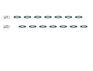
Figure 1: Schematic plot of two dimerized ground states of the BOI.

It is easy to generalize this result out of the SU(3) symmetric point and for the other perfectly dimerized state. The result is (modulo $e$)

$$P(d1)=-P(d2)=\frac{e}{2}\langle n_{1}-1\rangle=\frac{e}{2}\langle 1-(S_{1}^{z})^{2}\rangle\text{.}$$ (36)

The factors that multiply $e/2$ express the weight of doubly occupied sites, i.e., the sites with energy $-\Delta/2$. Note that as $U$ increases these factors decrease and they vanish when the system enters the MI phase. In the opposite limit, at the boundary with the II phase or inside it, there is also only one value of the polarization $P=\pm e/2$ since it is defined modulo $e$. At this point, it is not possible to shift between two different polarized sates by application of an electric field and the system is not ferroelectric. Only inside the BOI phase one has ferroelectricity.

While we are unable to calculate the polarization in the ground state of the BOI phase, our previous result Eq. (25) indicates that the result for the perfectly dimerized states Eq. (36) holds in the general case. The charge of the elementary excitations of the BOI phase can be easily determined in the spin language.dimer Fig. 2 shows a schematic representation of a spinon excitation in which the two possible ground states of the BOI phase are separated by a spin 1 at a given site $i$. This is not an eigenstate because the quantum fluctuations of the spin and the bond ordered regions are not included. However, the inclusion of these fluctuations does not change the charge of the soliton which is connecting both ground states. Since the original charge operator can be written as $Q=\sum_{j}(-1)^{j}|S_{j}^{z}|$, if $S_{i}^{z}=0$ (representing either an empty site or a doubly occupied one), the total change in spin is zero, and the charge of the excitation is $C_{0}=\langle(S_{l}^{z})^{2}\rangle$, where $l$ is any site. If instead $S_{i}^{z}=1$, the spin of the excitation is 1/2 and its charge is $C_{1/2}=\langle 1-(S_{l}^{z})^{2}\rangle$. These results can be related with those of Section IV b and are consistent with Eqs. (25) and (36).

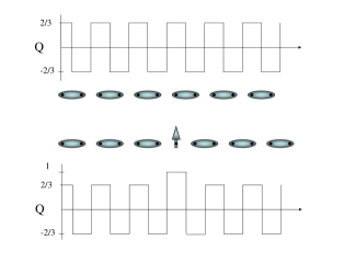
Figure 2: Schematic plot of the soliton excitation of the dimerized ground state in the spin one representation (see Eq. (27) ). In the original fermionic representation, this excitation has spin $S=1/2$ and charge $C_{1/2}=1/3$ at the SU(3) symmetric point.

VII Discussion

In summary, we have derived an effective low energy Hamiltonian for the strong coupling regime of an extended IHM that includes a nearest-neighbor repulsion. Using the spin-particle transformations introduced in Ref. bat1 , we mapped the effective Hamiltonian into a spin one model. The spin language is useful to unveil hidden symmetries of the effective model for particular combinations of the different parameters. For instance, we showed that when the correlated hopping $t_{ch}$ is neglected and the exchange term $J$ is treated as an independent parameter, the effective Hamiltonian becomes a biquadratic Heisenberg model with a single-ion anisotropy for $V=t$ and $J=2t$. In particular, the amplitude of the single-ion anisotropy vanishes in the region dominated by the charge transfer instability: $U=\Delta$. At this point, the Hamiltonian can be rewritten as an SU(3) antiferromagnetic Heisenberg model using the general spin-particle transformations introduced in bat2 ; bat3 . The exact ground state of this model is a dimerized solution that corresponds to the BOI in the original fermionic language. In the spin one language, the low energy excitations of the dimerized solution are spinons. The $S_{z}=0$ spinons carry zero spin and charge $C_{0}=\pm 2/3$ in terms of the original fermions. The $S_{z}=\pm 1$ spinons have spin $s=1/2$ and charge $C_{1/2}=\pm 1/3$ in the original fermionic version. Making $U\neq\Delta$ changes the value of $C_{0}$ and $C_{1}$ continuously as a function of $U-\Delta$ so the charge $Q$ the solitons can also take irrational values.

The above described results, which were obtained in the strong coupling limit, are in qualitative agreement with the weak coupling bosonization approach of Fabrizio et al.fab2 The irrational values of the charge carried by each soliton are just a consequence of the asymmetry between the two sublattices introduced by the $\Delta$ term.Rice Since these excitations have a topological nature, it is expected that their characteristics will not depend on the interaction regime.

In addition, using the bosonization procedure we showed that the polarization of the ferroelectric BOI is proportional to the charge $C_{1/2}$ of the elementary excitations (solitons). Therefore, the magnitude of the fractional charge carried by each soliton can be obtained experimentally by measuring the electric polarization of the ground state.

References

- (1) J. Hubbard and J.B. Torrance, Phys. Rev. Lett. 47, 1750 (1981).
- (2) N. Nagaosa and J. Takimoto, J. Phys. Soc. Jpn. 55, 2735 (1986).
- (3) M. H. Lemée, M. Le Cointe, H. Cailleau, T. Luty, F. Moussa, J. Roos, D. Brinkman, B. Toudic, C. Ayache, and N. Karl, Phys. Rev. Lett. 79, 1690 (1997).
- (4) S. Horiuchi, Y. Okimoto, R. Kumai, and Y. Tokura, J. Phys. Soc. Jpn. 69, 1302 (2000).
- (5) T. Egami, S. Ishihara, and M.Tachiki, Science 261, 1307 (1993); Phys. Rev. B 49, 8944 (1994).
- (6) R. Resta and S. Sorella, Phys. Rev. Lett. 74, 4738 (1995).
- (7) G. Ortiz, P. Ordejón, R.M. Martin, and G. Chiappe, Phys. Rev. B 54, 13 515 (1996); references therein.
- (8) R. Resta and S. Sorella, Phys. Rev. Lett. 82, 370 (1999).
- (9) N. Gidopoulos, S. Sorella, and E. Tosatti, Eur. Phys. J. B 14, 217 (2000).
- (10) M. Fabrizio, A.O. Gogolin, and A.A. Nersesyan, Phys. Rev. Lett 83, 2014 (1999).
- (11) M. Fabrizio, A.O. Gogolin, and A.A. Nersesyan, Nucl. Phys. B 580, 647 (2000).
- (12) M.E. Torio, A.A. Aligia, and H.A. Ceccatto, Phys. Rev. B 64, 121105 (R) (2001).
- (13) M. Nakamura, J. Phys. Soc. Jpn. 68, 3123 (1999); Phys. Rev. B 61, 16 377 (2000).
- (14) M. Tsuchiizu and A. Furusaki, Phys. Rev. Lett 88, 056402 (2002).
- (15) J.E. Hirsch, Phys. Rev. Lett 53, 2327 (1984).
- (16) A.A. Aligia and L. Arrachea, Phys. Rev. B 60, 15 332 (1999) and references therein.
- (17) A.A. Aligia, K. Hallberg, C.D. Batista, and G. Ortiz, Phys. Rev B 61, 7883 (2000).
- (18) A. A. Aligia, K. Hallberg, B. Normand, and A. P. Kampf, Phys. Rev. Lett. 93, 076801 (2004).
- (19) H. Otsuka and M. Nakamura, cond-mat/0403630.
- (20) T. Wilkens and R.M. Martin, Phys. Rev. B 63, 235108 (2001).
- (21) A.P. Kampf, M. Sekania, G.I. Japaridze, and P. Brune, J. Phys. C 15, 5895 (2003).
- (22) Y.Z. Zhang, C.Q. Wu, and H.Q. Lin, Phys. Rev. B 67, 205109 (2003).
- (23) S.R. Manmana, V. Meden, R.M. Noack, and K. Schönhammer, Phys. Rev. B 70, 155115 (2004).
- (24) G.I. Japaridze and A.P. Kampf, Phys. Rev B 59, 12 822 (1999).
- (25) L. Arrachea, A.A. Aligia and E. Gagliano, Phys. Rev. Lett. 76, 4396 (1996); references therein.
- (26) A. A. Aligia, Phys. Rev. B 69, 041101(R) (2004).
- (27) C. D. Batista and A. A. Aligia, Phys. Rev. Lett. 92, 246405 (2004).
- (28) A. R. von Hippel, J. Phys. Soc. Jpn., Supp. 28, 1 (1970).
- (29) C.D. Batista, G. Ortiz and J. Gubernatis , Phys. Rev. B 65, 180402 (2002).
- (30) C.D. Batista and G. Ortiz, Adv. in Phys. 53, 1 (2004).
- (31) C.D. Batista and G. Ortiz, Phys. Rev. Lett. 86, 1082 (2001).
- (32) N. Kawashima, J. E. Gubernatis, and H. G. Evertz, Phys. Rev. B 50, 136 (1994); N. Kawashima, and J. E. Gubernatis, Phys. Rev. Lett. 73, 1295 (1994);
- (33) K.Harada and N. Kawashima, J. Phys. Soc. Jpn. 67, 2768 (1998).
- (34) A.A. Aligia and G. Ortiz, Phys. Rev. Lett. 82, 2560 (1999).
- (35) G. Ortiz and A. A. Aligia, Physica Status Solidi (b) 220, 737 (2000).
- (36) The validity of requires small compared to , , and .
- (37) See for example J. des Cloizeaux and J.J. Pearson, Phys. Rev. 128, 2131 (1962).
- (38) J. Voit, Rep. Prog. in Phys. 58, 977 (1995).
- (39) A.O. Gogolin, A.A. Nersesyan, and A.M. Tsvelick, Bosonization and strongly correlated systems (University Press, Cambridge, 1998).
- (40) H.J. Schulz, Phys. Rev. Lett. 64, 2831 (1990).
- (41) G. Ortiz and R. M. Martin, Phys. Rev. B 49, 14202 (1994).
- (42) We are assuming that the bottom of the band is always filled, as usual in bosonization.
- (43) A similar result for , but with instead of was stated without demostration in M. Nakamura and J. Voit, Phys. Rev. B 65, 153110 (2002).
- (44) A.A. Aligia, Europhys. Lett. 45, 411 (1999).
- (45) H. Eskes, A.M. Oles, M.B.J. Meinders and W. Stephan, Phys. Rev. B 50 17 980 (1994); references therein.
- (46) F. Lema and A.A. Aligia, Phys. Rev. B 55, 14092 (1997); Physica C 307, 307 (1998).
- (47) C. D. Batista and A. A. Aligia, Physica C 264, 319 (1996).
- (48) C. D. Batista, L. O. Manuel, H. A. Ceccatto and A. A. Aligia, Europhys. Lett. 38, 147 (1997).
- (49) P. Schlottmann, Phys. Rev. B 36, 5177 (1987).
- (50) P. A. Bares and G. Blatter, Phys. Rev. Lett. 64, 2567 (1990).
- (51) J. B. Parkinson. J. Phys. C 21, 3793 (1988).
- (52) M. N. Barber and M. T. Batchelor, Phys. Rev. B 40, 4621 (1989).
- (53) A. Klümper, Europhys. Lett. 9, 815 (1989); J. Phys. A 23 809 (1990).
- (54) Y. Xian, Phys. Lett. A 183, 437 (1993).
- (55) G. Fáth and J. Sólyom, Phys. Rev. B 51, 3620 (1995).
- (56) M. J. Rice and E. J. Mele, Phys. Rev. Lett. 49, 1455 (1983).