From Large Scale Rearrangements to Mode Coupling Phenomenology

Abstract

We consider the equilibrium dynamics of Ising spin models with multi-spin interactions on sparse random graphs (Bethe lattices). Such models undergo a mean field glass transition upon increasing the graph connectivity or lowering the temperature. Focusing on the low temperature limit, we identify the large scale rearrangements responsible for the dynamical slowing-down near the transition. We are able to characterize exactly the critical dynamics by analyzing the statistical properties of such rearrangements. We obtain a precise crossover description of the role of activation at the transition. Our approach can be generalized to a large variety of glassy models on sparse random graphs, ranging from satisfiability to kinetically constrained models.

Understanding the slowing down of relaxational dynamics in glass-forming liquids is an important open problem in statistical physics. Two points of view have been developed in the last years. Mode coupling theory (MCT) MCT is based upon a “self-consistent” closure of dynamical equations, and predicts an ergodicity-breaking transition at temperature $T_{\rm d}$. It was later shown that MCT is exact for a class of fully-connected (FC) mean-field models, the dynamical phase transition (DPT) being related to the proliferation of metastable states KiTh ; MCA .

According to an alternative point of view, the dynamical slowing down in supercooled liquids can be traced back to the increasing cooperativity of the dynamics BeGaJPB .

It is a recent discovery that MCT implies diverging correlations as the $T_{\rm d}$ is approached BB . This hints at a possible convergence among the above points of view, and may lead to universal predictions. However, the relation between a diverging correlation length and dynamical slowing-down remains qualitative. This paper aims at filling this gap. By analyzing a particular case, we will show that a detailed picture of the critical dynamics can be obtained through the analysis of highly correlated regions whose size diverges at the transition. Several features of MCT are recovered, despite no exact set of MCT equations holds in the system considered here SeCuMo .

A further source of motivation comes from the discovery that several ensembles of hard optimization problems, such as satisfiability and coloring, undergo a mean-field DPT notrerevue . An interesting question in this context is: how much time a Monte Carlo (MC) algorithm needs for sampling a low-cost configuration of the problem. Furthermore, a phase transition of the same type, is found in a large variety of other models on random graphs, from kinetically constrained models, to rigidity percolation RigidityAndCo .

Finally, there has been a lot of interest in the role of ‘activated processes’ in glasses Kob . In (spherical) FC models free energy barriers vanish above $T_{\rm d}$ while they are extensive (in the system size $N$) below. Activation does not play any role: it is not necessary above $T_{\rm d}$, and it is ineffective below. Schematic MCT does not include activation and is exact for such models, predicting a sharp transition. This picture can be modified in two ways: (A) Requiring barriers to stay finite below $T_{\rm d}$. In finite-dimensional models, this is a consequence of nucleation effects. Activation over such barriers induces a finite time scale for ergodicity restoration, and a smearing of the transition. (B) Introducing finite barriers above $T_{\rm d}$ while keeping extensive ones below. This is the scenario in diluted mean field models, such as the one treated below. While the transition remains sharp, the presence of new (activated) relaxation mechanisms may change the slowing down as $T\downarrow T_{\rm d}$, (e.g. the critical exponents).

In this paper we address the problem (B) above. Since in any realistic (finite-dimensional) model crossing over finite-energy barriers exists at any temperature, it is important to understand if this may modify some key predictions of MCT. In particular, we shall consider a regime in which the distinction between activated and non-activated processes has a precise mathematical sense, i.e. in the neighborhood of a $T=0$ bicritical point.

Our approach is to study a class of large scale rearrangements (LSR) which we expect to control the slow dynamics. Let us begin by providing a loose description of the main ideas on the example of a particle system. Consider a low-$T$  equilibrium configuration and focus on a particular molecule at position $x_{i}$. Now impose a displacement $\delta x_{i}$ (a few intermolecular distances) on this molecule and ask what is the minimum number $n_{i}$ of other molecules which must be moved for this displacement to be possible. The minimum energy barrier $b_{i}$ to be overcome is a second important property of the displacement $\delta x_{i}$. A glassy state is characterized by very large sizes $n_{i}$’s and barriers $b_{i}$’s (diverging at a sharp DPT) leading in turn to large relaxation times. A third quantity is defined by allowing all the molecules within a distance $\ell$ around $x_{i}$ to be moved. Let $\ell_{i}$ be the minimum $\ell$ such that the displacement $\delta x_{i}$ can be performed. It turns out that $n_{i}\ll\ell_{i}^{d}$ (at high enough dimension $d$). Remarkably, molecular dynamics simulations rearr found string-like motions in glass-forming liquids.

Such notions can be completely precised in specific models. In this paper we focus on Ising models with $p$-spin ($p\geq 3$) interactions:

$$H(\sigma)=\frac{1}{2}\sum_{(i_{1}\dots i_{p})\in{\cal G}}(1-J_{i_{1}\dots i_{p}}\sigma_{i_{1}}\cdots\sigma_{i_{p}})\,,$$ (1)

Here $\sigma_{i}=\pm 1$ are $N$ Ising spins, ${\cal G}$ is a set of $M=N\gamma$ $p$-uples of indices, and $J_{i_{1}\dots i_{p}}$ are quenched couplings taking values $\pm 1$ with equal probability. The above Hamiltonian counts the number of violated constraints $\sigma_{i_{1}}\cdots\sigma_{i_{p}}=J_{i_{1}\dots i_{p}}$. This model is known in computer science as XORSAT XOR_CS .

A mean field version of this model is obtained by taking the $M$ interacting $p$-uples of sites $\{(i_{1}\dots i_{p})\}$ to be quenched random variables uniformly distributed in the set of $N\choose p$ possible $p$-uples XOR . In the limit $N\to\infty$, the number of interactions a given spin belongs to (its connectivity) is a Poisson random variable with parameter $p\gamma$. Moreover, the shortest loop through such a spin is (typically) of order $\log_{p\gamma}N$. The phase diagram is sketched in Fig. 1. Two regimes have attracted a particular attention. In the “fully-connected” limit $\gamma\to\infty$, $T\propto\sqrt{\gamma}$, both statics and dynamics can be treated analytically, showing a typical MCT transition. The relaxation time diverges as $|T-T_{\rm d}|^{-\nu}$, while a true thermodynamic transition takes place at $T_{\rm c}$.

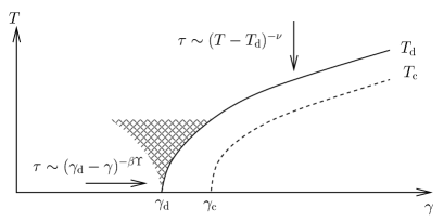
Figure 1: Schematic view of the phase diagram of the diluted $p$-spin model, with its dynamical and static transition line. See the text for details on the two type of divergences encountered at the dynamical transition. The scaling hypothesis of Eq. (3) is expected to hold in the shaded region.

In the $T\downarrow 0$, finite $\gamma$, limit, probabilistic methods can be used to show that zero-energy ground states with finite entropy density exist for $\gamma<\gamma_{\rm c}$. The set of ground states gets splitted in an exponential number of clusters with extensive Hamming distance (number of spins with different value) separating them for $\gamma_{\rm d}<\gamma<\gamma_{\rm c}$ XOR_12 . A finite fraction of the spins does not vary within a particular cluster, while they change when passing from a cluster to the other. At $\gamma_{\rm d}$ the fraction of “frozen” spins jumps from $0$ to a finite value $\phi$. For instance $\gamma_{\rm d}\approx 0.81847$, $\gamma_{\rm c}\approx 0.91793$, and $\phi\approx 0.71533$ when $p=3$. No exact result exists for the dynamics in this regime SeCuMo .

In the region $T<T_{\rm d}(\gamma)$, the Gibbs measure splits into an exponential number of pure states separated by barriers of order $N$. However this implies little (if anything) on the correlation time behavior as $T\downarrow T_{\rm d}(\gamma)$. In agreement with our general philosophy, we shall analyze the dynamics in terms of LSR’s as the transition line $T_{\rm d}(\gamma)$ is approached. The discussion below concerns any single-spin-flip Markov dynamics satisfying detailed balance.

Notice that a diverging length cannot be defined through a standard spin-glass correlation function, which remains short-ranged at $T_{\rm d}(\gamma)$. In order to overcome this problem, consider any temperature $T>T_{\rm d}(\gamma)$ and fix a reference thermalized configuration $\underline{\sigma}^{(0)}$, a site $i$, and a length $\ell$. Denote by $\langle\sigma_{i}\rangle_{\ell}$ the Boltzmann average of $\sigma_{i}$ under the boundary condition $\sigma_{j}=\sigma^{(0)}_{j}$ for any site $j$ at a distance larger than $\ell$ from $i$. Define $\ell_{i}(\varepsilon)$ to be the smallest value of $\ell$ such that $\sigma^{(0)}_{i}\langle\sigma_{i}\rangle\leq\varepsilon$ ($\varepsilon$ being a small fixed number). A standard recursive calculation yields $\ell_{i}(\varepsilon)\sim(T-T_{\rm d}(\gamma))^{-1/2}$ as $T\downarrow T_{\rm d}(\gamma)$. A coupling argument from probability theory can be used OurFuture ; Proba to show that this implies a correlation time $\tau\gtrsim(T-T_{\rm d}(\gamma))^{-1/2}$.

The above argument displays clearly the relation between length and time scales. However the estimate for $\tau$ is not tight (the exponent is incorrect). As we shall see next, a highly refined picture can be obtained as $T\to 0$ in the “liquid” phase $\gamma<\gamma_{\rm d}$. In this regime, the system will spend most of its time in quasi-ground states. For the sake of the argument, assume that it is in fact in a ground state and focus on a particular spin $\sigma_{i}$. The leading mechanism for $\sigma_{i}$ to relax consists in a trajectory in phase space which brings the system to a new ground state with a reversed value of $\sigma_{i}$. Let $F_{i}$ be the set of reversed spins between these two ground states. This set must contain $i$ and, for each interaction $(i_{1}\dots i_{p})\in{\cal G}$, an even number of these $p$ sites. As will be clear from the following, we can restrict in fact to those $F_{i}$’s which are connected, and such that, for each interaction $(i_{1}\dots i_{p})\in{\cal G}$, either two or none of the sites belong to $F_{i}$. In the present context, we call $F_{i}$ a rearrangement for the spin $\sigma_{i}$.

Figure 2: Top: an optimal ordering for this rearrangement $F$. The numbers indicate the energy along the trajectory, here $b(F)=2$. Bottom: example of the recursive construction for $l=3$, $j=2$. Bubbles stand for generic rooted sub-trees. The numbers give the maximal energy in each epoch.

Each $F_{i}$ can be assigned a barrier $b(F_{i})$, defined as the minimum over all (single-spin-flip) paths in configuration space which flip the spins of $F_{i}$, of the maximum energy along the path. Assume that each spin in $F_{i}$ is flipped only once: paths are thus defined by an ordering of the flipped variables. A relaxation time for $\sigma_{i}$ can be defined by considering the correlation function $C_{i}(t)=\langle\sigma_{i}(t)\sigma_{i}(0)\rangle$ and requiring $C_{i}(\tau_{i})=\varepsilon$ for some fixed $\varepsilon$ (in the following $\varepsilon=1/2$). At low temperature, Arrhenius law implies $\tau_{i}\sim\exp[\beta b_{i}]$, with $b_{i}=\min_{F_{i}}b(F_{i})$.

Computing $b_{i}$ requires optimizing both over the choice of the rearrangement $F_{i}$ (the set of spins to be flipped), and over the paths in configuration space (the flipping order). Consider this second task for a given rearrangement $F_{i}$. Form the graph with vertices representing the spins of $F_{i}$, and links between spins belonging to a common interaction in ${\cal G}$. If $F_{i}$ stays finite in the thermodynamic limit, this graph is a tree rooted at $i$. If one draws this tree with vertices placed on an horizontal axis according to the order in which the spins are flipped, the energy of the system at a certain point of the trajectory is simply the number of links drawn above this point, cf. Fig. 2. This ordering problem is studied in graph theory as minimal cutwidth Yanna ; Lengauer .

A simple (and essentially optimal OurFuture ) strategy to construct recursively such an ordering is the following. Assume that the site $i=0$ has $l$ neighbors $\{1\dots l\}\equiv[1,l]$, each one being the root of a sub-tree. Then choose a sequential ordering of the sub-trees, i.e. a permutation $P$ of $[1,l]$, and an integer $j\in[0,l]$. Flip all the variables of the sub-tree $P_{1}$, then do the same on the tree $P_{2}$, and so on until $P_{j}$, then flip the $\sigma_{0}$, and finally flip the spins in the sub-trees $P_{j+1},\dots,P_{l}$. As “proved” in Fig. 2, this construction implies a recursion on the energy barriers

$$b_{0} = \min_{P,j}\max[\;\hat{b}_{P_{1}},1+\hat{b}_{P_{2}},\dots,j-1+\hat{b}_{P_{j}},$$

$$\phantom{\min_{P,j}\max[\;}l-j-1+r+\hat{b}_{P_{j+1}},\dots,r+\hat{b}_{P_{l}}\;]\,,$$

with $r=0$. The $\hat{b}_{i}$’s are “modified barriers” which obey a similar recursion: $\hat{b}_{0}$ is given by Eq. (From Large Scale Rearrangements to Mode Coupling Phenomenology) with $r=1$.

The computation of the barrier $b_{i}$ for the $p$-spin interaction problem still involves an optimal choice of the rearrangement $F_{i}$. This step can also be performed recursively: starting from the root $i$, one chooses in each interaction around it the variable $a$ (among the $p-1$ distinct from $i$) which minimizes $\hat{b}_{a}$. Repeating this step one obtains an admissible rearrangement $F_{i}$ for $\sigma_{i}$, with a minimal value of $b(F_{i})$. Remarkably, this scheme can be efficiently implemented on a given sample OurFuture .

If we consider the ensemble of random hypergraphs ${\cal G}$ described above, the barriers $b_{i}$ become themselves random variables, and Eq. (From Large Scale Rearrangements to Mode Coupling Phenomenology) acquires a distributional meaning. The law $Q_{b}\equiv{\rm Prob}[b_{i}\geq b]$ can be computed numerically and is plotted in Fig. 3 for a few values of $\gamma$ approaching $\gamma_{\rm d}$. Notice that $Q_{b}$ has an immediate physical interpretation in terms of the global correlation function $C(t)=\frac{1}{N}\sum_{i}\langle\sigma_{i}(0)\sigma_{i}(t)\rangle$. At time $t$ only those sites with $b_{i}\gtrsim T\log t$ contribute to the correlation function. We thus have $\lim_{\beta\to\infty}C(e^{\beta(b-\delta)})=Q_{b}$ for any $0<\delta<1$.

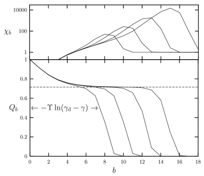
Figure 3: Bottom: integrated law for the distribution of barrier heights. Top: geometrical susceptibility.

The critical behavior of $Q_{b}$ can be solved analytically. As $\gamma$ approaches $\gamma_{\rm d}$ a plateau develops at height $\phi$: a fraction $\phi$ of the spins have “large” barriers (are freezing), while the other ones have “small” barriers. As the plateau is approached (left) one has $Q_{b}\simeq\phi+C_{-}e^{-\omega_{a}b}$ ($Q_{b}\simeq\phi-C_{+}e^{\omega_{b}b}$) with $\omega_{a/b}$ the positive solutions of the equations $2e^{\omega_{a}}-e^{2\omega_{a}}=2e^{-\omega_{b}}-e^{-2\omega_{b}}=\lambda$, and $\lambda$ a $p$-dependent parameter. Finally the scale of the large barriers diverges as $b_{\rm slow}\simeq-\Upsilon\log(\gamma_{\rm d}-\gamma)$, with $\Upsilon=1/(2\omega_{a})+1/(2\omega_{b})$. For instance, if $p=3$ we get $\omega_{a}\approx 0.57432$, $\omega_{b}\approx 1.49574$, and $\Upsilon\approx 1.20488$. The reader will notice the close parallel with the behavior of correlation functions in MCT, with some definite differences: here the divergence is logarithmic rather than power-law; the exponents are no longer fixed by a transcendental relation (see below), but rather through the above quadratic equations for $e^{\omega_{a/b}}$.

Arrhenius law yields a correlation time diverging as $\tau\simeq(\gamma_{\rm d}-\gamma)^{-\beta\Upsilon}$ if the $\gamma\to\gamma_{\rm d}$ limit is taken after $T\to 0$. Inspired by the crossover behavior in diluted ferromagnets Henley , we conjecture the following scaling form to hold if $\gamma\to\gamma_{\rm d}$ together with $T\to 0$:

$$\tau(\beta,\gamma)\simeq e^{\frac{\Upsilon\beta^{2}}{2}}f(e^{\beta}(\gamma-\gamma_{\rm d}))\,.$$ (3)

This summarizes the above findings, as well as the low-$T$ behavior of the dynamic transition line OurFuture : $\gamma_{\rm d}(\beta)\simeq\gamma_{\rm d}+x_{*}e^{-\beta}$ with $x_{*}\approx 9$ for $p=3$. The scaling function behaves as $f(x)\simeq e^{-\Upsilon(\log|x|)^{2}/2}$ as $x\to-\infty$, and $f(x)\simeq f_{+}|x_{*}-x|^{-\nu(\infty)}$ as $x\to x_{*}>0$. In Fig. 4 we check the scaling hypothesis against numerical simulations. Remarkably, Eq. (3) implies a super-Arrhenius behavior at $\gamma_{\rm d}$: $\tau(\beta,\gamma_{\rm d})\propto e^{\Upsilon\beta^{2}/2}$.

Several geometrical properties of optimal (minimum barrier) LSR’s can be determined analytically. Their size (number of sites) diverges as $n_{\rm bar}\sim(\gamma_{\rm d}-\gamma)^{-\nu_{\rm bar}}$, with $\nu_{\rm bar}\approx 2.0157$ for $p=3$. They are non-compact: the chemical distance between the root and a random site in an optimal LSR scales as $(\gamma_{\rm d}-\gamma)^{-\zeta}$, with universal exponent $\zeta=1/2$. Further, optimal rearrangements induce dynamical correlations, as can be understood from the following “experiment”. Consider a site $j\neq i$, and ask what is the minimum barrier $b^{(j)}_{i}$ to be overcome for flipping $\sigma_{i}$ without flipping $\sigma_{j}$. Call $Q^{(j)}_{b}={\rm Prob}[b^{(j)}_{i}\geq b]$, and define the “susceptibility” $\chi_{b}=\sum_{j}[Q^{(j)}_{b}-Q_{b}]$. As $T\to 0$, $\chi_{b}$ describes the change in $C_{i}(t)$ when a pinning field is applied on spin $\sigma_{j}$ (summed over $j$), and is a geometric analogous of the 4-point susceptibility introduced in Chi4 . We show in Fig. 3 its critical behavior. The main feature is a peak located at $b_{\rm peak}\simeq-\Upsilon\log(\gamma_{\rm d}-\gamma)$ whose height $\chi_{\rm peak}\sim(\gamma_{\rm d}-\gamma)^{-\eta}$ (with universal exponent $\eta=1$) estimates the number of spins $\sigma_{j}$ which are influential to the dynamics of $\sigma_{i}$, belonging to all minimal barrier rearrangements for this variable.

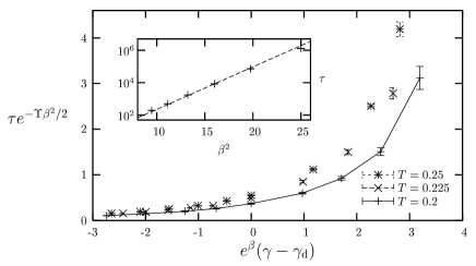
Figure 4: The scaling function of Eq. (3) (notice the large corrections to scaling for $\gamma>\gamma_{\rm d}$). Inset: super-Arrhenius behavior at $\gamma_{d}$.

How does our picture generalize to the $\gamma>\gamma_{\rm d}$, $T\downarrow T_{\rm d}(\gamma)$ regime? Summarizing, we presented two types of results: $(i)$ dynamics proceeds by LSR’s of size $n\sim(\gamma_{\rm d}-\gamma)^{-\nu}$; $(ii)$ the energy barriers to be overcome scales as $b\sim z_{\rm act}\log n$, with $z_{\rm act}=\Upsilon/\nu$. The equilibration time was estimated as $\tau\sim e^{\beta b}\sim n^{\beta z_{\rm act}}$. At finite temperature, the Arrhenius argument does not make sense any more, and one cannot understand slowing down in terms of activated processes. However, we still expect that LSR  sizes diverge as $n\sim(T-T_{\rm d}(\gamma))^{-\nu(\gamma)}$, and that a dynamical scaling relation $\tau\sim n^{z}$ holds with an universal exponent $z$. A partial confirmation is provided by the probabilistic argument discussed in the previous pages implying $\tau\gtrsim(T-T_{\rm d}(\gamma))^{-1/2}$.

How is this related to the issue (B) raised in the introduction? The depth and cooperativity of LSR diverge with two universal exponents $\zeta=1/2$ and $\eta=1$. This agrees with MCT calculations BB implying that such universal features of MCT are not modified by activated processes, even in the regime $e^{-\beta}\ll(\gamma_{\rm d}-\gamma)$. Other features (e.g. the relation $\Gamma(1-a)^{2}/\Gamma(1-2a)=\Gamma(1+b)^{2}/\Gamma(1+2b)$ between $\alpha$- and $\beta$-relaxation exponents) are indeed modified in a crossover region that can be experimentally relevant. However, the asymptotic $T\downarrow T_{\rm d}(\gamma)$ behavior is governed by usual MCT at any $\gamma>\gamma_{\rm d}$. The crossover between the two regimes is ruled by the ratio $(\gamma-\gamma_{\rm d})^{-1}/e^{\beta}$. In a more general context one should consider the ratio $\xi_{\rm dyn}/\xi_{\rm therm}$, where $\xi_{\rm dyn}$ is a dynamical length scale as measured through 4-points correlations BB , and $\xi_{\rm therm}$ is a thermal length (distance between energy defects).

The above ideas can be applied to particle systems. In the particular case of kinetically constrained models on Bethe lattices RigidityAndCo , we could show that the same scenario described above holds OurFuture . A challenging direction would be to analyze ensembles of NP-hard decision problems (random $K$-SAT, or the $q$-coloring of random graphs) with a similar phase diagram SATColoring . Finally, we obtained a purely geometrical description of diverging spatial structures at the DPT. This provides a particularly concrete setting for discussing finite-dimensionality effects.

We thank Leticia Cugliandolo for her interest in this work. G.S. has been partially supported by the EU under the EVERGROW project.

References

- (1) W. Götze, L. Sjögren, Rep. Prog. Phys. 55, 241 (1992).
- (2) T. R. Kirkpatrick and D. Thirumalai, Phys. Rev. B 36, 5388 (1987).
- (3) J.-P. Bouchaud et al., Physica A 226, 243 (1996).
- (4) L. Berthier and J.P. Garrahan, Phys. Rev. E 68, 041201 (2003). J.-P. Bouchaud, cond-mat/0408617.
- (5) G. Biroli and J.-P. Bouchaud, Europhys. Lett. 67 (2004) 21, C. Toninelli, et al. cond-mat/0412158
- (6) G. Semerjian, L. F. Cugliandolo and A. Montanari, J. Stat. Phys. 115, 493 (2004).
- (7) S. Cocco et al., in Computational Complexity and Statistical Physics, A. Percus et al. eds., (Oxford, 2004).
- (8) C. Mourzakel, P. M. Duxbury, and P. L. Leath, Phys. Rev. E 55, 5800 (1997), C. Toninelli, G. Biroli and D. Fisher, Phys. Rev. Lett. 92, 185504 (2004).
- (9) W. Kob, in Slow relaxations and non-equilibrium dynamics in condensed matter, J.-L. Barrat et al. eds. (Springer, Berlin, 2003)
- (10) M. Vogel et al., J. Chem. Phys. 120, 4404 (2004).
- (11) N. Creignou and H. Daudé, Discr. Appl. Math. 96-97 41 (1999).
- (12) F. Ricci-Tersenghi, M. Weigt and R. Zecchina, Phys. Rev. E 63, 026702 (2001).
- (13) M. Mézard, F. Ricci-Tersenghi and R. Zecchina, J. Stat. Phys. 111, 505 (2003). S. Cocco et al. Phys. Rev. Lett. 90, 047205 (2003).
- (14) A. Montanari and G. Semerjian, in preparation.
- (15) N. Berger et al.Prob. Theor. and Rel. Fields, to appear, math.PR/0308284,
- (16) T. Lengauer SIAM J. Alg. Disc. Meth. 3 99, (1982).
- (17) M. Yannakakis Journal of the ACM 32, 950 (1985).
- (18) C.L. Henley, Phys. Rev. Lett. 54, 2030 (1985).
- (19) C. Bennemann et al., Nature, 399, 246 (1999)
- (20) M. Mézard, G. Parisi, and R. Zecchina, Science 297, 812 (2002). R. Mulet et al. Phys. Rev. Lett. 89, 268701 (2002)