Effective magnetic fields in degenerate atomic gases induced by light beams with orbital angular momenta

Abstract

We investigate the influence of two resonant laser beams on the mechanical properties of degenerate atomic gases. The control and probe beams of light are considered to have Orbital Angular Momenta (OAM) and act on the three-level atoms in the Electromagnetically Induced Transparency (EIT) configuration. The theory is based on the explicit analysis of the quantum dynamics of cold atoms coupled with two laser beams. Using the adiabatic approximation, we obtain an effective equation of motion for the atoms driven to the dark state. The equation contains a vector potential type interaction as well as an effective trapping potential. The effective magnetic field is shown to be oriented along the propagation direction of the control and probe beams containing OAM. Its spatial profile can be controlled by choosing proper laser beams. We demonstrate how to generate a constant effective magnetic field, as well as a field exhibiting a radial distance dependence. The resulting effective magnetic field can be concentrated within a region where the effective trapping potential holds the atoms. The estimated magnetic length can be considerably smaller than the size of the atomic cloud.

I Introduction

During the last decade a remarkable progress has been experienced in trapping and cooling atoms. In this respect the creation of atomic Bose-Einstein Condensates (BECs) Davis et al. (1995); Bradley et al. (1995); Dalfovo et al. (1999); Pitaevskii and Stringari (2003) and degenerate Fermi gases DeMarco and Jin (1999); Schreck et al. (2001); Hadzibabic et al. (2003) has been the prime achievement. The atomic BECs and degenerate Fermi gases are systems where an atomic physicist often meets physical phenomena encountered in condensed matter physics. For instance, atoms in optical lattices are often studied using the Hubbard model Jaksch et al. (1998) familiar from solid state physics.

Atoms forming quantum gases are electrically neutral particles and there is no vector potential type coupling of the atoms with a magnetic field. Therefore, a direct analogy between the magnetic properties of degenerate atomic gases and solid state phenomena is not necessarily straightforward. It is possible to produce an effective magnetic field in a cloud of electrically neutral atoms by rotating the system such that the vector potential will appear in the rotating frame of reference Bretin et al. (2004); Schweikhard et al. (2004); Baranov et al. (2005). This would correspond to a situation where the atoms feel a uniform magnetic field. Yet stirring an ultracold cloud of atoms in a controlled manner is a rather demanding task.

There have also been suggestions to take advantage of a discrete periodic structure of an optical lattice to introduce assymetric atomic transitions between the lattice sites Jaksch and Zoller (2003); Mueller (2004); Sørensen et al. (2005). Using this approach one can induce a nonvanishing phase for the atoms moving along a closed path on the lattice, i.e. one can simulate a magnetic flux Jaksch and Zoller (2003); Mueller (2004); Sørensen et al. (2005). However such a way of creating the effective magnetic field is inapplicable to an atomic gas that does not constitute a lattice.

A significant experimental advantage would be gained if a more direct way could be used to induce an effective magnetic field. In a previous letter Juzeliūnas and Öhberg (2004), we have shown how this can be done using two light beams in an Electromagnetically Induced Transparency (EIT) configuration. Here we present a more complete account of the phenomenon. We demonstrate that if at least one of these beams contains an Orbital Angular Momentum (OAM), an effective magnetic field appears, which acts on the electrically neutral atoms. In other words, the coupling between the light and the atoms will provide an effective vector potential in the atomic equations of motion. Compared to the rotating atomic gas, where only a constant effective magnetic field is created Bretin et al. (2004); Schweikhard et al. (2004); Baranov et al. (2005), using optical means will be advantageous since the effective magnetic field can now be shaped by choosing proper control and probe beams. Note that the appearance of our effective vector potential is a manifestation of the Berry connection which is encountered in many different areas of physics Jackiw (1988); Sun and Ge (1990); Dum and Olshanii (1996).

The outline of the paper is as follows. In Sec. II we define a system of three level atoms in the $\Lambda$-configuration and present the equations of motion for the atoms interacting with the control and probe beams of light. In doing this we allow the two beams to have orbital angular momenta along the propagation axis $z$. In Sec. III we derive equations of motion for the center of mass of atoms driven to the dark state. The equations of motion contain the terms due to effective vector and trapping potentials describing an effective magnetic field. In contrast to our previous letter Juzeliūnas and Öhberg (2004), the emerging effective potentials are now fully Hermitian. Yet, the two formulations are shown to give the same effective magnetic field and hence are equivalent. In Secs. IV–V we analyze the effective magnetic field and effective trapping potential in the case where at least one of the light beams contains an orbital angular momentum. We show that the spatial profile of the effective magnetic field can be controlled by applying proper control and probe beams. The concluding Sec. VI summarizes the findings. Finally, Appendix A contains technical details of some of the derivations.

II Formulation

II.1 The system

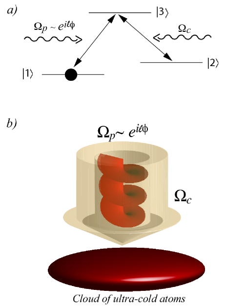
Let us consider a system of atoms characterized by two hyper-fine ground levels $1$ and $2$, as well as an electronic excited level $3$. The atoms interact with two resonant laser beams in the EIT configuration (see Fig. 1b). The first beam (to be referred to as the control beam) drives the transition $|2\rangle\rightarrow|3\rangle$, whereas the second beam (the probe beam) is coupled with the transition $|1\rangle\rightarrow|3\rangle$, see Fig. 1a. The control laser has a frequency $\omega_{c}$, a wave-vector $\mathbf{k}_{c}$, and a Rabi frequency $\Omega_{c}$. The probe field, on the other hand, is characterized by a central frequency $\omega_{p}=ck_{p}$, a wave-vector $\mathbf{k}_{p}$, and a Rabi frequency $\Omega_{p}$. Of special interest is the case where the probe and control beams can carry OAM along the propagation axis $z$. In that case, the spatial distributions of the beams are Allen et al. (1999, 2003)

$$\Omega_{p}=\Omega_{p}^{(0)}e^{i(k_{p}z+l_{p}\phi)}$$ (1)

and

$$\Omega_{c}=\Omega_{c}^{(0)}e^{i(k_{c}z+l_{c}\phi)}\,,$$ (2)

where $\Omega_{p}^{(0)}$ and $\Omega_{c}^{(0)}$ are slowly varying amplitudes for the probe and control fields, $\hbar\ell_{p}$ and $\hbar\ell_{c}$ are the corresponding orbital angular momenta per photon along the propagation axis $z$, and $\phi$ is the azimuthal angle.

Figure 1: (Color online) a) The level scheme for the $\Lambda$ type atoms interacting with the resonant probe beam $\Omega_{p}$ and control beam $\Omega_{c}$. b) Schematic representation of the experimental setup with the two light beams incident on the cloud of atoms. The probe field is of the form $\Omega_{p}\sim e^{i\ell\phi}$, where each probe photon carry an orbital angular momentum $\hbar\ell$ along the propagation axis $z$.

In first quantization, the quantum mechanical state of the atoms is described in terms of the three-component wave function $\Psi_{j}(\mathbf{r},t)$ representing the probability amplitude to find an atom in the $j$-th electronic state and positioned at $\mathbf{r}$, with $j=1,2,3$ . In second quantization, the one-particle wave function $\Psi_{j}(\mathbf{r},t)$ is replaced by the operator $\Psi_{j}(\mathbf{r},t)$ for annihilation of an atom positioned at $\mathbf{r}$ and characterized by an internal state $j$. A set of such operators $\Psi_{j}(\mathbf{r},t)$ obeys the Bose-Einstein or Fermi-Dirac commutation relationships depending on the type of atoms involved. In what follows, $\Psi_{j}(\mathbf{r},t)$ can be understood either as the three-component atomic wave function or as the annihilation field operator. In both cases the spatial and temporal variables will be kept implicit, $\Psi_{j}(\mathbf{r},t)\equiv\Psi_{j}$.

II.2 Initial equations of motion

Introducing the slowly-varying atomic field-operators $\Phi_{1}=\Psi_{1}e^{i\omega_{1}t}$, $\Phi_{3}=\Psi_{3}e^{i(\omega_{1}+\omega_{p})t}$ and $\Phi_{2}=\Psi_{2}e^{i(\omega_{1}+\omega_{p}-\omega_{c})t}$ and adopting the rotating wave approximation, the equations of motion read

$$i\hbar\dot{\Phi}_{1} = -\frac{\hbar^{2}}{2m}\nabla^{2}\Phi_{1}+V_{1}(\mathbf{r})\Phi_{1}+\hbar\Omega_{p}^{*}\Phi_{3}\,,$$ (3)

$$i\hbar\dot{\Phi}_{3} = -\frac{\hbar^{2}}{2m}\nabla^{2}\Phi_{3}+[\epsilon_{31}+V_{3}(\mathbf{r})]\Phi_{3}+\hbar\Omega_{c}\Phi_{2}+\hbar\Omega_{p}\Phi_{1}\,,$$ (4)

$$i\hbar\dot{\Phi}_{2} = -\frac{\hbar^{2}}{2m}\nabla^{2}\Phi_{2}+[\epsilon_{21}+V_{2}(\mathbf{r})]\Phi_{2}+\hbar\Omega_{c}^{*}\Phi_{3}\,,$$ (5)

where $m$ is the atomic mass, $V_{j}(\mathbf{r})$ is the trapping potential for an atom in the electronic state $j$, $\epsilon_{21}=\hbar(\omega_{2}-\omega_{1}+\omega_{c}-\omega_{p})$ and $\epsilon_{31}=\hbar(\omega_{3}-\omega_{1}-\omega_{p})$ are, respectively, the energies of the detuning from the two- and single-photon resonances with $\hbar\omega_{j}$ being the electronic energy of the atomic level $j$.

The equations of motion (3)-(5) do not accommodate collisions between the ground-state atoms. This is a legitimate approximation for a degenerate Fermi gas in which s-wave scattering is forbidden and only weak p-wave scattering is present Butts and Rokhsar (1997); DeMarco and Jin (1999); Mewes et al. (2000); Juzeliūnas and Mašalas (2001). On the other hand, if the atoms in the hyperfine ground states $1$ and $2$ form a BEC, collisions will be present between these atoms. The collisional interaction can however be accommodated if Eqs. (3) and (5) are replaced by the mean-field (Gross-Pitaevskii) equations for the condensate wave-functions,

$$i\hbar\dot{\Phi}_{1} = \left(-\frac{\hbar^{2}}{2m}\nabla^{2}V_{1}(\mathbf{r})+g_{11}|\Phi_{1}|^{2}+g_{12}|\Phi_{2}|^{2}\right)\Phi_{1}+\hbar\Omega_{p}^{*}\Phi_{3}\,,$$ (6)

$$i\hbar\dot{\Phi}_{2} = \left(-\frac{\hbar^{2}}{2m}\nabla^{2}\epsilon_{21}+V_{2}(\mathbf{r})+g_{12}|\Phi_{1}|^{2}+g_{22}|\Phi_{2}|^{2}\right)\Phi_{2}+\hbar\Omega_{c}^{*}\Phi_{3}\,,$$ (7)

where $g_{jl}=4\pi\hbar^{2}a_{jl}/m$, with $a_{jl}$ the s-wave scattering length of the atoms in the electronic states $j$ and $l$, respectively. In particular $a_{jj}$ is the length of the s-wave scattering between a pair of atoms in the same electronic state ($j=1,2$), whereas $a_{12}=a_{21}$ corresponds to collisions between atoms in different electronic states. Since the occupation of the excited atomic level $3$ is small, the atom-atom scattering is of little importance for these atoms and equation (4) for $\Phi_{3}$ can therefore be left unaltered.

III Dark state representation

III.1 Transformed equations of motion

It is convenient to introduce the annihilation field operators for the atoms in the dark and bright states,

$$\Phi_{D} = \frac{1}{\sqrt{1+|\zeta|^{2}}}(\Phi_{1}-\zeta^{*}\Phi_{2})\,,$$ (8)

$$\Phi_{B} = \frac{1}{\sqrt{1+|\zeta|^{2}}}(\zeta\Phi_{1}+\Phi_{2})\,,$$ (9)

where

$$\zeta=\frac{\Omega_{p}}{\Omega_{c}}$$ (10)

is the ratio of the amplitudes of the control and probe fields.

We shall be especially interested in a situation where the atoms are driven to their dark states, described by the creation field operator $\Phi_{D}^{{\dagger}}(\mathbf{r},0)$ acting on the atomic vacuum $|\mathrm{vac}\rangle$. If an atom is in the dark state $|D\rangle\sim|1\rangle-\zeta|2\rangle$, the resonant control and probe beams induce the absorption paths $|2\rangle\rightarrow|3\rangle$ and $|1\rangle\rightarrow|3\rangle$ which interfere destructively, resulting in the Electromagnetically Induced Transparency Arimondo (1996); Harris (1997); Matsko et al. (2001); Lukin (2003). In fact, as one can see from Eq. (4), the transitions to the upper atomic level $3$ are then suppressed, so the atomic level $3$ is weakly populated. This justifies neglection of losses due to spontaneous emissions by the excited atoms in the equation (4) for $\Phi_{3}$.

A transformed set of operators $\Phi_{D}$, $\Phi_{B}$ and $\Phi_{3}$ obeys the following equations of motion (see Appendix A):

$$i\hbar\dot{\Phi}_{D} = \frac{1}{2m}\left(i\hbar\nabla+\mathbf{A}_{\mathrm{eff}}^{(D)}\right)^{2}\Phi_{D}+V_{\mathrm{eff}}^{(D)}(\mathbf{r})\Phi_{D}+F_{DB}(\mathbf{r})\Phi_{B}\,,$$ (11)

$$i\hbar\dot{\Phi}_{B} = \frac{1}{2m}\left(i\hbar\nabla+\mathbf{A}_{\mathrm{eff}}^{(B)}\right)^{2}\Phi_{B}+V_{\mathrm{eff}}^{(B)}(\mathbf{r})\Phi_{B}+\hbar\Omega\Phi_{3}+F_{BD}(\mathbf{r})\Phi_{D}\,,$$ (12)

$$i\hbar\dot{\Phi}_{3} = -\frac{\hbar^{2}}{2m}\nabla^{2}\Phi_{3}+[\epsilon_{31}+V_{3}(\mathbf{r})]\Phi_{3}+\hbar\Omega\Phi_{B}\,,$$ (13)

where

$$\Omega(\mathbf{r})=\sqrt{|\Omega_{p}|^{2}+|\Omega_{c}|^{2}}$$ (14)

is the total Rabi frequency,

$$\mathbf{A}_{\mathrm{eff}}^{(D)}=-\mathbf{A}_{\mathrm{eff}}^{(B)}=\frac{i\hbar}{2}\frac{\zeta^{*}\nabla\zeta-\zeta\nabla\zeta^{*}}{1+|\zeta|^{2}}$$ (15)

is the effective vector potential and

$$V_{\mathrm{eff}}^{(D)}(\mathbf{r}) = \frac{1}{1+|\zeta|^{2}}\left(V_{1}(\mathbf{r})+|\zeta|^{2}(V_{2}(\mathbf{r})+\epsilon_{21})\right)-\frac{i\hbar}{2}\frac{\zeta^{*}\dot{\zeta}-\zeta\dot{\zeta}^{*}}{1+|\zeta|^{2}}$$ (16)

$$+\frac{\hbar^{2}}{2m}\frac{\nabla\zeta^{*}\nabla\zeta}{\left(1+|\zeta|^{2}\right)^{2}}\,,$$

$$V_{\mathrm{eff}}^{(B)}(\mathbf{r}) = \frac{1}{1+|\zeta|^{2}}\left(|\zeta|^{2}V_{1}(\mathbf{r})+V_{2}(\mathbf{r})+\epsilon_{21}\right)-\frac{i\hbar}{2}\frac{\dot{\zeta}^{*}\zeta-\zeta^{*}\dot{\zeta}}{1+|\zeta|^{2}}$$ (17)

$$+\frac{\hbar^{2}}{2m}\frac{\nabla\zeta^{*}\nabla\zeta}{\left(1+|\zeta|^{2}\right)^{2}}$$

are the effective trapping potentials for the atoms in the dark and bright states, respectively. The operators $F_{DB}$ and $F_{BD}$ describing transitions between the dark and bright states in Eqs. (11) and (12), are explicitly defined in Appendix A. Note that the effective vector and trapping potentials $\mathbf{A}_{\mathrm{eff}}^{(D)}$ and $V_{\mathrm{eff}}^{(D)}(\mathbf{r})$ are Hermitian.

The effective magnetic field, corresponding to the effective vector potential $\mathbf{A}_{\mathrm{eff}}^{(D)}$ is

$$\mathbf{B}_{\mathrm{eff}}=\nabla\times\mathbf{A}_{\mathrm{eff}}^{(D)}=i\hbar\frac{1}{\left(1+|\zeta|^{2}\right)^{2}}\nabla\zeta^{*}\times\nabla\zeta\,.$$ (18)

III.2 Equation of motion under adiabatic approximation

In what follows we shall restrict ourselves to the adiabatic case in which transitions between the dark and bright states are not important. In such a situation the term $F_{DB}$ can be neglected in Eq. (11), so it is sufficient to consider a single equation describing the translational motion of the atoms in the dark state:

$$i\hbar\dot{\Phi}_{D}=\frac{1}{2m}\left(i\hbar\nabla+\mathbf{A}_{\mathrm{eff}}^{(D)}\right)^{2}\Phi_{D}+V_{\mathrm{eff}}^{(D)}(\mathbf{r})\Phi_{D}\,.$$ (19)

Assuming that the control and probe fields are tuned to the one- and two-photon resonances ($\epsilon_{31},\epsilon_{21}\ll\hbar\Omega$), the adiabatic approach holds if the matrix elements of the operators $F_{DB}$ and $F_{BD}$ are much smaller than the total Rabi frequency $\Omega$. This leads to the following requirement for the velocity-dependent term in $F_{DB}$

$$F\ll\Omega\,.$$ (20)

Here the velocity-dependent term

$$F=\frac{1}{1+|\zeta|^{2}}\left|\nabla\zeta\cdot\mathbf{v}\right|$$ (21)

reflects the two-photon Doppler detuning. Note that the estimation (20) does not accommodate effects due to the decay of the excited atoms. The dissipation effects can be included replacing the energy of the one-photon detuning $\epsilon_{31}$ by $\epsilon_{31}-i\hbar\gamma_{3}$, where $\gamma_{3}$ is the excited-state decay rate. In such a situation, the dark state can be shown to acquire a finite lifetime

$$\tau_{D}\sim\gamma_{3}^{-1}\Omega^{2}/F^{2}$$ (22)

which should be large compared to other characteristic times of the system. The adiabatic conditions will be further analyzed in Subsection IV.3.

If the atoms in the hyperfine ground states $1$ and $2$ form a BEC, the atomic dynamics in these states is governed by the mean field equations (6)-(7). In such a situation, the equation of motion for the dark state atoms modifies as

$$i\hbar\dot{\Phi}_{D}=\frac{1}{2m}\left(i\hbar\nabla+\mathbf{A}_{\mathrm{eff}}^{(D)}\right)^{2}\Phi_{D}+V_{\mathrm{eff}}^{(D)}(\mathbf{r})\Phi_{D}+g_{D}|\Phi_{D}|^{2}\Phi_{D}\,,$$ (23)

where

$$g_{D}=\frac{1}{\left(1+|\zeta|^{2}\right)^{2}}(g_{11}+2g_{12}|\zeta|^{2}+|\zeta|^{4}g_{22})$$ (24)

describes the interaction between the atoms in the dark state.

III.3 Relation to previous work

In our previous letter Juzeliūnas and Öhberg (2004) an effective equation of motion has been derived for the atoms in the hyperfine ground level $1$. In doing this, the atoms were assumed to be driven to their dark states by imposing the constraint $\Phi_{2}(\mathbf{r},t)=-\zeta\Phi_{1}(\mathbf{r},t)$, which is equivalent to the requirement $\Phi_{B}(\mathbf{r},t)=0$. The resulting effective equation of motion for $\Phi_{1}(\mathbf{r},t)$ reads Juzeliūnas and Öhberg (2004):

$$i\hbar\dot{\Phi}_{1}=\frac{1}{2m}\left[i\hbar\nabla+\mathbf{A}_{\mathrm{eff}}\right]^{2}\Phi_{1}+V_{\mathrm{eff}}(\mathbf{r})\Phi_{1}\,,$$ (25)

where the effective vector and trapping potentials are generally non-Hermitian. For instance, the effective vector potential featured in Eq. (25) is given by Juzeliūnas and Öhberg (2004):

$$\mathbf{A}_{\mathrm{eff}}=\frac{i\hbar\zeta^{*}\nabla\zeta}{1+|\zeta|^{2}}\equiv\mathbf{A}_{\mathrm{eff}}^{(D)}-i\hbar\nabla\ln\left(1+|\zeta|^{2}\right)^{-1/2}\,.$$ (26)

Non-Hermitian potentials appear because the atoms in the electronic state $1$ constitute an open sub-system. In fact, the probe and control beams transfer reversibly atomic population from level $1$ to level $2$ by means of the two-photon Raman transition.

Using the constraint $\Phi_{2}=-\zeta\Phi_{1}$, one can express the dark-state operator $\Phi_{D}$ given by Eq. (8) in terms of $\Phi_{1}$ as:

$$\Phi_{D}=\Phi_{1}\left(1+|\zeta|^{2}\right)^{1/2}\equiv\Phi_{1}\exp\left[\ln\left(1+|\zeta|^{2}\right)^{1/2}\right]\,.$$ (27)

Equation (27) represents a pseudo-gauge (non-unitary) transformation relating the effective equation of motion (25) for $\Phi_{1}$ to the corresponding equation for the dark-state operator $\Phi_{D}$. The transformation (27) is not unitary as long as the intensity of the probe field is non-zero ($|\zeta|\neq 0$). The transition from the unitary equation of motion for $\Phi_{D}$ to the non-unitary one for $\Phi_{1}$ is accompanied by of the non-Hermitian vector and trapping potentials $\mathbf{A}_{\mathrm{eff}}$ and $V_{\mathrm{eff}}$. The Hermitian potential $\mathbf{A}_{\mathrm{eff}}^{(D)}$ differs from its non-Hermitian counterpart $\mathbf{A}_{\mathrm{eff}}$ by a gradient of the imaginary function $i\hbar\ln(1+|\zeta|^{2})^{-1/2}$, as one can see from Eq. (25). In a similar manner, the Hermitian trapping potential $V_{\mathrm{eff}}^{(D)}(\mathbf{r})$ can be shown to differ from the non-Hermitian potential $V_{\mathrm{eff}}(\mathbf{r})$ by the time-derivative of the imaginary function $-i\hbar\ln(1+|\zeta|^{2})^{-1/2}$. In this way the two formulations are equivalent. Since $\mathbf{A}_{\mathrm{eff}}^{(D)}$ differs from $\mathbf{A}_{\mathrm{eff}}$ by a gradient, the effective magnetic field [Eq. (18)] acting on the dark-state atoms, is the same in both formulations.

IV Effective potentials due to light beams with OAM

IV.1 Representation in terms of the amplitude and phase

Separating the ratio $\zeta$ into an amplitude and phase,

$$\zeta=\Omega_{p}/\Omega_{c}=|\zeta|e^{iS}\,,$$ (28)

the effective vector and trapping potentials given by Eqs. (15) and (16) can be rewritten as

$$\mathbf{A}_{\mathrm{eff}}^{(D)}=-\hbar\frac{|\zeta|^{2}}{1+|\zeta|^{2}}\nabla S$$ (29)

and

$$V_{\mathrm{eff}}^{(D)}(\mathbf{r})=V_{\mathrm{ext}}(\mathbf{r})+\frac{\hbar^{2}}{2m}\frac{|\zeta|^{2}(\nabla S)^{2}+(\nabla|\zeta|)^{2}}{\left(1+|\zeta|^{2}\right)^{2}}+\frac{|\zeta|^{2}(\hbar\dot{S}+\epsilon_{21})}{1+|\zeta|^{2}}\,,$$ (30)

where

$$V_{\mathrm{ext}}(\mathbf{r})=\frac{V_{1}(\mathbf{r})+|\zeta|^{2}V_{2}(\mathbf{r})}{1+|\zeta|^{2}}$$ (31)

is the external trapping potential for the atoms in the dark state. The effective magnetic field then takes the form

$$\mathbf{B}_{\mathrm{eff}}=\hbar\frac{(\nabla S)\times\nabla|\zeta|^{2}}{\left(1+|\zeta|^{2}\right)^{2}}\,,$$ (32)

i.e. the strength of the effective magnetic field is determined by the cross product of the gradients of the amplitude and phase $(\nabla S)\times\nabla|\zeta|^{2}$.

IV.2 Control and probe beams with OAM

If the co-propagating probe and control fields carry OAM, their amplitudes $\Omega_{p}$ and $\Omega_{c}$ are given by Eqs. (1)–(2). The phase of the ratio $\zeta=\Omega_{p}/\Omega_{c}$ then reads

$$S=l\phi\,,$$ (33)

where $l=l_{p}-l_{c}$. Note that although both the control and probe fields are generally allowed to have non-zero OAM by Eqs. (1)–(2), it is desirable that the OAM is zero for one of these beams. In fact, if both $l_{p}$ and $l_{c}$ were non-zero, the amplitudes $\Omega_{p}$ and $\Omega_{c}$ should simultaneously go to zero along the $z$-axis. In such a situation, the total Rabi frequency $\Omega=(\Omega_{p}^{2}+\Omega_{c}^{2})^{1/2}$ would also vanish, leading to the violation of the adiabatic condition (20) along the $z$-axis.

Substituting Eq. (33) into Eqs. (29) and (32), the effective vector potential and magnetic field take the form

$$\mathbf{A}_{\mathrm{eff}}^{(D)} = -\frac{\hbar l}{\rho}\frac{|\zeta|^{2}}{1+|\zeta|^{2}}\hat{\mathbf{e}}_{\phi}\,,$$ (34)

$$\mathbf{B}_{\mathrm{eff}} = \frac{\hbar l}{\rho}\frac{1}{\left(1+\left|\zeta\right|^{2}\right)^{2}}\hat{\mathbf{e}}_{\phi}\times\nabla|\zeta|^{2}\,,$$ (35)

where $\rho$ is the cylindrical radius and $\hat{\mathbf{e}}_{\phi}$ is the unit vector along the azimuthal angle $\phi$. In a similar manner, with the electronic two photon detuning put to zero ($\epsilon_{21}=0$), Eq. (30) reduces to

$$V_{\mathrm{eff}}^{(D)}(\mathbf{r})=V_{\mathrm{ext}}(\mathbf{r})+\frac{\hbar^{2}}{2m}\frac{l^{2}|\zeta|^{2}/\rho^{2}+(\nabla|\zeta|)^{2}}{\left(1+|\zeta|^{2}\right)^{2}}\,.$$ (36)

In what follows we shall assume that the intensity ratio $|\zeta|^{2}$ depends on the cylindrical radius $\rho$ only. In that case the effective magnetic field is directed along the z-axis

$$\mathbf{B}_{\mathrm{eff}}=-\hat{\mathbf{e}}_{z}\frac{\hbar l}{\rho}\frac{1}{\left(1+\left|\zeta\right|^{2}\right)^{2}}\frac{\partial}{\partial\rho}|\zeta|^{2}\,.$$ (37)

It is evident that the effective magnetic field is non-zero only if the ratio $\zeta=\Omega_{p}/\Omega_{c}$ contains a non-zero phase ($l=l_{p}-l_{c}\neq 0$) and the amplitude $|\zeta|$ has a radial dependence ($\partial|\zeta|/\partial\rho\neq 0$).

IV.3 Adiabatic condition

For light beams with OAM the adiabatic condition given by Eq. (20) can be rewritten as

$$\frac{1}{1+|\zeta|^{2}}\sqrt{\left(v_{\rho}\frac{\partial}{\partial\rho}|\zeta|\right)^{2}+\left(|\zeta|v_{\phi}\frac{l}{\rho}\right)^{2}}\ll\Omega\,.$$ (38)

The above condition imposes requirements on the radial and azimuthal atomic velocities $v_{\rho}$ and $v_{\phi}=\rho\omega_{\phi}$, where $\omega_{\phi}$ is an angular frequency of the atomic motion. Note that condition (38) has no singularity due to the $\rho^{-1}$ term, since for the light beams with OAM the ratio $|\zeta|=\left|\Omega_{p}/\Omega_{c}\right|$ typically goes as $\rho^{l}$ close to the origin Allen et al. (2003).

The condition (38) implies that the inverse Rabi frequency $\Omega^{-1}$ should be smaller than the time an atom travels a characteristic length over which the amplitude or the phase of the ratio $\zeta=\Omega_{p}/\Omega_{c}$ changes considerably. The latter length exceeds the optical wavelength, and the Rabi frequency can be of the order of $10^{7}$ to $10^{8}\,\mathrm{s}^{-1}$ Hau et al. (1999). Consequently, the adiabatic condition (38) should still hold for atomic velocities of the order of tens of meters per second, i.e., up to extremely large velocities in the context of ultra-cold atomic gases. The allowed atomic velocities become lower if the spontaneous decay of the excited atoms is taken into account. According to Eq. (22), the atomic dark state accquires then a finite lifetime $\tau_{D}$ which is determined by $\gamma_{3}^{-1}$ times the ratio $\Omega^{2}/F^{2}$. The atomic decay rate $\gamma_{3}$ is typically of the order $10^{7}\,\mathrm{s}^{-1}$. Therefore, in order to achieve long-lived dark states the atomic speed should not be too large. For instance, if the atomic velocities are of the order of a centimeter per second (a typical speed of sound in a BEC), the atoms should survive in their dark states up to a few seconds. This is comparable to the typical lifetime of an atomic BEC.

V Specific cases

Suppose the probe beam has an OAM ($l_{p}\neq 0$) and the control beam does not ($l_{c}=0$). In this case the intensity of the probe beam (and hence the ratio $|\zeta|^{2}=|\Omega_{p}/\Omega_{c}|^{2})$ goes to zero as $\rho\rightarrow 0$. If the intensity of the control field changes slowly within an atomic cloud, the $\rho$-dependence of the ratio $|\zeta|$ is determined by the probe beam only.

The effective magnetic flux through a circle of the radius $\rho_{0}$ is now given by

$$\Phi=\oint\mathbf{A}_{\mathrm{eff}}^{(D)}\mathrm{d}\mathbf{l}=-2\pi\hbar\frac{l|\zeta_{0}|^{2}}{1+|\zeta_{0}|^{2}}\,,$$ (39)

where $2\pi\hbar$ is the Dirac flux quantum, and $|\zeta_{0}|^{2}$ is the intensity ratio at the radius $\rho=\rho_{0}$. The flux $\Phi$ reaches its maximum of $2\pi\hbar l$ if the ratio $|\zeta_{0}|^{2}\gg 1$, i.e. if the intensity of the probe field exceeds the control field at the selected radius $\rho_{0}$. Since the winding number of light beams can currently be as large as several hundreds, it is possible to induce a substantial flux $\Phi$ in the atomic cloud. This might enable us to study phenomena related to filled Landau levels with a large number of atoms in the quantum gases.

V.1 The case where $|\zeta|\sim\rho^{n}$

Let us consider the case where the probe beam containing an OAM exhibits the power law behaviour $|\zeta|=\alpha\rho^{n}$. Under this condition, Eqs. (36) and (37) take the form

$$\mathbf{B}_{\mathrm{eff}}=-2nl\hbar\frac{\alpha^{2}\rho^{2n-2}}{\left(1+\alpha^{2}\rho^{2n}\right)^{2}}\hat{\mathbf{e}}_{z}$$ (40)

and

$$V_{\mathrm{eff}}^{(D)}(\mathbf{r})=V_{\mathrm{ext}}(\mathbf{r})+\frac{\hbar^{2}}{2m}\frac{\left[l^{2}+n^{2}\right]\alpha^{2}\rho^{2n-2}}{\left(1+\alpha^{2}\rho^{2n}\right)^{2}}\,.$$ (41)

If the probe beam is characterised by a winding number $l_{p}=l$, the radial distribution typically goes as $|\zeta|=\alpha\rho^{l}$ for small values of $\rho$ Allen et al. (2003). Therefore, for $l>1$, the effective magnetic field goes to zero at the origin, where $\rho=0$. It is desirable to exclude this area by introducing a repulsive potential expelling the atoms for small values of $\rho$. In what follows we shall consider some other types of radial dependence which are relevant for a larger cylindrical radius $\rho$.

V.2 The case where $|\zeta|$ is linear in $\rho$

If $|\zeta|=\alpha\rho$, we get

$$\mathbf{B}_{\mathrm{eff}}=-2l\hbar\hat{\mathbf{e}}_{z}\frac{\alpha^{2}}{\left(1+\alpha^{2}\rho^{2}\right)^{2}}$$ (42)

and

$$V_{\mathrm{eff}}^{(D)}(\mathbf{r})=V_{\mathrm{ext}}(\mathbf{r})+\frac{\hbar^{2}}{2m}\frac{\left[l^{2}+1\right]\alpha^{2}}{\left(1+\alpha^{2}\rho^{2}\right)^{2}}\,.$$ (43)

For sufficiently small distances ($|\zeta|=\alpha\rho\ll 1$), Eq. (42) describes a constant magnetic field along the $z$-axis, in agreement with Eq. (11) of Ref. Juzeliūnas and Öhberg (2004). Retaining terms up to quadratic order in $\rho$, the effective trapping potential, Eq. (43), becomes

$$V_{\mathrm{eff}}^{(D)}(\mathbf{r})\approx V_{\mathrm{ext}}(\mathbf{r})+\frac{\hbar^{2}}{2m}\left[l^{2}+1\right]\alpha^{2}(1-2\alpha^{2}\rho^{2})\,.$$ (44)

Assuming

$$V_{1}(\mathbf{r})=\frac{\hbar^{2}}{m}\left[l^{2}+1\right]\alpha^{4}\rho^{2}$$ (45)

and $V_{2}(\mathbf{r})=\kappa V_{1}(\mathbf{r})$, the external trapping potential $V_{\mathrm{ext}}(\mathbf{r})$, Eq. (31), compensates the quadratic distance dependence in the second term of Eq. (44). In such a situation, the overall effective potential $V_{\mathrm{eff}}^{(D)}(\mathbf{r})$ is constant up to terms of the fourth order in $\rho$.

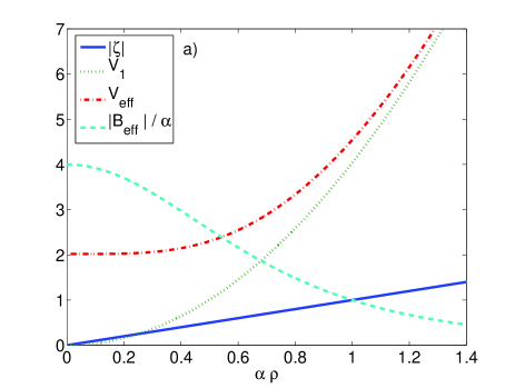
Figure 2: (Color online) Effective trapping potential $V_{\mathrm{eff}}$ and effective magnetic field $B_{\mathrm{eff}}$ for the case where $|\zeta|$ is linear in $\rho$ and the constants are $m=\hbar=1$, $\alpha=0.2$, $l=10$. The trapping potential $V_{1}$ is chosen to be given by Eq. (45), so that the quadratic term of the effective trapping potential vanishes. The trapping potential for the atoms in the second hyperfine ground state is chosen to be $V_{2}(\mathbf{r})=\kappa V_{1}(\mathbf{r})$ with (a) $\kappa=1$ and (b) $\kappa=7/3$.

Figure 2 shows the effective magnetic field and the trapping potential for the whole range of distances $\rho$ in the case where $V_{2}(\mathbf{r})=\kappa V_{1}(\mathbf{r})$, with $\kappa=1$ (Fig. 2a) and $\kappa=7/3$ (Fig. 2b). The external trapping potential is defined here by Eqs. (31) and (45). The overall trapping potential is seen to be flat for small distances ($\alpha\rho\ll 1$). In this area the magnetic field is close to its maximum value. For larger distances an effective trapping barrier is formed preventing the atoms to escape the area where the magnetic field is contained, as seen in Fig. 2. In other words, the atoms can be trapped in the area where the magnetic field is concentrated. For $\kappa=7/3$ the effective trapping potential confines the atoms tighter compared to the case where $\kappa=1$, as one can see comparing Figs. 2a and 2b.

Since the effective magnetic field is nearly constant only in a region where $|\zeta|=\alpha\rho\ll 1$, the effective magnetic flux over this region is much smaller than its maximum of $2\pi\hbar l$, as one can see from Eq. (39). In the next subsection we shall show how to produce a strictly constant magnetic field in the case where $|\zeta|$ is not necessarily small.

V.3 Constant effective magnetic field

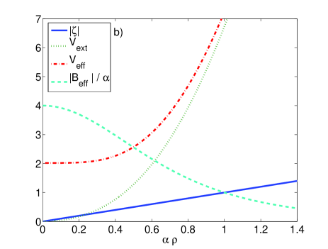
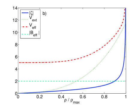
Figure 3: (Color online) The effective trapping potential $V_{\mathrm{eff}}$ and the ratio $|\zeta|=\left|\Omega_{p}/\Omega_{c}\right|$ corresponding to the case where the effective magnetic field $B_{\mathrm{eff}}$ is constant. The external trapping potential $V_{1}(\mathbf{r})$ is given by Eq. (50) to compensate the quadratic term in Eq. (49). The trapping potential for the atoms in the second hyperfine ground state is chosen to be $V_{2}(\mathbf{r})=\kappa V_{1}(\mathbf{r})$ with (a) $\kappa=1$ and (b) $\kappa=7/3$. The other constants are in both cases $m=\hbar=1$, $l=10$ and $\rho_{\mathrm{max}}^{2}=10$.

If we choose

$$|\zeta|^{2}=\frac{\left(\rho/\rho_{\mathrm{max}}\right)^{2}}{1-\left(\rho/\rho_{\mathrm{max}}\right)^{2}}\,,$$ (46)

the effective vector potential is

$$\mathbf{A}_{\mathrm{eff}}^{(D)}=-\hbar l\rho\rho_{\mathrm{max}}^{-2}\hat{\mathbf{e}}_{\phi}\,.$$ (47)

Consequently we arrive at a constant effective magnetic field

$$\mathbf{B}_{\mathrm{eff}}=-2\hbar l\rho_{\mathrm{max}}^{-2}\hat{\mathbf{e}}_{z}\,,$$ (48)

with the corresponding cyclotron frequency $\omega_{c}=\hbar 2l/m\rho_{\mathrm{max}}^{2}$, and the magnetic length $\ell_{B}=\sqrt{\hbar/m\omega_{c}}=\rho_{\mathrm{max}}/\sqrt{2l}$. The effective trapping potential is now given by

$$V_{\mathrm{eff}}^{(D)}(\mathbf{r})=V_{\mathrm{ext}}(\mathbf{r})+\frac{\hbar^{2}}{2m}\frac{1}{\rho_{\mathrm{max}}^{2}}\left(l^{2}d+1/d\right)\,,$$ (49)

where $d=1-\left(\rho/\rho_{\mathrm{max}}\right)^{2}$. For $\rho\rightarrow\rho_{\mathrm{max}}$, the intensity ratio $|\zeta|^{2}$ goes to infinity, so the equations (46)-(49) have a meaning only for distances smaller than $\rho_{\mathrm{max}}$. Therefore, Eq. (46) can model an actual intensity distribution of the control and probe beams only up to a certain radius $\rho_{0}$ which is smaller than $\rho_{\mathrm{max}}$. When the radius $\rho_{0}$ is close to $\rho_{\mathrm{max}}$, the effective magnetic flux approaches its maximum value of $2\pi\hbar l$.

If

$$V_{1}(\mathbf{r})=\frac{\hbar^{2}}{2m\rho_{\mathrm{max}}^{2}}\left(l^{2}-1\right)\left(\rho/\rho_{\mathrm{max}}\right)^{2}\,,$$ (50)

and $V_{2}(\mathbf{r})=\kappa V_{1}(\mathbf{r})$, the external potential $V_{\mathrm{ext}}(\mathbf{r})$ given by Eq. (31) compensates the quadratic term in Eq. (49). Assuming $\kappa=1$, the overall effective trapping potential $V_{\mathrm{eff}}^{(D)}(\mathbf{r})$ is flat almost up to the large limiting radius $\rho=\rho_{\mathrm{max}}$, as one can see from Fig. 3a. Figure 3b shows the situation where $\kappa=7/3$, so that the atoms in hyperfine state $2$ are trapped stronger. In this case, the effective trapping potential becomes tighter. Consequently, the difference in trapping potentials for different hyperfine states can provide a natural container confining the trapped atoms within an area of a constant effective magnetic field.

If the winding number of the probe beam $l_{p}=l$ is of the order of a hundred, the magnetic length $\ell_{B}=\rho_{\mathrm{max}}/\sqrt{l}$ can be considerably smaller than the width of an atomic cloud. On the other hand, the diameter of a pancake shaped cloud is normaly in the range of several tens of micrometers, and the ratio $\hbar/m$ is of the order of $1\mu\mathrm{m}^{2}/\mathrm{ms}$ for alkali atoms. Therefore, the cyclotron frequency $\omega_{c}=\hbar l/m\rho_{\mathrm{max}}^{2}$ can be up to several hundreds of Hz which is comparable to typical trapping frequencies.

VI Conclusions

We have considered the influence of two beams of light with orbital angular momenta on a degenerate gas of electrically neutral atoms (fermions or bosons). The theory is based on the EIT. We have derived an equation of motion for atoms driven to a dark state. The equation contains a vector potential type interaction as well as an effective trapping potential. We have analyzed the effective vector and trapping potentials in the case where at least one of the light beams contains an orbital angular momentum. We have shown how to generate a constant effective magnetic field, as well as a field exhibiting a radial distance dependence. We have demonstrated that the effective magnetic field can be concentrated in the area where the effective trapping potential holds the atoms. In the case of a homogeneous effective magnetic field it is important to realize that the corresponding cyclotron frequencies and magnetic lengths can be similar to typical trap frequencies and oscillator lengths used when trapping cold atoms in BEC and degenerate fermion gases. This will require a high OAM for the light which is also readily available with present technology.

The theory is based on the adiabatic approximation according to which the atoms should remain in the dark state. We have estimated that the adiabatic approximation should hold for atomic velocities up to tens of meters per second, i.e., up to extremely large velocities in the context of ultra-cold atomic gases. Such an estimate is lowered if the spontaneous decay of the excited atoms is taken into account. The atomic dark state accquires then a velocity-dependent lifetime. For instance, if the atomic velocities are of the order of a centimeter per second, the atoms should survive in their dark states up to a few seconds, which is comparable to a typical lifetime of an atomic BEC.

Our proposed method of creating the effective magnetic field has several advantages compared to a rotating system where only a constant magnetic field is created Bretin et al. (2004); Schweikhard et al. (2004); Baranov et al. (2005). In our method the magnetic field is shaped and controlled by choosing the proper control and probe beams. Furthermore stirring an ultra-cold cloud of atoms in a controlled manner is a rather demanding task, whereas an optically induced vector potential is expected to be highly controllable.

The theory has already been applied analyzing the de Haas-van Alphen effect in a gas of electrically neutral atoms Juzeliūnas and Öhberg (2004). It can also be applied to other intriguing phenomena which intrinsically depend on the magnetic field. For instance, the quantum Hall effect can now be studied using a cold gas of electrically neutral atomic fermions. In addition, if the collisional interaction between the atoms is taken into account, we can study the magnetic properties of a superfluid atomic Fermi gas Regal et al. (2004). Recent advances in spatial light modulator technology enables us to consider rather exotic light beams McGloin et al. (2003). This will allow us to study the effect of different forms of vector potentials in quantum gases. Finally the combined dynamical system of light and matter Öhberg (2002) could give an important insight into gauge theories in general.

Appendix A Equations of motion for $\Phi_{D}$ and $\Phi_{B}$

For derivation of the equations of motion for the dark and bright states $\Phi_{D}$ and $\Phi_{B}$ it is convenient to introduce the notation

$$\xi_{c}=\frac{1}{\sqrt{1+|\zeta|^{2}}}\,,\quad\xi_{p}=\frac{\zeta}{\sqrt{1+|\zeta|^{2}}}\,.$$ (51)

To obtain the equation for $\Phi_{D}$ and $\Phi_{B}$, let us take the time derivative of Eq. (8) and (9) and make use of the original equations of motion (3)-(5):

$$i\hbar\dot{\Phi}_{D} = -\frac{\hbar^{2}}{2m}\left(\xi_{c}^{*}\nabla^{2}\Phi_{1}-\xi_{p}^{*}\nabla^{2}\Phi_{2}\right)+\xi_{c}^{*}V_{1}(\mathbf{r})\Phi_{1}-\xi_{p}^{*}\left(\epsilon_{21}+V_{2}(\mathbf{r})\right)\Phi_{2}$$ (52)

$$+\dot{\xi}_{c}^{*}\Phi_{1}-\dot{\xi}_{p}^{*}\Phi_{2}\,,$$

$$i\hbar\dot{\Phi}_{B} = -\frac{\hbar^{2}}{2m}\left(\xi_{p}\nabla^{2}\Phi_{1}+\xi_{c}\nabla^{2}\Phi_{2}\right)+\xi_{p}V_{1}(\mathbf{r})\Phi_{1}+\xi_{c}\left(\epsilon_{21}+V_{2}(\mathbf{r})\right)\Phi_{2}$$ (53)

$$+\hbar\Omega\frac{\Omega_{c}^{*}}{|\Omega_{c}|}\Phi_{3}+\dot{\xi}_{p}\Phi_{1}+\dot{\xi}_{c}\Phi_{2}\,.$$

Using the inverse transformation

$$\Phi_{1}=\frac{1}{\sqrt{1+|\zeta|^{2}}}(\zeta^{*}\Phi_{B}+\Phi_{D})$$ (54)

and

$$\Phi_{2}=\frac{1}{\sqrt{1+|\zeta|^{2}}}(\Phi_{B}-\zeta\Phi_{D})\,,$$ (55)

the equations of motion can be represented as

$$i\hbar\dot{\Phi}_{D}=\frac{1}{2m}\left(-i\hbar\nabla-\mathbf{A}_{\mathrm{eff}}^{(D)}\right)^{2}\Phi_{D}+V_{\mathrm{eff}}^{(D)}(\mathbf{r})\Phi_{D}+F_{DB}(\mathbf{r})\Phi_{B}\,,$$ (56)

and

$$i\hbar\dot{\Phi}_{B}=\frac{1}{2m}\left(-i\hbar\nabla+\mathbf{A}_{\mathrm{eff}}^{(D)}\right)^{2}\Phi_{B}+V_{\mathrm{eff}}^{(B)}(\mathbf{r})\Phi_{B}+\hbar\Omega\frac{\Omega_{c}^{*}}{|\Omega_{c}|}\Phi_{3}+F_{BD}(\mathbf{r})\Phi_{D}\,,$$ (57)

where the effective vector and trapping potentials are explicitly defined by Eqs. (15)–(17) of the main text. The operators $F_{DB}(\mathbf{r})$ and $F_{BD}(\mathbf{r})$ describe the transitions between the dark and bright states:

$$F_{DB}(\mathbf{r})\Phi_{B} = \left[\left(V_{1}(\mathbf{r})-V_{2}(\mathbf{r})-\epsilon_{21}\right)\xi_{c}^{*}\xi_{p}^{*}+\frac{\hbar^{2}}{2m}\left(\xi_{p}^{*}\nabla^{2}\xi_{c}^{*}-\xi_{c}^{*}\nabla^{2}\xi_{p}^{*}\right)+i\hbar\left(\dot{\xi}_{c}^{*}\xi_{p}^{*}-\dot{\xi}_{p}^{*}\xi_{c}^{*}\right)\right]\Phi_{B}$$ (58)

$$+\frac{\hbar^{2}}{m}\left(\xi_{p}^{*}\nabla\xi_{c}^{*}-\xi_{c}^{*}\nabla\xi_{p}^{*}\right)\cdot\nabla\Phi_{B}\,,$$

$$F_{BD}(\mathbf{r})\Phi_{D} = \left[\left(V_{1}(\mathbf{r})-V_{2}(\mathbf{r})-\epsilon_{21}\right)\xi_{c}\xi_{p}+\frac{\hbar^{2}}{2m}\left(\xi_{c}\nabla^{2}\xi_{p}-\xi_{p}\nabla^{2}\xi_{c}\right)+i\hbar\left(\dot{\xi}_{p}\xi_{c}-\dot{\xi}_{c}\xi_{p}\right)\right]\Phi_{D}$$ (59)

$$+\frac{\hbar^{2}}{m}\left(\xi_{c}\nabla\xi_{p}-\xi_{p}\nabla\xi_{c}\right)\cdot\nabla\Phi_{D}\,.$$

Finally, substituting Eqs. (54) and (55) into Eq. (4), one arrives at Eq. (13) for $\Phi_{3}$.