Power laws, Pareto distributions and Zipf’s law

Abstract

When the probability of measuring a particular value of some quantity varies inversely as a power of that value, the quantity is said to follow a power law, also known variously as Zipf’s law or the Pareto distribution. Power laws appear widely in physics, biology, earth and planetary sciences, economics and finance, computer science, demography and the social sciences. For instance, the distributions of the sizes of cities, earthquakes, solar flares, moon craters, wars and people’s personal fortunes all appear to follow power laws. The origin of power-law behaviour has been a topic of debate in the scientific community for more than a century. Here we review some of the empirical evidence for the existence of power-law forms and the theories proposed to explain them.

I Introduction

Many of the things that scientists measure have a typical size or “scale”—a typical value around which individual measurements are centred. A simple example would be the heights of human beings. Most adult human beings are about 180cm tall. There is some variation around this figure, notably depending on sex, but we never see people who are 10cm tall, or 500cm. To make this observation more quantitative, one can plot a histogram of people’s heights, as I have done in Fig. 1a. The figure shows the heights in centimetres of adult men in the United States measured between 1959 and 1962, and indeed the distribution is relatively narrow and peaked around 180cm. Another telling observation is the ratio of the heights of the tallest and shortest people. The Guinness Book of Records claims the world’s tallest and shortest adult men (both now dead) as having had heights 272cm and 57cm respectively, making the ratio 4.8. This is a relatively low value; as we will see in a moment, some other quantities have much higher ratios of largest to smallest.

Figure 1b shows another example of a quantity with a typical scale: the speeds in miles per hour of cars on the motorway. Again the histogram of speeds is strongly peaked, in this case around 75mph.

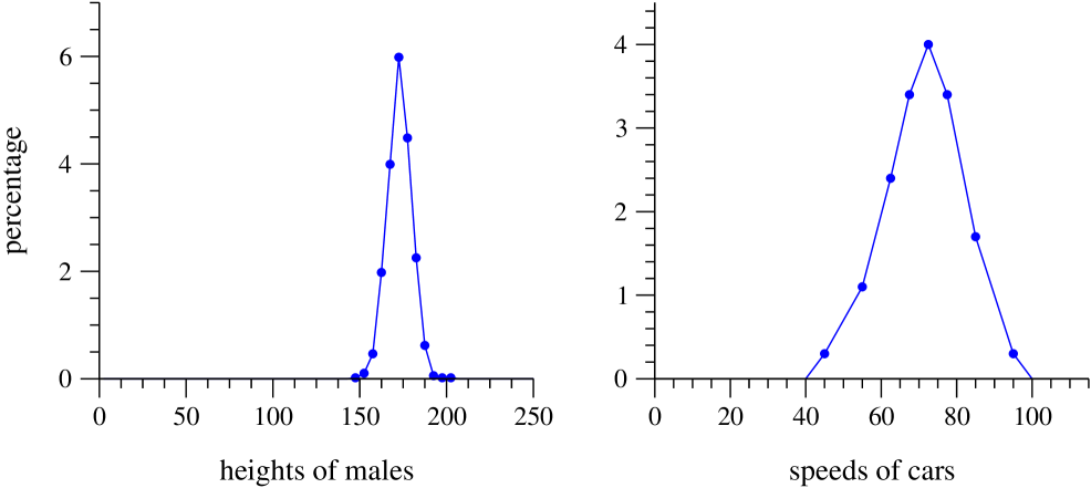
Figure 1: Left: histogram of heights in centimetres of American males. Data from the National Health Examination Survey, 1959–1962 (US Department of Health and Human Services). Right: histogram of speeds in miles per hour of cars on UK motorways. Data from Transport Statistics 2003 (UK Department for Transport).

But not all things we measure are peaked around a typical value. Some vary over an enormous dynamic range, sometimes many orders of magnitude. A classic example of this type of behaviour is the sizes of towns and cities. The largest population of any city in the US is 8.00 million for New York City, as of the most recent (2000) census. The town with the smallest population is harder to pin down, since it depends on what you call a town. The author recalls in 1993 passing through the town of Milliken, Oregon, population 4, which consisted of one large house occupied by the town’s entire human population, a wooden shack occupied by an extraordinary number of cats and a very impressive flea market. According to the Guinness Book, however, America’s smallest town is Duffield, Virginia, with a population of 52. Whichever way you look at it, the ratio of largest to smallest population is at least $150\,000$. Clearly this is quite different from what we saw for heights of people. And an even more startling pattern is revealed when we look at the histogram of the sizes of cities, which is shown in Fig. 2.

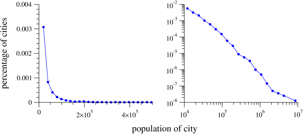
Figure 2: Left: histogram of the populations of all US cities with population of $10\,000$ or more. Right: another histogram of the same data, but plotted on logarithmic scales. The approximate straight-line form of the histogram in the right panel implies that the distribution follows a power law. Data from the 2000 US Census.

In the left panel of the figure, I show a simple histogram of the distribution of US city sizes. The histogram is highly right-skewed, meaning that while the bulk of the distribution occurs for fairly small sizes—most US cities have small populations—there is a small number of cities with population much higher than the typical value, producing the long tail to the right of the histogram. This right-skewed form is qualitatively quite different from the histograms of people’s heights, but is not itself very surprising. Given that we know there is a large dynamic range from the smallest to the largest city sizes, we can immediately deduce that there can only be a small number of very large cities. After all, in a country such as America with a total population of 300 million people, you could at most have about 40 cities the size of New York. And the 2700 cities in the histogram of Fig. 2 cannot have a mean population of more than $3\times 10^{8}/2700=110\,000$.

What is surprising on the other hand, is the right panel of Fig. 2, which shows the histogram of city sizes again, but this time replotted with logarithmic horizontal and vertical axes. Now a remarkable pattern emerges: the histogram, when plotted in this fashion, follows quite closely a straight line. This observation seems first to have been made by Auerbach [1], although it is often attributed to Zipf [2]. What does it mean? Let $p(x)\>{\rm d}x$ be the fraction of cities with population between $x$ and $x+{\rm d}x$. If the histogram is a straight line on log-log scales, then $\ln p(x)=-\alpha\ln x+c$, where $\alpha$ and $c$ are constants. (The minus sign is optional, but convenient since the slope of the line in Fig. 2 is clearly negative.) Taking the exponential of both sides, this is equivalent to:

$$p(x)=Cx^{-\alpha},$$ (1)

with $C={\rm e}^{c}$.

Distributions of the form (1) are said to follow a power law. The constant $\alpha$ is called the exponent of the power law. (The constant $C$ is mostly uninteresting; once $\alpha$ is fixed, it is determined by the requirement that the distribution $p(x)$ sum to 1; see Section III.1.)

Power-law distributions occur in an extraordinarily diverse range of phenomena. In addition to city populations, the sizes of earthquakes [3], moon craters [4], solar flares [5], computer files [6] and wars [7], the frequency of use of words in any human language [8, 2], the frequency of occurrence of personal names in most cultures [9], the numbers of papers scientists write [10], the number of citations received by papers [11], the number of hits on web pages [12], the sales of books, music recordings and almost every other branded commodity [13, 14], the numbers of species in biological taxa [15], people’s annual incomes [16] and a host of other variables all follow power-law distributions.

Power-law distributions are the subject of this article. In the following sections, I discuss ways of detecting power-law behaviour, give empirical evidence for power laws in a variety of systems and describe some of the mechanisms by which power-law behaviour can arise.

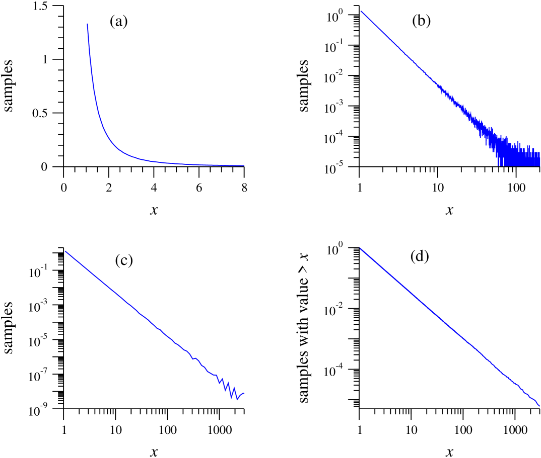
Figure 3: (a) Histogram of the set of 1 million random numbers described in the text, which have a power-law distribution with exponent $\alpha=2.5$. (b) The same histogram on logarithmic scales. Notice how noisy the results get in the tail towards the right-hand side of the panel. This happens because the number of samples in the bins becomes small and statistical fluctuations are therefore large as a fraction of sample number. (c) A histogram constructed using “logarithmic binning”. (d) A cumulative histogram or rank/frequency plot of the same data. The cumulative distribution also follows a power law, but with an exponent of $\alpha-1=1.5$.

Readers interested in pursuing the subject further may also wish to consult the reviews by Sornette [18] and Mitzenmacher [19], as well as the bibliography by Li.

II Measuring power laws

Identifying power-law behaviour in either natural or man-made systems can be tricky. The standard strategy makes use of a result we have already seen: a histogram of a quantity with a power-law distribution appears as a straight line when plotted on logarithmic scales. Just making a simple histogram, however, and plotting it on log scales to see if it looks straight is, in most cases, a poor way proceed.

Consider Fig. 3. This example shows a fake data set: I have generated a million random real numbers drawn from a power-law probability distribution $p(x)=Cx^{-\alpha}$ with exponent $\alpha=2.5$, just for illustrative purposes. Panel (a) of the figure shows a normal histogram of the numbers, produced by binning them into bins of equal size $0.1$. That is, the first bin goes from $1$ to $1.1$, the second from $1.1$ to $1.2$, and so forth. On the linear scales used this produces a nice smooth curve.

To reveal the power-law form of the distribution it is better, as we have seen, to plot the histogram on logarithmic scales, and when we do this for the current data we see the characteristic straight-line form of the power-law distribution, Fig. 3b. However, the plot is in some respects not a very good one. In particular the right-hand end of the distribution is noisy because of sampling errors. The power-law distribution dwindles in this region, meaning that each bin only has a few samples in it, if any. So the fractional fluctuations in the bin counts are large and this appears as a noisy curve on the plot. One way to deal with this would be simply to throw out the data in the tail of the curve. But there is often useful information in those data and furthermore, as we will see in Section II.1, many distributions follow a power law only in the tail, so we are in danger of throwing out the baby with the bathwater.

An alternative solution is to vary the width of the bins in the histogram. If we are going to do this, we must also normalize the sample counts by the width of the bins they fall in. That is, the number of samples in a bin of width $\Delta x$ should be divided by $\Delta x$ to get a count per unit interval of $x$. Then the normalized sample count becomes independent of bin width on average and we are free to vary the bin widths as we like. The most common choice is to create bins such that each is a fixed multiple wider than the one before it. This is known as logarithmic binning. For the present example, for instance, we might choose a multiplier of 2 and create bins that span the intervals 1 to $1.1$, $1.1$ to $1.3$, $1.3$ to $1.7$ and so forth (i.e., the sizes of the bins are $0.1$, $0.2$, $0.4$ and so forth). This means the bins in the tail of the distribution get more samples than they would if bin sizes were fixed, and this reduces the statistical errors in the tail. It also has the nice side-effect that the bins appear to be of constant width when we plot the histogram on log scales.

I used logarithmic binning in the construction of Fig. 2b, which is why the points representing the individual bins appear equally spaced. In Fig. 3c I have done the same for our computer-generated power-law data. As we can see, the straight-line power-law form of the histogram is now much clearer and can be seen to extend for at least a decade further than was apparent in Fig. 3b.

Even with logarithmic binning there is still some noise in the tail, although it is sharply decreased. Suppose the bottom of the lowest bin is at $x_{\mathrm{min}}$ and the ratio of the widths of successive bins is $a$. Then the $k$th bin extends from $x_{k-1}=x_{\mathrm{min}}a^{k-1}$ to $x_{k}=x_{\mathrm{min}}a^{k}$ and the expected number of samples falling in this interval is

$$\int_{x_{k-1}}^{x_{k}}\!p(x)\>{\rm d}x = C\int_{x_{k-1}}^{x_{k}}\!x^{-\alpha}\>{\rm d}x$$ (2)

$$= C\,{a^{\alpha-1}-1\over\alpha-1}(x_{\mathrm{min}}a^{k})^{-\alpha+1}.$$

Thus, so long as $\alpha>1$, the number of samples per bin goes down as $k$ increases and the bins in the tail will have more statistical noise than those that precede them. As we will see in the next section, most power-law distributions occurring in nature have $2\leq\alpha\leq 3$, so noisy tails are the norm.

Another, and in many ways a superior, method of plotting the data is to calculate a cumulative distribution function. Instead of plotting a simple histogram of the data, we make a plot of the probability $P(x)$ that $x$ has a value greater than or equal to $x$:

$$P(x)=\int_{x}^{\infty}p(x^{\prime})\>{\rm d}x^{\prime}.$$ (3)

The plot we get is no longer a simple representation of the distribution of the data, but it is useful nonetheless. If the distribution follows a power law $p(x)=Cx^{-\alpha}$, then

$$P(x)=C\int_{x}^{\infty}{x^{\prime}}^{-\alpha}\>{\rm d}x^{\prime}={C\over\alpha-1}x^{-(\alpha-1)}.$$ (4)

Thus the cumulative distribution function $P(x)$ also follows a power law, but with a different exponent $\alpha-1$, which is 1 less than the original exponent. Thus, if we plot $P(x)$ on logarithmic scales we should again get a straight line, but with a shallower slope.

But notice that there is no need to bin the data at all to calculate $P(x)$. By its definition, $P(x)$ is well-defined for every value of $x$ and so can be plotted as a perfectly normal function without binning. This avoids all questions about what sizes the bins should be. It also makes much better use of the data: binning of data lumps all samples within a given range together into the same bin and so throws out any information that was contained in the individual values of the samples within that range. Cumulative distributions don’t throw away any information; it’s all there in the plot.

Figure 3d shows our computer-generated power-law data as a cumulative distribution, and indeed we again see the tell-tale straight-line form of the power law, but with a shallower slope than before. Cumulative distributions like this are sometimes also called rank/frequency plots for reasons explained in Appendix A. Cumulative distributions with a power-law form are sometimes said to follow Zipf’s law or a Pareto distribution, after two early researchers who championed their study. Since power-law cumulative distributions imply a power-law form for $p(x)$, “Zipf’s law” and “Pareto distribution” are effectively synonymous with “power-law distribution”. (Zipf’s law and the Pareto distribution differ from one another in the way the cumulative distribution is plotted—Zipf made his plots with $x$ on the horizontal axis and $P(x)$ on the vertical one; Pareto did it the other way around. This causes much confusion in the literature, but the data depicted in the plots are of course identical.)

We know the value of the exponent $\alpha$ for our artificial data set since it was generated deliberately to have a particular value, but in practical situations we would often like to estimate $\alpha$ from observed data. One way to do this would be to fit the slope of the line in plots like Figs. 3b, c or d, and this is the most commonly used method. Unfortunately, it is known to introduce systematic biases into the value of the exponent [20], so it should not be relied upon. For example, a least-squares fit of a straight line to Fig. 3b gives $\alpha=2.26\pm 0.02$, which is clearly incompatible with the known value of $\alpha=2.5$ from which the data were generated.

An alternative, simple and reliable method for extracting the exponent is to employ the formula

$$\alpha=1+n\Biggl{[}\sum_{i=1}^{n}\ln{x_{i}\over x_{\mathrm{min}}}\Biggr{]}^{-1}.$$ (5)

Here the quantities $x_{i}$, $i=1\ldots n$ are the measured values of $x$ and $x_{\mathrm{min}}$ is again the minimum value of $x$. (As discussed in the following section, in practical situations $x_{\mathrm{min}}$ usually corresponds not to the smallest value of $x$ measured but to the smallest for which the power-law behaviour holds.) An estimate of the expected statistical error $\sigma$ on (5) is given by

$$\sigma=\sqrt{n}\Biggl{[}\sum_{i=1}^{n}\ln{x_{i}\over x_{\mathrm{min}}}\Biggr{]}^{-1}={\alpha-1\over\sqrt{n}}.$$ (6)

The derivation of both these formulas is given in Appendix B.

Applying Eqs. (5) and (6) to our present data gives an estimate of $\alpha=2.500\pm 0.002$ for the exponent, which agrees well with the known value of $2.5$.

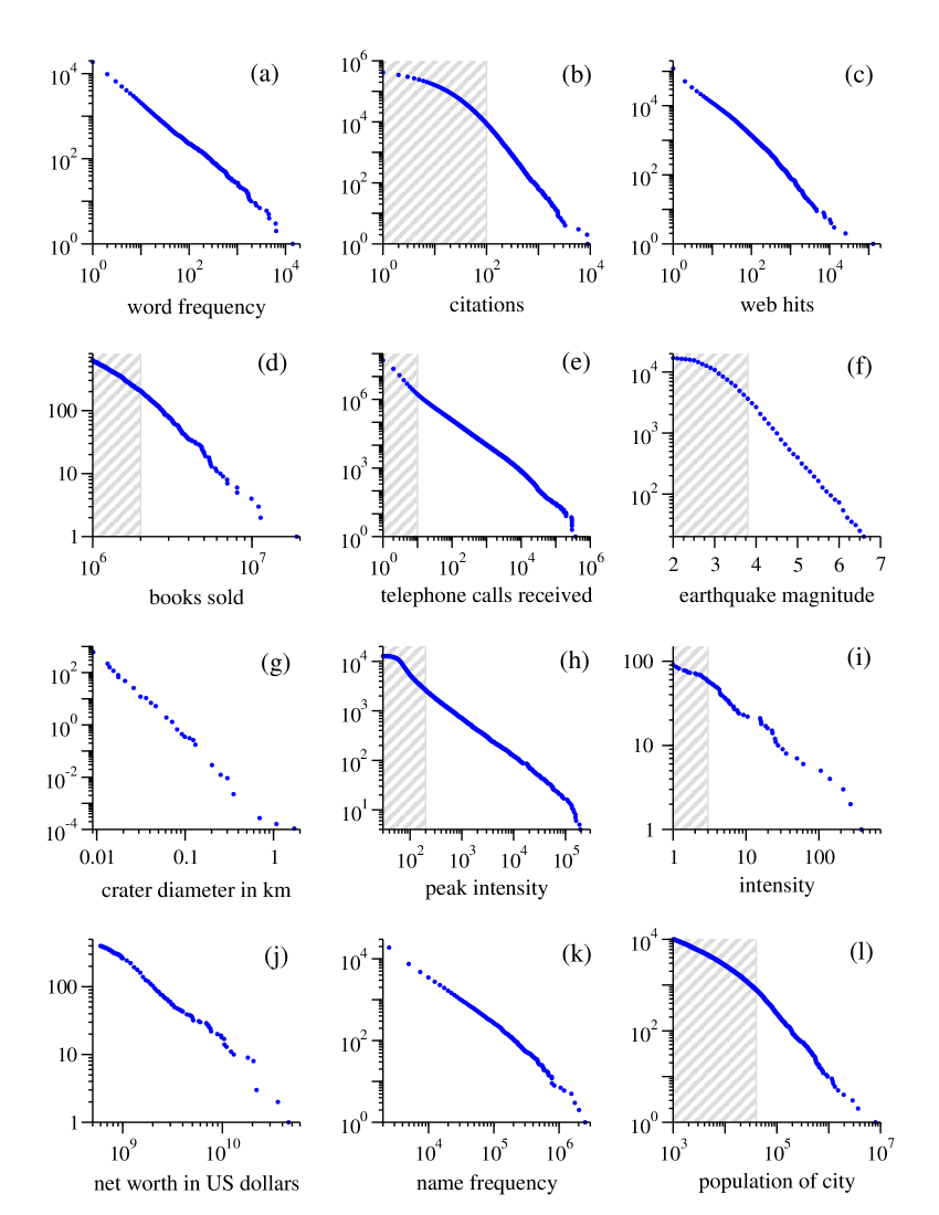
Figure 4: Cumulative distributions or “rank/frequency plots” of twelve quantities reputed to follow power laws. The distributions were computed as described in Appendix A. Data in the shaded regions were excluded from the calculations of the exponents in Table 1. Source references for the data are given in the text. (a) Numbers of occurrences of words in the novel Moby Dick by Hermann Melville. (b) Numbers of citations to scientific papers published in 1981, from time of publication until June 1997. (c) Numbers of hits on web sites by $60\,000$ users of the America Online Internet service for the day of 1 December 1997. (d) Numbers of copies of bestselling books sold in the US between 1895 and 1965. (e) Number of calls received by AT&T telephone customers in the US for a single day. (f) Magnitude of earthquakes in California between January 1910 and May 1992. Magnitude is proportional to the logarithm of the maximum amplitude of the earthquake, and hence the distribution obeys a power law even though the horizontal axis is linear. (g) Diameter of craters on the moon. Vertical axis is measured per square kilometre. (h) Peak gamma-ray intensity of solar flares in counts per second, measured from Earth orbit between February 1980 and November 1989. (i) Intensity of wars from 1816 to 1980, measured as battle deaths per $10\,000$ of the population of the participating countries. (j) Aggregate net worth in dollars of the richest individuals in the US in October 2003. (k) Frequency of occurrence of family names in the US in the year 1990. (l) Populations of US cities in the year 2000.

II.1 Examples of power laws

In Fig. 4 we show cumulative distributions of twelve different quantities measured in physical, biological, technological and social systems of various kinds. All have been proposed to follow power laws over some part of their range. The ubiquity of power-law behaviour in the natural world has led many scientists to wonder whether there is a single, simple, underlying mechanism linking all these different systems together. Several candidates for such mechanisms have been proposed, going by names like “self-organized criticality” and “highly optimized tolerance”. However, the conventional wisdom is that there are actually many different mechanisms for producing power laws and that different ones are applicable to different cases. We discuss these points further in Section IV.

The distributions shown in Fig. 4 are as follows.

1. Word frequency: Estoup [8] observed that the frequency with which words are used appears to follow a power law, and this observation was famously examined in depth and confirmed by Zipf [2]. Panel (a) of Fig. 4 shows the cumulative distribution of the number of times that words occur in a typical piece of English text, in this case the text of the novel Moby Dick by Herman Melville. Similar distributions are seen for words in other languages.

2. Citations of scientific papers: As first observed by Price [11], the numbers of citations received by scientific papers appear to have a power-law distribution. The data in panel (b) are taken from the Science Citation Index, as collated by Redner [22], and are for papers published in 1981. The plot shows the cumulative distribution of the number of citations received by a paper between publication and June 1997.

3. Web hits: The cumulative distribution of the number of “hits” received by web sites (i.e., servers, not pages) during a single day from a subset of the users of the AOL Internet service. The site with the most hits, by a long way, was yahoo.com. After Adamic and Huberman [12].

4. Copies of books sold: The cumulative distribution of the total number of copies sold in America of the 633 bestselling books that sold 2 million or more copies between 1895 and 1965. The data were compiled painstakingly over a period of several decades by Alice Hackett, an editor at Publisher’s Weekly [23]. The best selling book during the period covered was Benjamin Spock’s The Common Sense Book of Baby and Child Care. (The Bible, which certainly sold more copies, is not really a single book, but exists in many different translations, versions and publications, and was excluded by Hackett from her statistics.) Substantially better data on book sales than Hackett’s are now available from operations such as Nielsen BookScan, but unfortunately at a price this author cannot afford. I should be very interested to see a plot of sales figures from such a modern source.

5. Telephone calls: The cumulative distribution of the number of calls received on a single day by 51 million users of AT&T long distance telephone service in the United States. After Aiello et al. [24]. The largest number of calls received by a customer in that day was $375\,746$, or about 260 calls a minute (obviously to a telephone number that has many people manning the phones). Similar distributions are seen for the number of calls placed by users and also for the numbers of email messages that people send and receive [25, 26].

6. Magnitude of earthquakes: The cumulative distribution of the Richter (local) magnitude of earthquakes occurring in California between January 1910 and May 1992, as recorded in the Berkeley Earthquake Catalog. The Richter magnitude is defined as the logarithm, base 10, of the maximum amplitude of motion detected in the earthquake, and hence the horizontal scale in the plot, which is drawn as linear, is in effect a logarithmic scale of amplitude. The power law relationship in the earthquake distribution is thus a relationship between amplitude and frequency of occurrence. The data are from the National Geophysical Data Center, www.ngdc.noaa.gov.

7. Diameter of moon craters: The cumulative distribution of the diameter of moon craters. Rather than measuring the (integer) number of craters of a given size on the whole surface of the moon, the vertical axis is normalized to measure number of craters per square kilometre, which is why the axis goes below 1, unlike the rest of the plots, since it is entirely possible for there to be less than one crater of a given size per square kilometre. After Neukum and Ivanov [4].

8. Intensity of solar flares: The cumulative distribution of the peak gamma-ray intensity of solar flares. The observations were made between 1980 and 1989 by the instrument known as the Hard X-Ray Burst Spectrometer aboard the Solar Maximum Mission satellite launched in 1980. The spectrometer used a CsI scintillation detector to measure gamma-rays from solar flares and the horizontal axis in the figure is calibrated in terms of scintillation counts per second from this detector. The data are from the NASA Goddard Space Flight Center, umbra.nascom.nasa.gov/smm/hxrbs.html. See also Lu and Hamilton [5].

9. Intensity of wars: The cumulative distribution of the intensity of 119 wars from 1816 to 1980. Intensity is defined by taking the number of battle deaths among all participant countries in a war, dividing by the total combined populations of the countries and multiplying by $10\,000$. For instance, the intensities of the First and Second World Wars were $141.5$ and $106.3$ battle deaths per $10\,000$ respectively. The worst war of the period covered was the small but horrifically destructive Paraguay-Bolivia war of 1932–1935 with an intensity of $382.4$. The data are from Small and Singer [27]. See also Roberts and Turcotte [7].

10. Wealth of the richest people: The cumulative distribution of the total wealth of the richest people in the United States. Wealth is defined as aggregate net worth, i.e., total value in dollars at current market prices of all an individual’s holdings, minus their debts. For instance, when the data were compiled in 2003, America’s richest person, William H. Gates III, had an aggregate net worth of $46 billion, much of it in the form of stocks of the company he founded, Microsoft Corporation. Note that net worth doesn’t actually correspond to the amount of money individuals could spend if they wanted to: if Bill Gates were to sell all his Microsoft stock, for instance, or otherwise divest himself of any significant portion of it, it would certainly depress the stock price. The data are from Forbes magazine, 6 October 2003.

11. Frequencies of family names: Cumulative distribution of the frequency of occurrence in the US of the $89\,000$ most common family names, as recorded by the US Census Bureau in 1990. Similar distributions are observed for names in some other cultures as well (for example in Japan [28]) but not in all cases. Korean family names for instance appear to have an exponential distribution [29].

12. Populations of cities: Cumulative distribution of the size of the human populations of US cities as recorded by the US Census Bureau in 2000.

Few real-world distributions follow a power law over their entire range, and in particular not for smaller values of the variable being measured. As pointed out in the previous section, for any positive value of the exponent $\alpha$ the function $p(x)=Cx^{-\alpha}$ diverges as $x\to 0$. In reality therefore, the distribution must deviate from the power-law form below some minimum value $x_{\mathrm{min}}$. In our computer-generated example of the last section we simply cut off the distribution altogether below $x_{\mathrm{min}}$ so that $p(x)=0$ in this region, but most real-world examples are not that abrupt. Figure 4 shows distributions with a variety of behaviours for small values of the variable measured; the straight-line power-law form asserts itself only for the higher values. Thus one often hears it said that the distribution of such-and-such a quantity “has a power-law tail”.

Extracting a value for the exponent $\alpha$ from distributions like these can be a little tricky, since it requires us to make a judgement, sometimes imprecise, about the value $x_{\mathrm{min}}$ above which the distribution follows the power law. Once this judgement is made, however, $\alpha$ can be calculated simply from Eq. (5). (Care must be taken to use the correct value of $n$ in the formula; $n$ is the number of samples that actually go into the calculation, excluding those with values below $x_{\mathrm{min}}$, not the overall total number of samples.)

Table 1 lists the estimated exponents for each of the distributions of Fig. 4, along with standard errors and also the values of $x_{\mathrm{min}}$ used in the calculations. Note that the quoted errors correspond only to the statistical sampling error in the estimation of $\alpha$; they include no estimate of any errors introduced by the fact that a single power-law function may not be a good model for the data in some cases or for variation of the estimates with the value chosen for $x_{\mathrm{min}}$.

		minimum	exponent
	quantity	$x_{\mathrm{min}}$	$\alpha$
(a)	frequency of use of words	1	$2.20(1)$
(b)	number of citations to papers	100	$3.04(2)$
(c)	number of hits on web sites	1	$2.40(1)$
(d)	copies of books sold in the US	$2\,000\,000$	$3.51(16)$
(e)	telephone calls received	10	$2.22(1)$
(f)	magnitude of earthquakes	$3.8$	$3.04(4)$
(g)	diameter of moon craters	$0.01$	$3.14(5)$
(h)	intensity of solar flares	200	$1.83(2)$
(i)	intensity of wars	3	$1.80(9)$
(j)	net worth of Americans	$600m	$2.09(4)$
(k)	frequency of family names	$10\,000$	$1.94(1)$
(l)	population of US cities	$40\,000$	$2.30(5)$

Table 1: Parameters for the distributions shown in Fig. 4. The labels on the left refer to the panels in the figure. Exponent values were calculated using the maximum likelihood method of Eq. (5) and Appendix B, except for the moon craters (g), for which only cumulative data were available. For this case the exponent quoted is from a simple least-squares fit and should be treated with caution. Numbers in parentheses give the standard error on the trailing figures.

In the author’s opinion, the identification of some of the distributions in Fig. 4 as following power laws should be considered unconfirmed. While the power law seems to be an excellent model for most of the data sets depicted, a tenable case could be made that the distributions of web hits and family names might have two different power-law regimes with slightly different exponents. And the data for the numbers of copies of books sold cover rather a small range—little more than one decade horizontally. Nonetheless, one can, without stretching the interpretation of the data unreasonably, claim that power-law distributions have been observed in language, demography, commerce, information and computer sciences, geology, physics and astronomy, and this on its own is an extraordinary statement.

II.2 Distributions that do not follow a power law

Power-law distributions are, as we have seen, impressively ubiquitous, but they are not the only form of broad distribution. Lest I give the impression that everything interesting follows a power law, let me emphasize that there are quite a number of quantities with highly right-skewed distributions that nonetheless do not obey power laws. A few of them, shown in Fig. 5, are the following:

1. The abundance of North American bird species, which spans over five orders of magnitude but is probably distributed according to a log-normal. A log-normally distributed quantity is one whose logarithm is normally distributed; see Section IV.7 and Ref. [32] for further discussions.

2. The number of entries in people’s email address books, which spans about three orders of magnitude but seems to follow a stretched exponential. A stretched exponential is curve of the form ${\rm e}^{-ax^{b}}$ for some constants $a,b$.

3. The distribution of the sizes of forest fires, which spans six orders of magnitude and could follow a power law but with an exponential cutoff.

This being an article about power laws, I will not discuss further the possible explanations for these distributions, but the scientist confronted with a new set of data having a broad dynamic range and a highly skewed distribution should certainly bear in mind that a power-law model is only one of several possibilities for fitting it.

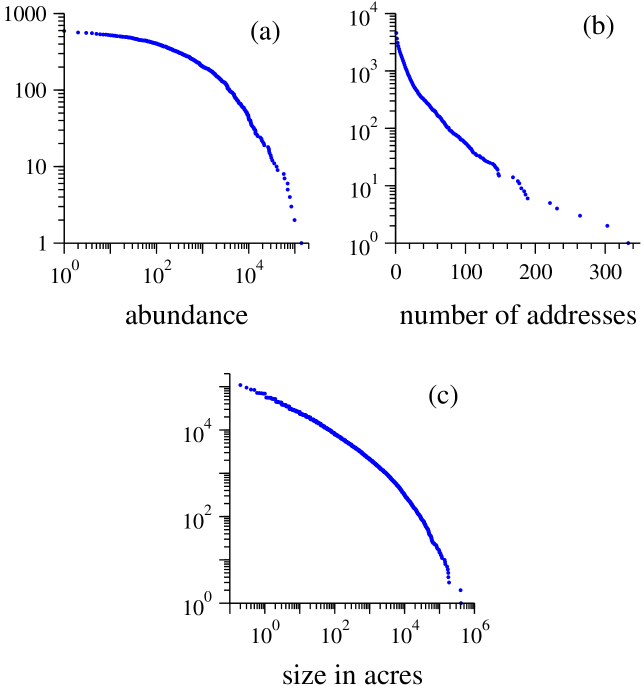
Figure 5: Cumulative distributions of some quantities whose distributions span several orders of magnitude but that nonetheless do not follow power laws. (a) The number of sightings of 591 species of birds in the North American Breeding Bird Survey 2003. (b) The number of addresses in the email address books of $16\,881$ users of a large university computer system [33]. (c) The size in acres of all wildfires occurring on US federal land between 1986 and 1996 (National Fire Occurrence Database, USDA Forest Service and Department of the Interior). Note that the horizontal axis is logarithmic in frames (a) and (c) but linear in frame (b).

III The mathematics of power laws

A continuous real variable with a power-law distribution has a probability $p(x)\>{\rm d}x$ of taking a value in the interval from $x$ to $x+{\rm d}x$, where

$$p(x)=Cx^{-\alpha},$$ (7)

with $\alpha>0$. As we saw in Section II.1, there must be some lowest value $x_{\mathrm{min}}$ at which the power law is obeyed, and we consider only the statistics of $x$ above this value.

III.1 Normalization

The constant $C$ in Eq. (7) is given by the normalization requirement that

$$1=\int_{x_{\mathrm{min}}}^{\infty}p(x)\>{\rm d}x=C\int_{x_{\mathrm{min}}}^{\infty}x^{-\alpha}\>{\rm d}x={C\over 1-\alpha}\Bigl{[}x^{-\alpha+1}\Bigr{]}_{x_{\mathrm{min}}}^{\infty}.$$ (8)

We see immediately that this only makes sense if $\alpha>1$, since otherwise the right-hand side of the equation would diverge: power laws with exponents less than unity cannot be normalized and don’t normally occur in nature. If $\alpha>1$ then Eq. (8) gives

$$C=(\alpha-1)x_{\mathrm{min}}^{\alpha-1},$$ (9)

and the correct normalized expression for the power law itself is

$$p(x)={\alpha-1\over x_{\mathrm{min}}}\,\biggl{(}{x\over x_{\mathrm{min}}}\biggr{)}^{-\alpha}.$$ (10)

Some distributions follow a power law for part of their range but are cut off at high values of $x$. That is, above some value they deviate from the power law and fall off quickly towards zero. If this happens, then the distribution may be normalizable no matter what the value of the exponent $\alpha$. Even so, exponents less than unity are rarely, if ever, seen.

III.2 Moments

The mean value of our power-law distributed quantity $x$ is given by

$$\left\langle x\right\rangle = \int_{x_{\mathrm{min}}}^{\infty}xp(x)\>{\rm d}x=C\int_{x_{\mathrm{min}}}^{\infty}x^{-\alpha+1}\>{\rm d}x$$ (11)

$$= {C\over 2-\alpha}\Bigl{[}x^{-\alpha+2}\Bigr{]}_{x_{\mathrm{min}}}^{\infty}.$$

Note that this expression becomes infinite if $\alpha\leq 2$. Power laws with such low values of $\alpha$ have no finite mean. The distributions of sizes of solar flares and wars in Table 1 are examples of such power laws.

What does it mean to say that a distribution has an infinite mean? Surely we can take the data for real solar flares and calculate their average? Indeed we can and necessarily we will always get a finite number from the calculation, since each individual measurement $x$ is itself a finite number and there are a finite number of them. Only if we had a truly infinite number of samples would we see the mean actually diverge.

However, if we were to repeat our finite experiment many times and calculate the mean for each repetition, then the mean of those many means is itself also formally divergent, since it is simply equal to the mean we would calculate if all the repetitions were combined into one large experiment. This implies that, while the mean may take a relatively small value on any particular repetition of the experiment, it must occasionally take a huge value, in order that the overall mean diverge as the number of repetitions does. Thus there must be very large fluctuations in the value of the mean, and this is what the divergence in Eq. (11) really implies. In effect, our calculations are telling us that the mean is not a well defined quantity, because it can vary enormously from one measurement to the next, and indeed can become arbitrarily large. The formal divergence of $\langle x\rangle$ is a signal that, while we can quote a figure for the average of the samples we measure, that figure is not a reliable guide to the typical size of the samples in another instance of the same experiment.

For $\alpha>2$ however, the mean is perfectly well defined, with a value given by Eq. (11) of

$$\left\langle x\right\rangle={\alpha-1\over\alpha-2}x_{\mathrm{min}}.$$ (12)

We can also calculate higher moments of the distribution $p(x)$. For instance, the second moment, the mean square, is given by

$$\left\langle x^{2}\right\rangle={C\over 3-\alpha}\Bigl{[}x^{-\alpha+3}\Bigr{]}_{x_{\mathrm{min}}}^{\infty}.$$ (13)

This diverges if $\alpha\leq 3$. Thus power-law distributions in this range, which includes almost all of those in Table 1, have no meaningful mean square, and thus also no meaningful variance or standard deviation. If $\alpha>3$, then the second moment is finite and well-defined, taking the value

$$\left\langle x^{2}\right\rangle={\alpha-1\over\alpha-3}x_{\mathrm{min}}^{2}.$$ (14)

These results can easily be extended to show that in general all moments $\left\langle x^{m}\right\rangle$ exist for $m<\alpha-1$ and all higher moments diverge. The ones that do exist are given by

$$\left\langle x^{m}\right\rangle={\alpha-1\over\alpha-1-m}x_{\mathrm{min}}^{m}.$$ (15)

III.3 Largest value

Suppose we draw $n$ measurements from a power-law distribution. What value is the largest of those measurements likely to take? Or, more precisely, what is the probability $\pi(x)\>{\rm d}x$ that the largest value falls in the interval between $x$ and $x+{\rm d}x$?

The definitive property of the largest value in a sample is that there are no others larger than it. The probability that a particular sample will be larger than $x$ is given by the quantity $P(x)$ defined in Eq. (3):

$$P(x)=\int_{x}^{\infty}p(x^{\prime})\>{\rm d}x^{\prime}={C\over\alpha-1}x^{-\alpha+1}=\biggl{(}{x\over x_{\mathrm{min}}}\biggr{)}^{-\alpha+1},$$ (16)

so long as $\alpha>1$. And the probability that a sample is not greater than $x$ is $1-P(x)$. Thus the probability that a particular sample we draw, sample $i$, will lie between $x$ and $x+{\rm d}x$ and that all the others will be no greater than it is $p(x)\>{\rm d}x\times[1-P(x)]^{n-1}$. Then there are $n$ ways to choose $i$, giving a total probability

$$\pi(x)=np(x)[1-P(x)]^{n-1}.$$ (17)

Now we can calculate the mean value $\left\langle x_{\mathrm{max}}\right\rangle$ of the largest sample thus:

$$\left\langle x_{\mathrm{max}}\right\rangle=\int_{x_{\mathrm{min}}}^{\infty}x\pi(x)\>{\rm d}x=n\int_{x_{\mathrm{min}}}^{\infty}xp(x)[1-P(x)]^{n-1}\>{\rm d}x.$$ (18)

Using Eqs. (10) and (16), this is

$$\left\langle x_{\mathrm{max}}\right\rangle = n(\alpha-1)\times$$ (19)

$$\hskip 3.99994pt\int_{x_{\mathrm{min}}}^{\infty}\biggl{(}{x\over x_{\mathrm{min}}}\biggr{)}^{-\alpha+1}\biggl{[}1-\biggl{(}{x\over x_{\mathrm{min}}}\biggr{)}^{-\alpha+1}\biggr{]}^{n-1}{\rm d}x$$

$$= nx_{\mathrm{min}}\int_{0}^{1}{y^{n-1}\over(1-y)^{1/(\alpha-1)}}\>{\rm d}y$$

$$= nx_{\mathrm{min}}\,\mathrm{B}\bigl{(}n,(\alpha-2)/(\alpha-1)\bigr{)},$$

where I have made the substitution $y=1-(x/x_{\mathrm{min}})^{-\alpha+1}$ and $\mathrm{B}(a,b)$ is Legendre’s beta-function, which is defined by

$$\mathrm{B}(a,b)={\Gamma(a)\Gamma(b)\over\Gamma(a+b)},$$ (20)

with $\Gamma(a)$ the standard $\Gamma$-function:

$$\Gamma(a)=\int_{0}^{\infty}t^{a-1}{\rm e}^{-t}\>{\rm d}t.$$ (21)

The beta-function has the interesting property that for large values of either of its arguments it itself follows a power law. For instance, for large $a$ and fixed $b$, $\mathrm{B}(a,b)\sim a^{-b}$. In most cases of interest, the number $n$ of samples from our power-law distribution will be large (meaning much greater than 1), so

$$\mathrm{B}\bigl{(}n,(\alpha-2)/(\alpha-1)\bigr{)}\sim n^{-(\alpha-2)/(\alpha-1)},$$ (22)

and

$$\left\langle x_{\mathrm{max}}\right\rangle\sim n^{1/(\alpha-1)}.$$ (23)

Thus, as long as $\alpha>1$, we find that $\left\langle x_{\mathrm{max}}\right\rangle$ always increases as $n$ becomes larger.

III.4 Top-heavy distributions and the 80/20 rule

Another interesting question is where the majority of the distribution of $x$ lies. For any power law with exponent $\alpha>1$, the median is well defined. That is, there is a point $x_{1/2}$ that divides the distribution in half so that half the measured values of $x$ lie above $x_{1/2}$ and half lie below. That point is given by

$$\int_{x_{1/2}}^{\infty}p(x)\>{\rm d}x=\mbox{$\frac{1}{2}$}\int_{x_{\mathrm{min}}}^{\infty}p(x)\>{\rm d}x,$$ (24)

or

$$x_{1/2}=2^{1/(\alpha-1)}x_{\mathrm{min}}.$$ (25)

So, for example, if we are considering the distribution of wealth, there will be some well-defined median wealth that divides the richer half of the population from the poorer. But we can also ask how much of the wealth itself lies in those two halves. Obviously more than half of the total amount of money belongs to the richer half of the population. The fraction of the money in the richer half is given by

$${\int_{x_{1/2}}^{\infty}xp(x)\>{\rm d}x\over\int_{x_{\mathrm{min}}}^{\infty}xp(x)\>{\rm d}x}=\biggl{(}{x_{1/2}\over x_{\mathrm{min}}}\biggr{)}^{-\alpha+2}=2^{-(\alpha-2)/(\alpha-1)},$$ (26)

provided $\alpha>2$ so that the integrals converge. Thus, for instance, if $\alpha=2.1$ for the wealth distribution, as indicated in Table 1, then a fraction $2^{-0.091}\simeq 94\%$ of the wealth is in the hands of the richer 50% of the population, making the distribution quite top-heavy.

More generally, the fraction of the population whose personal wealth exceeds $x$ is given by the quantity $P(x)$, Eq. (16), and the fraction of the total wealth in the hands of those people is

$$W(x)={\int_{x}^{\infty}x^{\prime}p(x^{\prime})\>{\rm d}x^{\prime}\over\int_{x_{\mathrm{min}}}^{\infty}x^{\prime}p(x^{\prime})\>{\rm d}x^{\prime}}=\biggl{(}{x\over x_{\mathrm{min}}}\biggr{)}^{-\alpha+2},$$ (27)

assuming again that $\alpha>2$. Eliminating $x/x_{\mathrm{min}}$ between (16) and (27), we find that the fraction $W$ of the wealth in the hands of the richest $P$ of the population is

$$W=P^{(\alpha-2)/(\alpha-1)},$$ (28)

of which Eq. (26) is a special case. This again has a power-law form, but with a positive exponent now. In Fig. 6 I show the form of the curve of $W$ against $P$ for various values of $\alpha$. For all values of $\alpha$ the curve is concave downwards, and for values only a little above 2 the curve has a very fast initial increase, meaning that a large fraction of the wealth is concentrated in the hands of a small fraction of the population. Curves of this kind are called Lorenz curves, after Max Lorenz, who first studied them around the turn of the twentieth century [34].

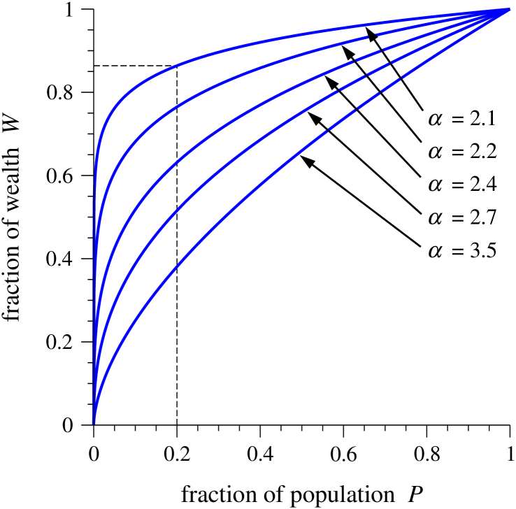
Figure 6: The fraction $W$ of the total wealth in a country held by the fraction $P$ of the richest people, if wealth is distributed following a power law with exponent $\alpha$. If $\alpha=2.1$, for instance, as it appears to in the United States (Table 1), then the richest 20% of the population hold about 86% of the wealth (dashed lines).

Using the exponents from Table 1, we can for example calculate that about 80% of the wealth should be in the hands of the richest 20% of the population (the so-called “80/20 rule”, which is borne out by more detailed observations of the wealth distribution), the top 20% of web sites get about two-thirds of all web hits, and the largest 10% of US cities house about 60% of the country’s total population.

If $\alpha\leq 2$ then the situation becomes even more extreme. In that case, the integrals in Eq. (27) diverge at their upper limits, meaning that in fact they depend on the value of the largest sample, as described in Section III.2. But for $\alpha>1$, Eq. (23) tells us that the expected value of $x_{\mathrm{max}}$ goes to $\infty$ as $n$ becomes large, and in that limit the fraction of money in the top half of the population, Eq. (26), tends to unity. In fact, the fraction of money in the top anything of the population, even the top 1%, tends to unity, as Eq. (27) shows. In other words, for distributions with $\alpha<2$, essentially all of the wealth (or other commodity) lies in the tail of the distribution. The distribution of family names in the US, which has an exponent $\alpha=1.9$, is an example of this type of behaviour. For the data of Fig. 4k, about 75% of the population have names in the top $15\,000$. Estimates of the total number of unique family names in the US put the figure at around 1.5 million. So in this case 75% of the population have names in the most common 1%—a very top-heavy distribution indeed. The line $\alpha=2$ thus separates the regime in which you will with some frequency meet people with uncommon names from the regime in which you will rarely meet such people.

III.5 Scale-free distributions

A power-law distribution is also sometimes called a scale-free distribution. Why? Because a power law is the only distribution that is the same whatever scale we look at it on. By this we mean the following.

Suppose we have some probability distribution $p(x)$ for a quantity $x$, and suppose we discover or somehow deduce that it satisfies the property that

$$p(bx)=g(b)p(x),$$ (29)

for any $b$. That is, if we increase the scale or units by which we measure $x$ by a factor of $b$, the shape of the distribution $p(x)$ is unchanged, except for an overall multiplicative constant. Thus for instance, we might find that computer files of size 2kB are $\frac{1}{4}$ as common as files of size 1kB. Switching to measuring size in megabytes we also find that files of size 2MB are $\frac{1}{4}$ as common as files of size 1MB. Thus the shape of the file-size distribution curve (at least for these particular values) does not depend on the scale on which we measure file size.

This scale-free property is certainly not true of most distributions. It is not true for instance of the exponential distribution. In fact, as we now show, it is only true of one type of distribution, the power law.

Starting from Eq. (29), let us first set $x=1$, giving $p(b)=g(b)p(1)$. Thus $g(b)=p(b)/p(1)$ and (29) can be written as

$$p(bx)={p(b)p(x)\over p(1)}.$$ (30)

Since this equation is supposed to be true for any $b$, we can differentiate both sides with respect to $b$ to get

$$xp^{\prime}(bx)={p^{\prime}(b)p(x)\over p(1)},$$ (31)

where $p^{\prime}$ indicates the derivative of $p$ with respect to its argument. Now we set $b=1$ and get

$$x{{\rm d}p\over{\rm d}x}={p^{\prime}(1)\over p(1)}p(x).$$ (32)

This is a simple first-order differential equation which has the solution

$$\ln p(x)={p(1)\over p^{\prime}(1)}\ln x+\mbox{constant}.$$ (33)

Setting $x=1$ we find that the constant is simply $\ln p(1)$, and then taking exponentials of both sides

$$p(x)=p(1)\,x^{-\alpha},$$ (34)

where $\alpha=-p(1)/p^{\prime}(1)$. Thus, as advertised, the power-law distribution is the only function satisfying the scale-free criterion (29).

This fact is more than just a curiosity. As we will see in Section IV.5, there are some systems that become scale-free for certain special values of their governing parameters. The point defined by such a special value is called a “continuous phase transition” and the argument given above implies that at such a point the observable quantities in the system should adopt a power-law distribution. This indeed is seen experimentally and the distributions so generated provided the original motivation for the study of power laws in physics (although most experimentally observed power laws are probably not the result of phase transitions—a variety of other mechanisms produce power-law behaviour as well, as we will shortly see).

III.6 Power laws for discrete variables

So far I have focused on power-law distributions for continuous real variables, but many of the quantities we deal with in practical situations are in fact discrete—usually integers. For instance, populations of cities, numbers of citations to papers or numbers of copies of books sold are all integer quantities. In most cases, the distinction is not very important. The power law is obeyed only in the tail of the distribution where the values measured are so large that, to all intents and purposes, they can be considered continuous. Technically however, power-law distributions should be defined slightly differently for integer quantities.

If $k$ is an integer variable, then one way to proceed is to declare that it follows a power law if the probability $p_{k}$ of measuring the value $k$ obeys

$$p_{k}=Ck^{-\alpha},$$ (35)

for some constant exponent $\alpha$. Clearly this distribution cannot hold all the way down to $k=0$, since it diverges there, but it could in theory hold down to $k=1$. If we discard any data for $k=0$, the constant $C$ would then be given by the normalization condition

$$1=\sum_{k=1}^{\infty}p_{k}=C\sum_{k=1}^{\infty}k^{-\alpha}=C\zeta(\alpha),$$ (36)

where $\zeta(\alpha)$ is the Riemann $\zeta$-function. Rearranging, we find that $C=1/\zeta(\alpha)$ and

$$p_{k}={k^{-\alpha}\over\zeta(\alpha)}.$$ (37)

If, as is usually the case, the power-law behaviour is seen only in the tail of the distribution, for values $k\geq k_{\mathrm{min}}$, then the equivalent expression is

$$p_{k}={k^{-\alpha}\over\zeta(\alpha,k_{\mathrm{min}})},$$ (38)

where $\zeta(\alpha,k_{\mathrm{min}})=\sum_{k=k_{\mathrm{min}}}^{\infty}k^{-\alpha}$ is the generalized or incomplete $\zeta$-function.

Most of the results of the previous sections can be generalized to the case of discrete variables, although the mathematics is usually harder and often involves special functions in place of the more tractable integrals of the continuous case.

It has occasionally been proposed that Eq. (35) is not the best generalization of the power law to the discrete case. An alternative and often more convenient form is

$$p_{k}=C\,{\Gamma(k)\Gamma(\alpha)\over\Gamma(k+\alpha)}=C\,\mathrm{B}(k,\alpha),$$ (39)

where $\mathrm{B}(a,b)$ is, as before, the Legendre beta-function, Eq. (20). As mentioned in Section III.3, the beta-function behaves as a power law $\mathrm{B}(k,\alpha)\sim k^{-\alpha}$ for large $k$ and so the distribution has the desired asymptotic form. Simon [35] proposed that Eq. (39) be called the Yule distribution, after Udny Yule who derived it as the limiting distribution in a certain stochastic process [36], and this name is often used today. Yule’s result is described in Section IV.4.

The Yule distribution is nice because sums involving it can frequently be performed in closed form, where sums involving Eq. (35) can only be written in terms of special functions. For instance, the normalizing constant $C$ for the Yule distribution is given by

$$1=C\sum_{k=1}^{\infty}\mathrm{B}(k,\alpha)={C\over\alpha-1},$$ (40)

and hence $C=\alpha-1$ and

$$p_{k}=(\alpha-1)\,\mathrm{B}(k,\alpha).$$ (41)

The first and second moments (i.e., the mean and mean square of the distribution) are

$$\left\langle k\right\rangle={\alpha-1\over\alpha-2},\qquad\left\langle k^{2}\right\rangle={(\alpha-1)^{2}\over(\alpha-2)(\alpha-3)},$$ (42)

and there are similarly simple expressions corresponding to many of our earlier results for the continuous case.

IV Mechanisms for generating power-law distributions

In this section we look at possible candidate mechanisms by which power-law distributions might arise in natural and man-made systems. Some of the possibilities that have been suggested are quite complex—notably the physics of critical phenomena and the tools of the renormalization group that are used to analyse it. But let us start with some simple algebraic methods of generating power-law functions and progress to the more involved mechanisms later.

IV.1 Combinations of exponentials

A much more common distribution than the power law is the exponential, which arises in many circumstances, such as survival times for decaying atomic nuclei or the Boltzmann distribution of energies in statistical mechanics. Suppose some quantity $y$ has an exponential distribution:

$$p(y)\sim{\rm e}^{ay}.$$ (43)

The constant $a$ might be either negative or positive. If it is positive then there must also be a cutoff on the distribution—a limit on the maximum value of $y$—so that the distribution is normalizable.

Now suppose that the real quantity we are interested in is not $y$ but some other quantity $x$, which is exponentially related to $y$ thus:

$$x\sim{\rm e}^{by},$$ (44)

with $b$ another constant, also either positive or negative. Then the probability distribution of $x$ is

$$p(x)=p(y){{\rm d}y\over{\rm d}x}\sim{{\rm e}^{ay}\over b{\rm e}^{by}}={x^{-1+a/b}\over b},$$ (45)

which is a power law with exponent $\alpha=1-a/b$.

A version of this mechanism was used by Miller [37] to explain the power-law distribution of the frequencies of words as follows (see also [38]). Suppose we type randomly on a typewriter, pressing the space bar with probability $q_{s}$ per stroke and each letter with equal probability $q_{l}$ per stroke. If there are $m$ letters in the alphabet then $q_{l}=(1-q_{s})/m$. (In this simplest version of the argument we also type no punctuation, digits or other non-letter symbols.) Then the frequency $x$ with which a particular word with $y$ letters (followed by a space) occurs is

$$x=\biggl{[}{1-q_{s}\over m}\biggr{]}^{y}q_{s}\sim{\rm e}^{by},$$ (46)

where $b=\ln(1-q_{s})-\ln m$. The number (or fraction) of distinct possible words with length between $y$ and $y+{\rm d}y$ goes up exponentially as $p(y)\sim m^{y}={\rm e}^{ay}$ with $a=\ln m$. Thus, following our argument above, the distribution of frequencies of words has the form $p(x)\sim x^{-\alpha}$ with

$$\alpha=1-{a\over b}={2\ln m-\ln(1-q_{s})\over\ln m-\ln(1-q_{s})}.$$ (47)

For the typical case where $m$ is reasonably large and $q_{s}$ quite small this gives $\alpha\simeq 2$ in approximate agreement with Table 1.

This is a reasonable theory as far as it goes, but real text is not made up of random letters. Most combinations of letters don’t occur in natural languages; most are not even pronounceable. We might imagine that some constant fraction of possible letter sequences of a given length would correspond to real words and the argument above would then work just fine when applied to that fraction, but upon reflection this suggestion is obviously bogus. It is clear for instance that very long words simply don’t exist in most languages, although there are exponentially many possible combinations of letters available to make them up. This observation is backed up by empirical data. In Fig. 7a we show a histogram of the lengths of words occurring in the text of Moby Dick, and one would need a particularly vivid imagination to convince oneself that this histogram follows anything like the exponential assumed by Miller’s argument. (In fact, the curve appears roughly to follow a log-normal [32].)

There may still be some merit in Miller’s argument however. The problem may be that we are measuring word “length” in the wrong units. Letters are not really the basic units of language. Some basic units are letters, but some are groups of letters. The letters “th” for example often occur together in English and make a single sound, so perhaps they should be considered to be a separate symbol in their own right and contribute only one unit to the word length?

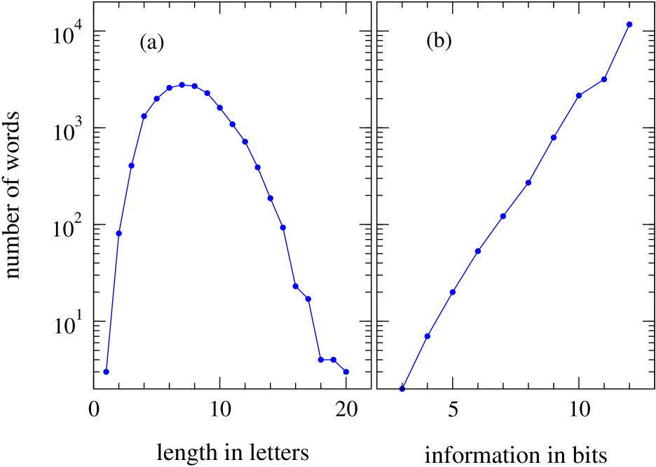
Figure 7: (a) Histogram of the lengths in letters of all distinct words in the text of the novel Moby Dick. (b) Histogram of the information content a la Shannon of words in Moby Dick. The former does not, by any stretch of the imagination, follow an exponential, but the latter could easily be said to do so. (Note that the vertical axes are logarithmic.)

Following this idea to its logical conclusion we can imagine replacing each fundamental unit of the language—whatever that is—by its own symbol and then measuring lengths in terms of numbers of symbols. The pursuit of ideas along these lines led Claude Shannon in the 1940s to develop the field of information theory, which gives a precise prescription for calculating the number of symbols necessary to transmit words or any other data [39, 40]. The units of information are bits and the true “length” of a word can be considered to be the number of bits of information it carries. Shannon showed that if we regard words as the basic divisions of a message, the information $y$ carried by any particular word is

$$y=-k\ln x,$$ (48)

where $x$ is the frequency of the word as before and $k$ is a constant. (The reader interested in finding out more about where this simple relation comes from is recommended to look at the excellent introduction to information theory by Cover and Thomas [41].)

But this has precisely the form that we want. Inverting it we have $x={\rm e}^{-y/k}$ and if the probability distribution of the “lengths” measured in terms of bits is also exponential as in Eq. (43) we will get our power-law distribution. Figure 7b shows the latter distribution, and indeed it follows a nice exponential—much better than Fig. 7a.

This is still not an entirely satisfactory explanation. Having made the shift from pure word length to information content, our simple count of the number of words of length $y$—that it goes exponentially as $m^{y}$—is no longer valid, and now we need some reason why there should be exponentially more distinct words in the language of high information content than of low. That this is the case is experimentally verified by Fig. 7b, but the reason must be considered still a matter of debate. Some possibilities are discussed by, for instance, Mandelbrot [42] and more recently by Mitzenmacher [19].

Another example of the “combination of exponentials” mechanism has been discussed by Reed and Hughes [43]. They consider a process in which a set of items, piles or groups each grows exponentially in time, having size $x\sim{\rm e}^{bt}$ with $b>0$. For instance, populations of organisms reproducing freely without resource constraints grow exponentially. Items also have some fixed probability of dying per unit time (populations might have a stochastically constant probability of extinction), so that the times $t$ at which they die are exponentially distributed $p(t)\sim{\rm e}^{at}$ with $a<0$.

These functions again follow the form of Eqs. (43) and (44) and result in a power-law distribution of the sizes $x$ of the items or groups at the time they die. Reed and Hughes suggest that variations on this argument may explain the sizes of biological taxa, incomes and cities, among other things.

IV.2 Inverses of quantities

Suppose some quantity $y$ has a distribution $p(y)$ that passes through zero, thus having both positive and negative values. And suppose further that the quantity we are really interested in is the reciprocal $x=1/y$, which will have distribution

$$p(x)=p(y){{\rm d}y\over{\rm d}x}=-{p(y)\over x^{2}}.$$ (49)

The large values of $x$, those in the tail of the distribution, correspond to the small values of $y$ close to zero and thus the large-$x$ tail is given by

$$p(x)\sim x^{-2},$$ (50)

where the constant of proportionality is $p(y=0)$.

More generally, any quantity $x=y^{-\gamma}$ for some $\gamma$ will have a power-law tail to its distribution $p(x)\sim x^{-\alpha}$, with $\alpha=1+1/\gamma$. It is not clear who the first author or authors were to describe this mechanism, but clear descriptions have been given recently by Bouchaud [44], Jan et al. [45] and Sornette [46].

One might argue that this mechanism merely generates a power law by assuming another one: the power-law relationship between $x$ and $y$ generates a power-law distribution for $x$. This is true, but the point is that the mechanism takes some physical power-law relationship between $x$ and $y$—not a stochastic probability distribution—and from that generates a power-law probability distribution. This is a non-trivial result.

One circumstance in which this mechanism arises is in measurements of the fractional change in a quantity. For instance, Jan et al. [45] consider one of the most famous systems in theoretical physics, the Ising model of a magnet. In its paramagnetic phase, the Ising model has a magnetization that fluctuates around zero. Suppose we measure the magnetization $m$ at uniform intervals and calculate the fractional change $\delta=(\Delta m)/m$ between each successive pair of measurements. The change $\Delta m$ is roughly normally distributed and has a typical size set by the width of that normal distribution. The $1/m$ on the other hand produces a power-law tail when small values of $m$ coincide with large values of $\Delta m$, so that the tail of the distribution of $\delta$ follows $p(\delta)\sim\delta^{-2}$ as above.

In Fig. 8 I show a cumulative histogram of measurements of $\delta$ for simulations of the Ising model on a square lattice, and the power-law distribution is clearly visible. Using Eq. (5), the value of the exponent is $\alpha=1.98\pm 0.04$, in good agreement with the expected value of 2.

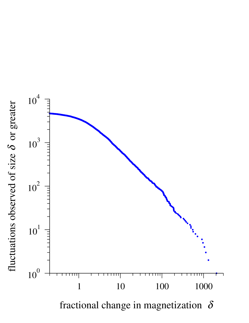
Figure 8: Cumulative histogram of the magnetization fluctuations of a $128\times 128$ nearest-neighbour Ising model on a square lattice. The model was simulated at a temperature of $2.5$ times the spin-spin coupling for $100\,000$ time steps using the cluster algorithm of Swendsen and Wang [47] and the magnetization per spin measured at intervals of ten steps. The fluctuations were calculated as the ratio $\delta_{i}=2(m_{i+1}-m_{i})/(m_{i+1}+m_{i})$.

IV.3 Random walks

Many properties of random walks are distributed according to power laws, and this could explain some power-law distributions observed in nature. In particular, a randomly fluctuating process that undergoes “gambler’s ruin”, i.e., that ends when it hits zero, has a power-law distribution of possible lifetimes.

Consider a random walk in one dimension, in which a walker takes a single step randomly one way or the other along a line in each unit of time. Suppose the walker starts at position 0 on the line and let us ask what the probability is that the walker returns to position 0 for the first time at time $t$ (i.e., after exactly $t$ steps). This is the so-called first return time of the walk and represents the lifetime of a gambler’s ruin process. A trick for answering this question is depicted in Fig. 9. We consider first the unconstrained problem in which the walk is allowed to return to zero as many times as it likes, before returning there again at time $t$. Let us denote the probability of this event as $u_{t}$. Let us also denote by $f_{t}$ the probability that the first return time is $t$. We note that both of these probabilities are non-zero only for even values of their arguments since there is no way to get back to zero in any odd number of steps.

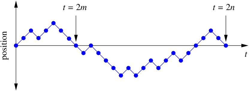
Figure 9: The position of a one-dimensional random walker (vertical axis) as a function of time (horizontal axis). The probability $u_{2n}$ that the walk returns to zero at time $t=2n$ is equal to the probability $f_{2m}$ that it returns to zero for the first time at some earlier time $t=2m$, multiplied by the probability $u_{2n-2m}$ that it returns again a time $2n-2m$ later, summed over all possible values of $m$. We can use this observation to write a consistency relation, Eq. (51), that can be solved for $f_{t}$, Eq. (59).

As Fig. 9 illustrates, the probability $u_{t}=u_{2n}$, with $n$ integer, can be written

$$u_{2n}=\biggl{\{}\begin{array}[]{ll}1&\qquad\mbox{if $n=0$,}\\ \sum_{m=1}^{n}f_{2m}u_{2n-2m}&\qquad\mbox{if $n\geq 1$,}\end{array}$$ (51)

where $m$ is also an integer and we define $f_{0}=0$ and $u_{0}=1$. This equation can conveniently be solved for $f_{2n}$ using a generating function approach. We define

$$U(z)=\sum_{n=0}^{\infty}u_{2n}z^{n},\quad F(z)=\sum_{n=1}^{\infty}f_{2n}z^{n}.$$ (52)

Then, multiplying Eq. (51) throughout by $z^{n}$ and summing, we find

$$U(z) = 1+\sum_{n=1}^{\infty}\sum_{m=1}^{n}f_{2m}u_{2n-2m}z^{n}$$ (53)

$$= 1+\sum_{m=1}^{\infty}f_{2m}z^{m}\sum_{n=m}^{\infty}u_{2n-2m}z^{n-m}$$

$$= 1+F(z)U(z).$$

So

$$F(z)=1-{1\over U(z)}.$$ (54)

The function $U(z)$ however is quite easy to calculate. The probability $u_{2n}$ that we are at position zero after $2n$ steps is

$$u_{2n}=2^{-2n}{2n\choose n},$$ (55)

so

$$U(z)=\sum_{n=0}^{\infty}{2n\choose n}{z^{n}\over 4^{n}}={1\over\sqrt{1-z}}.$$ (56)

And hence

$$F(z)={1-\sqrt{1-z}}.$$ (57)

Expanding this function using the binomial theorem thus:

$$F(z) = \mbox{$\frac{1}{2}$}z+{\mbox{$\frac{1}{2}$}\times\mbox{$\frac{1}{2}$}\over 2!}z^{2}+{\mbox{$\frac{1}{2}$}\times\mbox{$\frac{1}{2}$}\times\frac{3}{2}\over 3!}z^{3}+\ldots$$ (58)

$$= \sum_{n=1}^{\infty}{{2n\choose n}\over(2n-1)\,2^{2n}}z^{n}$$

and comparing this expression with Eq. (52), we immediately see that

$$f_{2n}={{2n\choose n}\over(2n-1)\,2^{2n}},$$ (59)

and we have our solution for the distribution of first return times.

Now consider the form of $f_{2n}$ for large $n$. Writing out the binomial coefficient as ${2n\choose n}=(2n)!/(n!)^{2}$, we take logs thus:

$$\ln f_{2n}=\ln(2n)!-2\ln n!-2n\ln 2-\ln(2n-1),$$ (60)

and use Sterling’s formula $\ln n!\simeq n\ln n-n+\mbox{$\frac{1}{2}$}\ln n$ to get $\ln f_{2n}\simeq\mbox{$\frac{1}{2}$}\ln 2-\mbox{$\frac{1}{2}$}\ln n-\ln(2n-1)$, or

$$f_{2n}\simeq\sqrt{2\over n(2n-1)^{2}}.$$ (61)

In the limit $n\to\infty$, this implies that $f_{2n}\sim n^{-3/2}$, or equivalently

$$f_{t}\sim t^{-3/2}.$$ (62)

So the distribution of return times follows a power law with exponent $\alpha=\frac{3}{2}$. Note that the distribution has a divergent mean (because $\alpha\leq 2$). As discussed in Section III.3, this implies that the mean is finite for any finite sample but can take very different values for different samples, so that the value measured for any one sample gives little or no information about the value for any other.

As an example application, the random walk can be considered a simple model for the lifetime of biological taxa. A taxon is a branch of the evolutionary tree, a group of species all descended by repeated speciation from a common ancestor. The ranks of the Linnean hierarchy—genus, family, order and so forth—are examples of taxa. If a taxon gains and loses species at random over time, then the number of species performs a random walk, the taxon becoming extinct when the number of species reaches zero for the first (and only) time. (This is one example of “gambler’s ruin”.) Thus the time for which taxa live should have the same distribution as the first return times of random walks.

In fact, it has been argued that the distribution of the lifetimes of genera in the fossil record does indeed follow a power law [48]. The best fits to the available fossil data put the value of the exponent at $\alpha=1.7\pm 0.3$, which is in agreement with the simple random walk model [49].

IV.4 The Yule process

One of the most convincing and widely applicable mechanisms for generating power laws is the Yule process, whose invention was, coincidentally, also inspired by observations of the statistics of biological taxa as discussed in the previous section.

In addition to having a (possibly) power-law distribution of lifetimes, biological taxa also have a very convincing power-law distribution of sizes. That is, the distribution of the number of species in a genus, family or other taxonomic group appears to follow a power law quite closely. This phenomenon was first reported by Willis and Yule in 1922 for the example of flowering plants [15]. Three years later, Yule [36] offered an explanation using a simple model that has since found wide application in other areas. He argued as follows.

Suppose first that new species appear but they never die; species are only ever added to genera and never removed. This differs from the random walk model of the last section, and certainly from reality as well. It is believed that in practice all species and all genera become extinct in the end. But let us persevere; there is nonetheless much of worth in Yule’s simple model.

Species are added to genera by speciation, the splitting of one species into two, which is known to happen by a variety of mechanisms, including competition for resources, spatial separation of breeding populations and genetic drift. If we assume that this happens at some stochastically constant rate, then it follows that a genus with $k$ species in it will gain new species at a rate proportional to $k$, since each of the $k$ species has the same chance per unit time of dividing in two. Let us further suppose that occasionally, say once every $m$ speciation events, the new species produced is, by chance, sufficiently different from the others in its genus as to be considered the founder member of an entire new genus. (To be clear, we define $m$ such that $m$ species are added to pre-existing genera and then one species forms a new genus. So $m+1$ new species appear for each new genus and there are $m+1$ species per genus on average.) Thus the number of genera goes up steadily in this model, as does the number of species within each genus.

We can analyse this Yule process mathematically as follows. Let us measure the passage of time in the model by the number of genera $n$. At each time-step one new species founds a new genus, thereby increasing $n$ by 1, and $m$ other species are added to various pre-existing genera which are selected in proportion to the number of species they already have. We denote by $p_{k,n}$ the fraction of genera that have $k$ species when the total number of genera is $n$. Thus the number of such genera is $np_{k,n}$. We now ask what the probability is that the next species added to the system happens to be added to a particular genus $i$ having $k_{i}$ species in it already. This probability is proportional to $k_{i}$, and so when properly normalized is just $k_{i}/\sum_{i}k_{i}$. But $\sum_{i}k_{i}$ is simply the total number of species, which is $n(m+1)$. Furthermore, between the appearance of the $n$th and the $(n+1)$th genera, $m$ other new species are added, so the probability that genus $i$ gains a new species during this interval is $mk_{i}/(n(m+1))$. And the total expected number of genera of size $k$ that gain a new species in the same interval is

$${mk\over n(m+1)}\times np_{k,n}={m\over m+1}kp_{k,n}.$$ (63)

Now we observe that the number of genera with $k$ species will decrease on each time step by exactly this number, since by gaining a new species they become genera with $k+1$ instead. At the same time the number increases because of species that previously had $k-1$ species and now have an extra one. Thus we can write a master equation for the new number $(n+1)p_{k,n+1}$ of genera with $k$ species thus:

$$(n+1)p_{k,n+1}=np_{k,n}+{m\over m+1}\bigl{[}(k-1)p_{k-1,n}-kp_{k,n}\bigr{]}.$$ (64)

The only exception to this equation is for genera of size 1, which instead obey the equation

$$(n+1)p_{1,n+1}=np_{1,n}+1-{m\over m+1}p_{1,n},$$ (65)

since by definition exactly one new such genus appears on each time step.

Now we ask what form the distribution of the sizes of genera takes in the limit of long times. To do this we allow $n\to\infty$ and assume that the distribution tends to some fixed value $p_{k}=\lim_{n\to\infty}p_{n,k}$ independent of $n$. Then Eq. (65) becomes $p_{1}=1-{mp_{1}/(m+1)}$, which has the solution

$$p_{1}={m+1\over 2m+1}.$$ (66)

And Eq. (64) becomes

$$p_{k}={m\over m+1}\bigl{[}(k-1)p_{k-1}-kp_{k}\bigr{]},$$ (67)

which can be rearranged to read

$$p_{k}={k-1\over k+1+1/m}\,p_{k-1},$$ (68)

and then iterated to get

$$p_{k} = {(k-1)(k-2)\ldots 1\over(k+1+1/m)(k+1/m)\ldots(3+1/m)}\,p_{1}$$ (69)

$$= (1+1/m){(k-1)\ldots 1\over(k+1+1/m)\ldots(2+1/m)},$$

where I have made use of Eq. (66). This can be simplified further by making use of a handy property of the $\Gamma$-function, Eq. (21), that $\Gamma(a)=(a-1)\Gamma(a-1)$. Using this, and noting that $\Gamma(1)=1$, we get

$$p_{k} = (1+1/m){\Gamma(k)\Gamma(2+1/m)\over\Gamma(k+2+1/m)}$$ (70)

$$= (1+1/m)\mathrm{B}(k,2+1/m),$$

where $\mathrm{B}(a,b)$ is again the beta-function, Eq. (20). This, we note, is precisely the distribution defined in Eq. (39), which Simon called the Yule distribution. Since the beta-function has a power-law tail $\mathrm{B}(a,b)\sim a^{-b}$, we can immediately see that $p_{k}$ also has a power-law tail with an exponent

$$\alpha=2+{1\over m}.$$ (71)

The mean number $m+1$ of species per genus for the example of flowering plants is about 3, making $m\simeq 2$ and $\alpha\simeq 2.5$. The actual exponent for the distribution found by Willis and Yule [15] is $\alpha=2.5\pm 0.1$, which is in excellent agreement with the theory.

Most likely this agreement is fortuitous, however. The Yule process is probably not a terribly realistic explanation for the distribution of the sizes of genera, principally because it ignores the fact that species (and genera) become extinct. However, it has been adapted and generalized by others to explain power laws in many other systems, most famously city sizes [35], paper citations [50, 51], and links to pages on the world wide web [52, 53]. The most general form of the Yule process is as follows.

Suppose we have a system composed of a collection of objects, such as genera, cities, papers, web pages and so forth. New objects appear every once in a while as cities grow up or people publish new papers. Each object also has some property $k$ associated with it, such as number of species in a genus, people in a city or citations to a paper, that is reputed to obey a power law, and it is this power law that we wish to explain. Newly appearing objects have some initial value of $k$ which we will denote $k_{0}$. New genera initially have only a single species $k_{0}=1$, but new towns or cities might have quite a large initial population—a single person living in a house somewhere is unlikely to constitute a town in their own right but $k_{0}=100$ people might do so. The value of $k_{0}$ can also be zero in some cases: newly published papers usually have zero citations for instance.

In between the appearance of one object and the next, $m$ new species/people/citations etc. are added to the entire system. That is some cities or papers will get new people or citations, but not necessarily all will. And in the simplest case these are added to objects in proportion to the number that the object already has. Thus the probability of a city gaining a new member is proportional to the number already there; the probability of a paper getting a new citation is proportional to the number it already has. In many cases this seems like a natural process. For example, a paper that already has many citations is more likely to be discovered during a literature search and hence more likely to be cited again. Simon [35] dubbed this type of “rich-get-richer” process the Gibrat principle. Elsewhere it also goes by the names of the Matthew effect [54], cumulative advantage [50], or preferential attachment [52].

There is a problem however when $k_{0}=0$. For example, if new papers appear with no citations and garner citations in proportion to the number they currently have, which is zero, then no paper will ever get any citations! To overcome this problem one typically assigns new citations not in proportion simply to $k$, but to $k+c$, where $c$ is some constant. Thus there are three parameters $k_{0}$, $c$ and $m$ that control the behaviour of the model. By an argument exactly analogous to the one given above, one can then derive the master equation

$$(n+1)p_{k,n+1}=np_{k,n}+m{k-1+c\over k_{0}+c+m}p_{k-1,n}-m{k+c\over k_{0}+c+m}p_{k,n},\qquad\mbox{for $k>k_{0}$,}$$ (72)

and

$$(n+1)p_{k_{0},n+1}=np_{k_{0},n}+1-m{k_{0}+c\over k_{0}+c+m}p_{k_{0},n},\qquad\mbox{for $k=k_{0}$.}$$ (73)

(Note that $k$ is never less than $k_{0}$, since each object appears with $k=k_{0}$ initially.)

Looking for stationary solutions of these equations as before, we define $p_{k}=\lim_{n\to\infty}p_{n,k}$ and find that

$$p_{k_{0}}={k_{0}+c+m\over(m+1)(k_{0}+c)+m},$$ (74)

and

$$p_{k} = {(k-1+c)(k-2+c)\ldots(k_{0}+c)\over(k-1+c+\alpha)(k-2+c+\alpha)\ldots(k_{0}+c+\alpha)}\,p_{k_{0}}$$ (75)

$$= {\Gamma(k+c)\Gamma(k_{0}+c+\alpha)\over\Gamma(k_{0}+c)\Gamma(k+c+\alpha)}\,p_{k_{0}},$$

where I have made use of the $\Gamma$-function notation introduced for Eq. (70) and, for reasons that will become clear in just moment, I have defined $\alpha=2+(k_{0}+c)/m$. As before, this expression can also be written in terms of the beta-function, Eq.(20):

$$p_{k}={\mathrm{B}(k+c,\alpha)\over\mathrm{B}(k_{0}+c,\alpha)}\,p_{k_{0}}.$$ (76)

Since the beta-function follows a power law in its tail, $\mathrm{B}(a,b)\sim a^{-b}$, the general Yule process generates a power-law distribution $p_{k}\sim k^{-\alpha}$ with exponent related to the three parameters of the process according to

$$\alpha=2+{k_{0}+c\over m}.$$ (77)

For example, the original Yule process for number of species per genus has $c=0$ and $k_{0}=1$, which reproduces the result of Eq. (71). For citations of papers or links to web pages we have $k_{0}=0$ and we must have $c>0$ to get any citations or links at all. So $\alpha=2+c/m$. In his work on citations Price [50] assumed that $c=1$, so that paper citations have the same exponent $\alpha=2+1/m$ as the standard Yule process, although there doesn’t seem to be any very good reason for making this assumption. As we saw in Table 1 (and as Price himself also reported), real citations seem to have an exponent $\alpha\simeq 3$, so we should expect $c\simeq m$. For the data from the Science Citation Index examined in Section II.1, the mean number $m$ of citations per paper is $8.6$. So we should put $c\simeq 8.6$ too if we want the Yule process to match the observed exponent.

The most widely studied model of links on the web, that of Barabási and Albert [52], assumes $c=m$ so that $\alpha=3$, but again there doesn’t seem to be a good reason for this assumption. The measured exponent for numbers of links to web sites is about $\alpha=2.2$, so if the Yule process is to match the data in this case, we should put $c\simeq 0.2m$.

However, the important point is that the Yule process is a plausible and general mechanism that can explain a number of the power-law distributions observed in nature and can produce a wide range of exponents to match the observations by suitable adjustments of the parameters. For several of the distributions shown in Fig. 4, especially citations, city populations and personal income, it is now the most widely accepted theory.

IV.5 Phase transitions and critical phenomena

A completely different mechanism for generating power laws, one that has received a huge amount of attention over the past few decades from the physics community, is that of critical phenomena.

Some systems have only a single macroscopic length-scale, size-scale or time-scale governing them. A classic example is a magnet, which has a correlation length that measures the typical size of magnetic domains. Under certain circumstances this length-scale can diverge, leaving the system with no scale at all. As we will now see, such a system is “scale-free” in the sense of Section III.5 and hence the distributions of macroscopic physical quantities have to follow power laws. Usually the circumstances under which the divergence takes place are very specific ones. The parameters of the system have to be tuned very precisely to produce the power-law behaviour. This is something of a disadvantage; it makes the divergence of length-scales an unlikely explanation for generic power-law distributions of the type highlighted in this paper. As we will shortly see, however, there are some elegant and interesting ways around this problem.

The precise point at which the length-scale in a system diverges is called a critical point or a phase transition. More specifically it is a continuous phase transition. (There are other kinds of phase transitions too.) Things that happen in the vicinity of continuous phase transitions are known as critical phenomena, of which power-law distributions are one example.

To better understand the physics of critical phenomena, let us explore one simple but instructive example, that of the “percolation transition”. Consider a square lattice like the one depicted in Fig. 10 in which some of the squares have been coloured in. Suppose we colour each square with independent probability $p$, so that on average a fraction $p$ of them are coloured in. Now we look at the clusters of coloured squares that form, i.e., the contiguous regions of adjacent coloured squares. We can ask, for instance, what the mean area $\left\langle s\right\rangle$ is of the cluster to which a randomly chosen square belongs. If that square is not coloured in then the area is zero. If it is coloured in but none of the adjacent ones is coloured in then the area is one, and so forth.

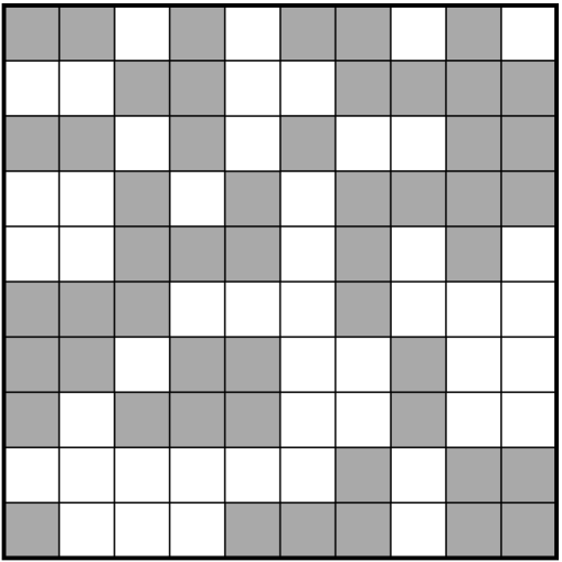
Figure 10: The percolation model on a square lattice: squares on the lattice are coloured in independently at random with some probability $p$. In this example $p=\mbox{$\frac{1}{2}$}$.

When $p$ is small, only a few squares are coloured in and most coloured squares will be alone on the lattice, or maybe grouped in twos or threes. So $\left\langle s\right\rangle$ will be small. This situation is depicted in Fig. 11 for $p=0.3$. Conversely, if $p$ is large—almost 1, which is the largest value it can have—then most squares will be coloured in and they will almost all be connected together in one large cluster, the so-called spanning cluster. In this situation we say that the system percolates. Now the mean size of the cluster to which a vertex belongs is limited only by the size of the lattice itself and as we let the lattice size become large $\left\langle s\right\rangle$ also becomes large. So we have two distinctly different behaviours, one for small $p$ in which $\left\langle s\right\rangle$ is small and doesn’t depend on the size of the system, and one for large $p$ in which $\left\langle s\right\rangle$ is much larger and increases with the size of the system.

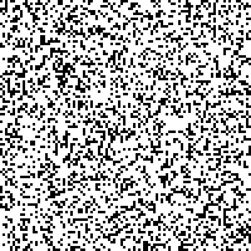
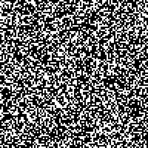
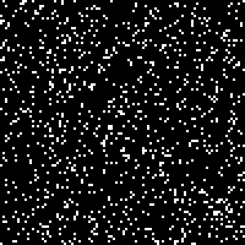
Figure 11: Three examples of percolation systems on $100\times 100$ square lattices with $p=0.3$, $p=p_{c}=0.5927\ldots$ and $p=0.9$. The first and last are well below and above the critical point respectively, while the middle example is precisely at it.

And what happens in between these two extremes? As we increase $p$ from small values, the value of $\left\langle s\right\rangle$ also increases. But at some point we reach the start of the regime in which $\left\langle s\right\rangle$ goes up with system size instead of staying constant. We now know that this point is at $p=0.5927462\ldots$, which is called the critical value of $p$ and is denoted $p_{c}$. If the size of the lattice is large, then $\left\langle s\right\rangle$ also becomes large at this point, and in the limit where the lattice size goes to infinity $\left\langle s\right\rangle$ actually diverges. To illustrate this phenomenon, I show in Fig. 12 a plot of $\left\langle s\right\rangle$ from simulations of the percolation model and the divergence is clear.

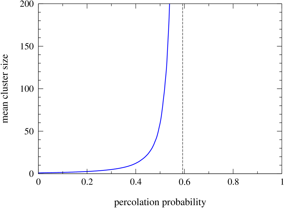
Figure 12: The mean area of the cluster to which a randomly chosen square belongs for the percolation model described in the text, calculated from an average over 1000 simulations on a $1000\times 1000$ square lattice. The dotted line marks the known position of the phase transition.

Now consider not just the mean cluster size but the entire distribution of cluster sizes. Let $p(s)$ be the probability that a randomly chosen square belongs to a cluster of area $s$. In general, what forms can $p(s)$ take as a function of $s$? The important point to notice is that $p(s)$, being a probability distribution, is a dimensionless quantity—just a number—but $s$ is an area. We could measure $s$ in terms of square metres, or whatever units the lattice is calibrated in. The average $\left\langle s\right\rangle$ is also an area and then there is the area of a unit square itself, which we will denote $a$. Other than these three quantities, however, there are no other independent parameters with dimensions in this problem. (There is the area of the whole lattice, but we are considering the limit where that becomes infinite, so it’s out of the picture.)

If we want to make a dimensionless function $p(s)$ out of these three dimensionful parameters, there are three dimensionless ratios we can form: $s/a$, $a/\left\langle s\right\rangle$ and $s/\left\langle s\right\rangle$ (or their reciprocals, if we prefer). Only two of these are independent however, since the last is the product of the other two. Thus in general we can write

$$p(s)=Cf\biggl{(}{s\over a},{a\over\left\langle s\right\rangle}\biggr{)},$$ (78)

where $f$ is a dimensionless mathematical function of its dimensionless arguments and $C$ is a normalizing constant chosen so that $\sum_{s}p(s)=1$.

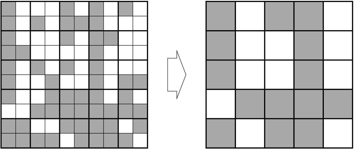
Figure 13: A site percolation system is coarse-grained, so that the area of the fundamental square is (in this case) quadrupled. The occupation of the squares in the coarse-grained lattice (right) is chosen to mirror as nearly as possible that of the squares on the original lattice (left), so that the sizes and shapes of the large clusters remain roughly the same. The small clusters are mostly lost in the coarse-graining, so that the arguments given in the text are valid only for the large-$s$ tail of the cluster size distribution.

But now here’s the trick. We can coarse-grain or rescale our lattice so that the fundamental unit of the lattice changes. For instance, we could double the size of our unit square $a$. The kind of picture I’m thinking of is shown in Fig. 13. The basic percolation clusters stay roughly the same size and shape, although I’ve had to fudge things around the edges a bit to make it work. For this reason this argument will only be strictly correct for large clusters $s$ whose area is not changed appreciably by the fudging. (And the argument thus only tells us that the tail of the distribution is a power law, and not the whole distribution.)

The probability $p(s)$ of getting a cluster of area $s$ is unchanged by the coarse-graining since the areas themselves are, to a good approximation, unchanged, and the mean cluster size is thus also unchanged. All that has changed, mathematically speaking, is that the unit area $a$ has been rescaled $a\to a/b$ for some constant rescaling factor $b$. The equivalent of Eq. (78) in our coarse-grained system is

$$p(s)=C^{\prime}f\biggl{(}{s\over a/b},{a/b\over\left\langle s\right\rangle}\biggr{)}=C^{\prime}f\biggl{(}{bs\over a},{a\over b\left\langle s\right\rangle}\biggr{)}.$$ (79)

Comparing with Eq. (78), we can see that this is equal, to within a multiplicative constant, to the probability $p(bs)$ of getting a cluster of size $bs$, but in a system with a different mean cluster size of $b\left\langle s\right\rangle$. Thus we have related the probabilities of two different sizes of clusters to one another, but on systems with different average cluster size and hence presumably also different site occupation probability. Note that the normalization constant must in general be changed in Eq. (79) to make sure that $p(s)$ still sums to unity, and that this change will depend on the value we choose for the rescaling factor $b$.

But now we notice that there is one special point at which this rescaling by definition does not result in a change in $\left\langle s\right\rangle$ or a corresponding change in the site occupation probability, and that is the critical point. When we are precisely at the point at which $\left\langle s\right\rangle\to\infty$, then $b\left\langle s\right\rangle=\left\langle s\right\rangle$ by definition. Putting $\left\langle s\right\rangle\to\infty$ in Eqs. (78) and (79), we then get $p(s)=C^{\prime}f({bs/a},0)=(C^{\prime}/C)p(bs)$. Or equivalently

$$p(bs)=g(b)p(s),$$ (80)

where $g(b)=C/C^{\prime}$. Comparing with Eq. (29) we see that this has precisely the form of the equation that defines a scale-free distribution. The rest of the derivation below Eq. (29) follows immediately, and so we know that $p(s)$ must follow a power law.

This in fact is the origin of the name “scale-free” for a distribution of the form (29). At the point at which $\left\langle s\right\rangle$ diverges, the system is left with no defining size-scale, other than the unit of area $a$ itself. It is “scale-free”, and by the argument above it follows that the distribution of $s$ must obey a power law.

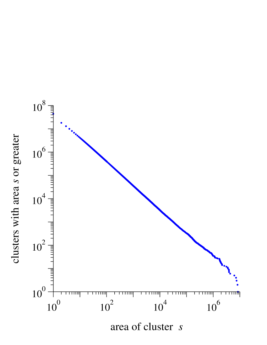
Figure 14: Cumulative distribution of the sizes of clusters for (site) percolation on a square lattice of $40\,000\times 40\,000$ sites at the critical site occupation probability $p_{c}=0.592746\ldots$

In Fig. 14 I show an example of a cumulative distribution of cluster sizes for a percolation system right at the critical point and, as the figure shows, the distribution does indeed follow a power law. Technically the distribution cannot follow a power law to arbitrarily large cluster sizes since the area of a cluster can be no bigger than the area of the whole lattice, so the power-law distribution will be cut off in the tail. This is an example of a finite-size effect. This point does not seem to be visible in Fig. 14 however.

The kinds of arguments given in this section can be made more precise using the machinery of the renormalization group. The real-space renormalization group makes use precisely of transformations such as that shown in Fig. 13 to derive power-law forms and their exponents for distributions at the critical point. An example application to the percolation problem is given by Reynolds et al. [55]. A more technically sophisticated technique is the $k$-space renormalization group, which makes use of transformations in Fourier space to accomplish similar aims in a particularly elegant formal environment [56].

IV.6 Self-organized criticality

As discussed in the preceding section, certain systems develop power-law distributions at special “critical” points in their parameter space because of the divergence of some characteristic scale, such as the mean cluster size in the percolation model. This does not, however, provide a plausible explanation for the origin of power laws in most real systems. Even if we could come up with some model of earthquakes or solar flares or web hits that had such a divergence, it seems unlikely that the parameters of the real world would, just coincidentally, fall precisely at the point where the divergence occurred.

As first proposed by Bak et al. [57], however, it is possible that some dynamical systems actually arrange themselves so that they always sit at the critical point, no matter what state we start off in. One says that such systems self-organize to the critical point, or that they display self-organized criticality. A now-classic example of such a system is the forest fire model of Drossel and Schwabl [58], which is based on the percolation model we have already seen.

Consider the percolation model as a primitive model of a forest. The lattice represents the landscape and a single tree can grow in each square. Occupied squares represent trees and empty squares represent empty plots of land with no trees. Trees appear instantaneously at random at some constant rate and hence the squares of the lattice fill up at random. Every once in a while a wildfire starts at a random square on the lattice, set off by a lightning strike perhaps, and burns the tree in that square, if there is one, along with every other tree in the cluster connected to it. The process is illustrated in Fig. 15. One can think of the fire as leaping from tree to adjacent tree until the whole cluster is burned, but the fire cannot cross the firebreak formed by an empty square. If there is no tree in the square struck by the lightning, then nothing happens. After a fire, trees can grow up again in the squares vacated by burnt trees, so the process keeps going indefinitely.

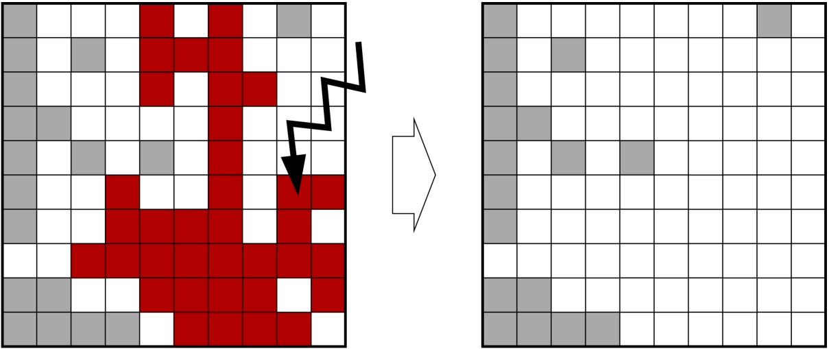
Figure 15: Lightning strikes at random positions in the forest fire model, starting fires that wipe out the entire cluster to which a struck tree belongs.

If we start with an empty lattice, trees will start to appear but will initially be sparse and lightning strikes will either hit empty squares or if they do chance upon a tree they will burn it and its cluster, but that cluster will be small and localized because we are well below the percolation threshold. Thus fires will have essentially no effect on the forest. As time goes by however, more and more trees will grow up until at some point there are enough that we have percolation. At that point, as we have seen, a spanning cluster forms whose size is limited only by the size of the lattice, and when any tree in that cluster gets hit by the lightning the entire cluster will burn away. This gets rid of the spanning cluster so that the system does not percolate any more, but over time as more trees appear it will presumably reach percolation again, and so the scenario will play out repeatedly. The end result is that the system oscillates right around the critical point, first going just above the percolation threshold as trees appear and then being beaten back below it by fire. In the limit of large system size these fluctuations become small compared to the size of the system as a whole and to an excellent approximation the system just sits at the threshold indefinitely. Thus, if we wait long enough, we expect the forest fire model to self-organize to a state in which it has a power-law distribution of the sizes of clusters, or of the sizes of fires.

In Fig. 16 I show the cumulative distribution of the sizes of fires in the forest fire model and, as we can see, it follows a power law closely. The exponent of the distribution is quite small in this case. The best current estimates give a value of $\alpha=1.19\pm 0.01$ [59], meaning that the distribution has an infinite mean in the limit of large system size. For all real systems however the mean is finite: the distribution is cut off in the large-size tail because fires cannot have a size any greater than that of the lattice as a whole and this makes the mean well-behaved. This cutoff is clearly visible in Fig. 16 as the drop in the curve towards the right of the plot. What’s more the distribution of the sizes of fires in real forests, Fig. 5d, shows a similar cutoff and is in many ways qualitatively similar to the distribution predicted by the model. (Real forests are obviously vastly more complex than the forest fire model, and no one is seriously suggesting that the model is an accurate representation the real world. Rather it is a guide to the general type of processes that might be going on in forests.)

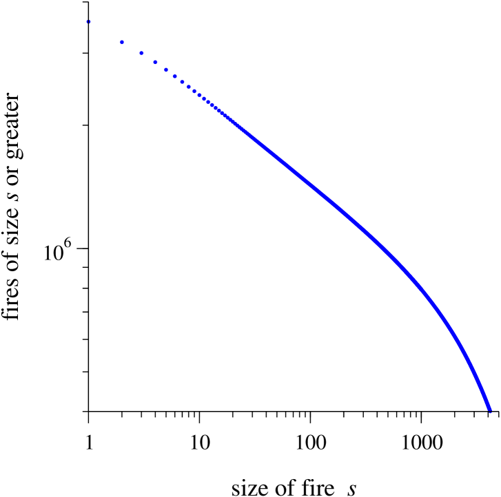
Figure 16: Cumulative distribution of the sizes of “fires” in a simulation of the forest fire model of Drossel and Schwabl [58] for a square lattice of size $5000\times 5000$.

There has been much excitement about self-organized criticality as a possible generic mechanism for explaining where power-law distributions come from. Per Bak, one of the originators of the idea, wrote an entire book about it [60]. Self-organized critical models have been put forward not only for forest fires, but for earthquakes [61, 62], solar flares [5], biological evolution [63], avalanches [57] and many other phenomena. Although it is probably not the universal law that some have claimed it to be, it is certainly a powerful and intriguing concept that potentially has applications to a variety of natural and man-made systems.

IV.7 Other mechanisms for generating power laws

In the preceding sections I’ve described the best known and most widely applied mechanisms that generate power-law distributions. However, there are a number of others that deserve a mention. One that has been receiving some attention recently is the highly optimized tolerance mechanism of Carlson and Doyle [64, 65]. The classic example of this mechanism is again a model of forest fires and is based on the percolation process. Suppose again that fires start at random in a grid-like forest, just as we considered in Sec. IV.6, but suppose now that instead of appearing at random, trees are deliberately planted by a knowledgeable forester. One can ask what the best distribution of trees is to optimize the amount of lumber the forest produces, subject to random fires that could start at any place. The answer turns out to be that one should plant trees in blocks, with narrow firebreaks between them to prevent fires from spreading. Moreover, one should make the blocks smaller in regions where fires start more often and larger where fires are rare. The reason for this is that we waste some valuable space by making firebreaks, space in which we could have planted more trees. If fires are rare, then on average it pays to put the breaks further apart—more trees will burn if there is a fire, but we also get more lumber if there isn’t.

Carlson and Doyle show both by analytic arguments and by numerical simulation that for quite general distributions of starting points for fires this process leads to a distribution of fire sizes that approximately follows a power law. The distribution is not a perfect power law in this case, but on the other hand neither are many of those seen in the data of Fig. 4, so this is not necessarily a disadvantage. Carlson and Doyle have proposed that highly optimized tolerance could be a model not only for forest fires but also for the sizes of files on the world wide web, which appear to follow a power law [6].

Another mechanism, which is mathematically similar to that of Carlson and Doyle but quite different in motivation, is the coherent noise mechanism proposed by Sneppen and Newman [66] as a model of biological extinction. In this mechanism a number of agents or species are subjected to stresses of various sizes, and each agent has a threshold for stress above which an applied stress will wipe that agent out—the species becomes extinct. Extinct species are replaced by new ones with randomly chosen thresholds. The net result is that the system self-organizes to a state where most of the surviving species have high thresholds, but the exact distribution depends on the distribution of stresses in a way very similar to the relation between block sizes and fire frequency in highly optimized tolerance. No conscious optimization is needed in this case, but the end result is similar: the overall distribution of the numbers of species becoming extinct as a result of any particular stress approximately follows a power law. The power-law form is not exact, but it’s as good as that seen in real extinction data. Sneppen and Newman have also suggested that their mechanism could be used to model avalanches and earthquakes.

One of the broad distributions mentioned in Sec. II.2 as an alternative to the power law was the log-normal. A log-normally distributed quantity is one whose logarithm is normally distributed. That is

$$p(\ln x)\sim\exp\biggl{(}-{(\ln x-\mu)^{2}\over 2\sigma^{2}}\biggr{)},$$ (81)

for some choice of the mean $\mu$ and standard deviation $\sigma$ of the distribution. Distributions like this typically arise when we are multiplying together random numbers. The log of the product of a large number of random numbers is the sum of the logarithms of those same random numbers, and by the central limit theorem such sums have a normal distribution essentially regardless of the distribution of the individual numbers.

But Eq. (81) implies that the distribution of $x$ itself is

$$p(x)=p(\ln x){{\rm d}\ln x\over{\rm d}x}={1\over x}\exp\biggl{(}-{(\ln x-\mu)^{2}\over 2\sigma^{2}}\biggr{)}.$$ (82)

To see how this looks if we were to plot it on log scales, we take logarithms of both sides, giving

$$\ln p(x) = -\ln x-{(\ln x-\mu)^{2}\over 2\sigma^{2}}$$ (83)

$$= -{(\ln x)^{2}\over 2\sigma^{2}}+\biggl{[}{\mu\over\sigma^{2}}-1\biggr{]}\ln x-{\mu^{2}\over 2\sigma^{2}},$$

which is quadratic in $\ln x$. However, any quadratic curve looks straight if we view a sufficient small portion of it, so $p(x)$ will look like a power-law distribution when we look at a small portion on log scales. The effective exponent $\alpha$ of the distribution is in this case not fixed by the theory—it could be anything, depending on which part of the quadratic our data fall on.

On larger scales the distribution will have some downward curvature, but so do many of the distributions claimed to follow power laws, so it is possible that these distributions are really log-normal. In fact, in many cases we don’t even have to restrict ourselves to a particularly small a portion of the curve. If $\sigma$ is large then the quadratic term in Eq. (83) will vary slowly and the curvature of the line will be slight, so the distribution will appear to follow a power law over relatively large portions of its range. This situation arises commonly when we are considering products of random numbers.

Suppose for example that we are multiplying together 100 numbers, each of which is drawn from some distribution such that the standard deviation of the logs is around 1—i.e., the numbers themselves vary up or down by about a factor of ${\rm e}$. Then, by the central limit theorem, the standard deviation for $\ln x$ will be $\sigma\simeq 10$ and $\ln x$ will have to vary by about $\pm 10$ for changes in $(\ln x)^{2}/\sigma^{2}$ to be apparent. But such a variation in the logarithm corresponds to a variation in $x$ of more than four orders of magnitude. If our data span a domain smaller than this, as many of the plots in Fig. 4 do, then we will see a measured distribution that looks close to power-law. And the range will get quickly larger as the number of numbers we are multiplying grows.

One example of a random multiplicative process might be wealth generation by investment. If a person invests money, for instance in the stock market, they will get a percentage return on their investment that varies over time. In other words, in each period of time their investment is multiplied by some factor which fluctuates from one period to the next. If the fluctuations are random and uncorrelated, then after many such periods the value of the investment is the initial value multiplied by the product of a large number of random numbers, and therefore should be distributed according to a log-normal. This could explain why the tail of the wealth distribution, Fig. 4j, appears to follow a power law.

Another example is fragmentation. Suppose we break a stick of unit length into two parts at a position which is a random fraction $z$ of the way along the stick’s length. Then we break the resulting pieces at random again and so on. After many breaks, the length of one of the remaining pieces will be $\prod_{i}z_{i}$, where $z_{i}$ is the position of the $i$th break. This is a product of random numbers and thus the resulting distribution of lengths should follow a power law over a portion of its range. A mechanism like this could, for instance, produce a power-law distribution of meteors or other interplanetary rock fragments, which tend to break up when they collide with one another, and this in turn could produce a power-law distribution of the sizes of meteor craters similar to the one in Fig. 4g.

In fact, as discussed by a number of authors [67, 68, 69], random multiplication processes can also generate perfect power-law distributions with only a slight modification: if there is a lower bound on the value that the product of a set of numbers is allowed to take (for example if there is a “reflecting boundary” on the lower end of the range, or an additive noise term as well as a multiplicative one) then the behaviour of the process is modified to generate not a log-normal, but a true power law.

Finally, some processes show power-law distributions of times between events. The distribution of times between earthquakes and their aftershocks is one example. Such power-law distributions of times are observed in critical models and in the coherent noise mechanism mentioned above, but another possible explanation for their occurrence is a random extremal process or record dynamics. In this mechanism we consider how often a randomly fluctuating quantity will break its own record for the highest value recorded. For a quantity with, say, a Gaussian distribution, it is always in theory possible for the record to be broken, no matter what its current value, but the more often the record is broken the higher the record will get and the longer we will have to wait until it is broken again. As shown by Sibani and Littlewood [70], this non-stationary process gives a distribution of waiting times between the establishment of new records that follows a power law with exponent $\alpha=1$. Interestingly, this is precisely the exponent observed for the distribution of waiting times for aftershocks of earthquakes. The record dynamics has also been proposed as a model for the lifetimes of biological taxa [71].

V Conclusions

In this review I have discussed the power-law statistical distributions seen in a wide variety of natural and man-made phenomena, from earthquakes and solar flares to populations of cities and sales of books. We have seen many examples of power-law distributions in real data and seen how to analyse those data to understand the behaviour and parameters of the distributions. I have also described a number of physical mechanisms that have been proposed to explain the occurrence of power laws. Perhaps the two most important of these are:

1. The Yule process, a rich-get-richer mechanism in which the most populous cities or best-selling books get more inhabitants or sales in proportion to the number they already have. Yule and later Simon showed mathematically that this mechanism produces what is now called the Yule distribution, which follows a power law in its tail.

2. Critical phenomena and the associated concept of self-organized criticality, in which a scale-factor of a system diverges, either because we have tuned the system to a special critical point in its parameter space or because the system automatically drives itself to that point by some dynamical process. The divergence can leave the system with no appropriate scale factor to set the size of some measured quantity and as we have seen the quantity must then follow a power law.

The study of power-law distributions is an area in which there is considerable current research interest. While the mechanisms and explanations presented here certainly offer some insight, there is much work to be done both experimentally and theoretically before we can say we really understand the physical processes driving these systems. Without doubt there are many exciting discoveries still waiting to be made.

Appendix A Rank/frequency plots

Suppose we wish to make a plot of the cumulative distribution function $P(x)$ of a quantity such as, for example, the frequency with which words appear in a body of text (Fig. 4a). We start by making a list of all the words along with their frequency of occurrence. Now the cumulative distribution of the frequency is defined such that $P(x)$ is the fraction of words with frequency greater than or equal to $x$. Or alternatively one could simply plot the number of words with frequency greater than or equal to $x$, which differs from the fraction only in its normalization.

Now consider the most frequent word, which is “the” in most written English texts. If $x$ is the frequency with which this word occurs, then clearly there is exactly one word with frequency greater than or equal to $x$, since no other word is more frequent. Similarly, for the frequency of the second most common word—usually “of”—there are two words with that frequency or greater, namely “of” and “the”. And so forth. In other words, if we rank the words in order, then by definition there are $n$ words with frequency greater than or equal to that of the $n$th most common word. Thus the cumulative distribution $P(x)$ is simply proportional to the rank $n$ of a word. This means that to make a plot of $P(x)$ all we need do is sort the words in decreasing order of frequency, number them starting from 1, and then plot their ranks as a function of their frequency. Such a plot of rank against frequency was called by Zipf [2] a rank/frequency plot, and this name is still sometimes used to refer to plots of the cumulative distribution of a quantity. Of course, many quantities we are interested in are not frequencies—they are the sizes of earthquakes or people’s personal wealth or whatever—but nonetheless people still talk about “rank/frequency” plots although the name is not technically accurate.

In practice, sorting and ranking measurements and then plotting rank against those measurements is usually the quickest way to construct a plot of the cumulative distribution of a quantity. All the cumulative plots in this paper were made in this way, except for the plot of the sizes of moon craters in Fig. 4g, for which the data came already in cumulative form.

Appendix B Maximum likelihood estimate of exponents

Consider the power-law distribution

$$p(x)=Cx^{-\alpha}={\alpha-1\over x_{\mathrm{min}}}\biggl{(}{x\over x_{\mathrm{min}}}\biggr{)}^{-\alpha},$$ (84)

where we have made use of the value of the normalization constant $C$ calculated in Eq. (9).

Given a set of $n$ values $x_{i}$, the probability that those values were generated from this distribution is proportional to

$$P(x|\alpha)=\prod_{i=1}^{n}p(x_{i})=\prod_{i=1}^{n}{\alpha-1\over x_{\mathrm{min}}}\biggl{(}{x_{i}\over x_{\mathrm{min}}}\biggr{)}^{-\alpha}.$$ (85)

This quantity is called the likelihood of the data set.

To find the value of $\alpha$ that best fits the data, we need to calculate the probability $P(\alpha|x)$ of a particular value of $\alpha$ given the observed $\{x_{i}\}$, which is related to $P(x|\alpha)$ by Bayes’ law thus:

$$P(\alpha|x)=P(x|\alpha){P(\alpha)\over P(x)}.$$ (86)

The prior probability of the data $P(x)$ is fixed since $x$ itself is fixed—$x$ is equal to the particular set of observations we actually made and does not vary in the calculation—and it is usually assumed, in the absence of any information to the contrary, that the prior probability of the exponent $P(\alpha)$ is uniform, i.e., a constant independent of $\alpha$. Thus $P(\alpha|x)\propto P(x|\alpha)$. For convenience we typically work with the logarithm of $P(\alpha|x)$, which, to within an additive constant, is equal to the log of the likelihood, denoted $\mathcal{L}$ and given by

$$\mathcal{L} = \ln P(x|\alpha)=\sum_{i=1}^{n}\biggl{[}\ln(\alpha-1)-\ln x_{\mathrm{min}}-\alpha\ln{x_{i}\over x_{\mathrm{min}}}\biggr{]}$$ (87)

$$= n\ln(\alpha-1)-n\ln x_{\mathrm{min}}-\alpha\sum_{i=1}^{n}\ln{x_{i}\over x_{\mathrm{min}}}.$$

Now we calculate the most likely value of $\alpha$ by maximizing the likelihood with respect to $\alpha$, which is the same as maximizing the log likelihood, since the logarithm is a monotonic increasing function. Setting $\partial\mathcal{L}/\partial\alpha=0$, we find

$${n\over\alpha-1}-\sum_{i=1}^{n}\ln{x_{i}\over x_{\mathrm{min}}}=0,$$ (88)

or

$$\alpha=1+n\biggl{[}\sum_{i}\ln{x_{i}\over x_{\mathrm{min}}}\biggr{]}^{-1}.$$ (89)

We also wish to know what the expected error is on our value of $\alpha$. We can estimate this from the width of the maximum of the likelihood as a function of $\alpha$. Taking the exponential of Eq. (87), we find that that the likelihood has the form

$$P(x|\alpha)=a{\rm e}^{-b\alpha}(\alpha-1)^{n},$$ (90)

where $b=\sum_{i=1}^{n}\ln(x_{i}/x_{\mathrm{min}})$ and $a$ is an unimportant normalizing constant. Assuming that $\alpha>1$ so that the distribution (84) is normalizable, the mean and mean square of $\alpha$ in this distribution are given by

$$\left\langle\alpha\right\rangle = {\int_{1}^{\infty}{\rm e}^{-b\alpha}(\alpha-1)^{n}\alpha\>{\rm d}\alpha\over\int_{1}^{\infty}{\rm e}^{-b\alpha}(\alpha-1)^{n}\>{\rm d}\alpha}$$ (91)

$$= {{\rm e}^{-b}b^{-2-n}(n+1+b)\Gamma(n+1)\over{\rm e}^{-b}b^{-1-n}\Gamma(n+1)}$$

$$= {n+1+b\over b}$$

and

$$\left\langle\alpha^{2}\right\rangle = {\int_{1}^{\infty}{\rm e}^{-b\alpha}(\alpha-1)^{n}\alpha^{2}\>{\rm d}\alpha\over\int_{1}^{\infty}{\rm e}^{-b\alpha}(\alpha-1)^{n}\>{\rm d}\alpha}$$ (92)

$$= {{\rm e}^{-b}b^{-3-n}(n^{2}+3n+b^{2}+2b+2nb+2)\Gamma(n+1)\over{\rm e}^{-b}b^{-1-n}\Gamma(n+1)}$$

$$= {n^{2}+3n+b^{2}+2b+2nb+2\over b^{2}},$$

where $\Gamma(x)$ is the $\Gamma$-function of Eq. (21). Then the variance of $\alpha$ is

$$\sigma^{2} = \left\langle\alpha^{2}\right\rangle-\left\langle\alpha\right\rangle^{2}$$ (93)

$$= {n^{2}+3n+b^{2}+2b+2nb+2\over b^{2}}-{(n+1+b)^{2}\over b^{2}}$$

$$= {n+1\over b^{2}},$$

and the error on $\alpha$ is

$$\sigma={\sqrt{n+1}\over b}=\sqrt{n+1}\biggl{[}\sum_{i}\ln{x_{i}\over x_{\mathrm{min}}}\biggr{]}^{-1}.$$ (94)

In most cases we will have $n\gg 1$ and it is safe to approximate $n+1$ by $n$, giving

$$\sigma=\sqrt{n}\biggl{[}\sum_{i}\ln{x_{i}\over x_{\mathrm{min}}}\biggr{]}^{-1}={\alpha-1\over\sqrt{n}},$$ (95)

where $\alpha$ in this expression is the maximum likelihood estimate from Eq. (89).

References

- [1] F. Auerbach, Das Gesetz der Bevölkerungskonzentration. Petermanns Geographische Mitteilungen 59, 74–76 (1913).
- [2] G. K. Zipf, Human Behaviour and the Principle of Least Effort. Addison-Wesley, Reading, MA (1949).
- [3] B. Gutenberg and R. F. Richter, Frequency of earthquakes in california. Bulletin of the Seismological Society of America 34, 185–188 (1944).
- [4] G. Neukum and B. A. Ivanov, Crater size distributions and impact probabilities on Earth from lunar, terrestial-planet, and asteroid cratering data. In T. Gehrels (ed.), Hazards Due to Comets and Asteroids, pp. 359–416, University of Arizona Press, Tucson, AZ (1994).
- [5] E. T. Lu and R. J. Hamilton, Avalanches of the distribution of solar flares. Astrophysical Journal 380, 89–92 (1991).
- [6] M. E. Crovella and A. Bestavros, Self-similarity in World Wide Web traffic: Evidence and possible causes. In B. E. Gaither and D. A. Reed (eds.), Proceedings of the 1996 ACM SIGMETRICS Conference on Measurement and Modeling of Computer Systems, pp. 148–159, Association of Computing Machinery, New York (1996).
- [7] D. C. Roberts and D. L. Turcotte, Fractality and self-organized criticality of wars. Fractals 6, 351–357 (1998).
- [8] J. B. Estoup, Gammes Stenographiques. Institut Stenographique de France, Paris (1916).
- [9] D. H. Zanette and S. C. Manrubia, Vertical transmission of culture and the distribution of family names. Physica A 295, 1–8 (2001).
- [10] A. J. Lotka, The frequency distribution of scientific production. J. Wash. Acad. Sci. 16, 317–323 (1926).
- [11] D. J. de S. Price, Networks of scientific papers. Science 149, 510–515 (1965).
- [12] L. A. Adamic and B. A. Huberman, The nature of markets in the World Wide Web. Quarterly Journal of Electronic Commerce 1, 512 (2000).
- [13] R. A. K. Cox, J. M. Felton, and K. C. Chung, The concentration of commercial success in popular music: an analysis of the distribution of gold records. Journal of Cultural Economics 19, 333–340 (1995).
- [14] R. Kohli and R. Sah, Market shares: Some power law results and observations. Working paper 04.01, Harris School of Public Policy, University of Chicago (2003).
- [15] J. C. Willis and G. U. Yule, Some statistics of evolution and geographical distribution in plants and animals, and their significance. Nature 109, 177–179 (1922).
- [16] V. Pareto, Cours d’Economie Politique. Droz, Geneva (1896).
- [17] G. B. West, J. H. Brown, and B. J. Enquist, A general model for the origin of allometric scaling laws in biology. Science 276, 122–126 (1997).
- [18] D. Sornette, Critical Phenomena in Natural Sciences, chapter 14. Springer, Heidelberg, 2nd edition (2003).
- [19] M. Mitzenmacher, A brief history of generative models for power law and lognormal distributions. Internet Mathematics 1, 226–251 (2004).
- [20] M. L. Goldstein, S. A. Morris, and G. G. Yen, Problems with fitting to the power-law distribution. Eur. Phys. J. B 41, 255–258 (2004).
- [21] H. Dahl, Word Frequencies of Spoken American English. Verbatim, Essex, CT (1979).
- [22] S. Redner, How popular is your paper? An empirical study of the citation distribution. Eur. Phys. J. B 4, 131–134 (1998).
- [23] A. P. Hackett, 70 Years of Best Sellers, 1895-1965. R. R. Bowker Company, New York, NY (1967).
- [24] W. Aiello, F. Chung, and L. Lu, A random graph model for massive graphs. In Proceedings of the 32nd Annual ACM Symposium on Theory of Computing, pp. 171–180, Association of Computing Machinery, New York (2000).
- [25] H. Ebel, L.-I. Mielsch, and S. Bornholdt, Scale-free topology of e-mail networks. Phys. Rev. E 66, 035103 (2002).
- [26] B. A. Huberman and L. A. Adamic, Information dynamics in the networked world. In E. Ben-Naim, H. Frauenfelder, and Z. Toroczkai (eds.), Complex Networks, number 650 in Lecture Notes in Physics, pp. 371–398, Springer, Berlin (2004).
- [27] M. Small and J. D. Singer, Resort to Arms: International and Civil Wars, 1816-1980. Sage Publications, Beverley Hills (1982).
- [28] S. Miyazima, Y. Lee, T. Nagamine, and H. Miyajima, Power-law distribution of family names in Japanese societies. Physica A 278, 282–288 (2000).
- [29] B. J. Kim and S. M. Park, Distribution of Korean family names. Preprint cond-mat/0407311 (2004).
- [30] J. Chen, J. S. Thorp, and M. Parashar, Analysis of electric power disturbance data. In 34th Hawaii International Conference on System Sciences, IEEE Computer Society (2001).
- [31] B. A. Carreras, D. E. Newman, I. Dobson, and A. B. Poole, Evidence for self-organized criticality in electric power system blackouts. In 34th Hawaii International Conference on System Sciences, IEEE Computer Society (2001).
- [32] E. Limpert, W. A. Stahel, and M. Abbt, Log-normal distributions across the sciences: Keys and clues. Bioscience 51, 341–352 (2001).
- [33] M. E. J. Newman, S. Forrest, and J. Balthrop, Email networks and the spread of computer viruses. Phys. Rev. E 66, 035101 (2002).
- [34] M. O. Lorenz, Methods of measuring the concentration of wealth. Publications of the American Statisical Association 9, 209–219 (1905).
- [35] H. A. Simon, On a class of skew distribution functions. Biometrika 42, 425–440 (1955).
- [36] G. U. Yule, A mathematical theory of evolution based on the conclusions of Dr. J. C. Willis. Philos. Trans. R. Soc. London B 213, 21–87 (1925).
- [37] G. A. Miller, Some effects of intermittent silence. American Journal of Psychology 70, 311–314 (1957).
- [38] W. Li, Random texts exhibit Zipf’s-law-like word frequency distribution. IEEE Transactions on Information Theory 38, 1842–1845 (1992).
- [39] C. E. Shannon, A mathematical theory of communication I. Bell System Technical Journal 27, 379–423 (1948).
- [40] C. E. Shannon, A mathematical theory of communication II. Bell System Technical Journal 27, 623–656 (1948).
- [41] T. M. Cover and J. A. Thomas, Elements of Information Theory. John Wiley, New York (1991).
- [42] B. B. Mandelbrot, An information theory of the statsitical structure of languages. In W. Jackson (ed.), Symp. Applied Communications Theory, pp. 486–502, Butterworth, Woburn, MA (1953).
- [43] W. J. Reed and B. D. Hughes, From gene families and genera to incomes and internet file sizes: Why power laws are so common in nature. Phys. Rev. E 66, 067103 (2002).
- [44] J.-P. Bouchaud, More Lévy distributions in physics. In M. F. Shlesinger, G. M. Zaslavsky, and U. Frisch (eds.), Lévy Flights and Related Topics in Physics, number 450 in Lecture Notes in Physics, Springer, Berlin (1995).
- [45] N. Jan, L. Moseley, T. Ray, and D. Stauffer, Is the fossil record indicative of a critical system? Adv. Complex Syst. 2, 137–141 (1999).
- [46] D. Sornette, Mechanism for powerlaws without self-organization. Int. J. Mod. Phys. C 13, 133–136 (2001).
- [47] R. H. Swendsen and J.-S. Wang, Nonuniversal critical dynamics in Monte Carlo simulations. Phys. Rev. Lett. 58, 86–88 (1987).
- [48] K. Sneppen, P. Bak, H. Flyvbjerg, and M. H. Jensen, Evolution as a self-organized critical phenomenon. Proc. Natl. Acad. Sci. USA 92, 5209–5213 (1995).
- [49] M. E. J. Newman and R. G. Palmer, Modeling Extinction. Oxford University Press, Oxford (2003).
- [50] D. J. de S. Price, A general theory of bibliometric and other cumulative advantage processes. J. Amer. Soc. Inform. Sci. 27, 292–306 (1976).
- [51] P. L. Krapivsky, S. Redner, and F. Leyvraz, Connectivity of growing random networks. Phys. Rev. Lett. 85, 4629–4632 (2000).
- [52] A.-L. Barabási and R. Albert, Emergence of scaling in random networks. Science 286, 509–512 (1999).
- [53] S. N. Dorogovtsev, J. F. F. Mendes, and A. N. Samukhin, Structure of growing networks with preferential linking. Phys. Rev. Lett. 85, 4633–4636 (2000).
- [54] R. K. Merton, The Matthew effect in science. Science 159, 56–63 (1968).
- [55] P. J. Reynolds, W. Klein, and H. E. Stanley, A real-space renormalization group for site and bond percolation. J. Phys. C 10, L167–L172 (1977).
- [56] K. G. Wilson and J. Kogut, The renormalization group and the -expansion. Physics Reports 12, 75–199 (1974).
- [57] P. Bak, C. Tang, and K. Wiesenfeld, Self-organized criticality: An explanation of the 1/f noise. Phys. Rev. Lett. 59, 381–384 (1987).
- [58] B. Drossel and F. Schwabl, Self-organized critical forest-fire model. Phys. Rev. Lett. 69, 1629–1632 (1992).
- [59] P. Grassberger, Critical behaviour of the drossel-schwabl forest fire model. New Journal of Physics 4, 17 (2002).
- [60] P. Bak, How Nature Works: The Science of Self-Organized Criticality. Copernicus, New York (1996).
- [61] P. Bak and C. Tang, Earthquakes as a self-organized critical phenomenon. Journal of Geophysical Research 94, 15635–15637 (1989).
- [62] Z. Olami, H. J. S. Feder, and K. Christensen, Self-organized criticality in a continuous, nonconservative cellular automaton modeling earthquakes. Phys. Rev. Lett. 68, 1244–1247 (1992).
- [63] P. Bak and K. Sneppen, Punctuated equilibrium and criticality in a simple model of evolution. Phys. Rev. Lett. 74, 4083–4086 (1993).
- [64] J. M. Carlson and J. Doyle, Highly optimized tolerance: A mechanism for power laws in designed systems. Phys. Rev. E 60, 1412–1427 (1999).
- [65] J. M. Carlson and J. Doyle, Highly optimized tolerance: Robustness and design in complex systems. Phys. Rev. Lett. 84, 2529–2532 (2000).
- [66] K. Sneppen and M. E. J. Newman, Coherent noise, scale invariance and intermittency in large systems. Physica D 110, 209–222 (1997).
- [67] D. Sornette and R. Cont, Convergent multiplicative processes repelled from zero: Power laws and truncated power laws. Journal de Physique I 7, 431–444 (1997).
- [68] D. Sornette, Multiplicative processes and power laws. Phys. Rev. E 57, 4811–4813 (1998).
- [69] X. Gabaix, Zipf’s law for cities: An explanation. Quarterly Journal of Economics 114, 739–767 (1999).
- [70] P. Sibani and P. B. Littlewood, Slow dynamics from noise adaptation. Phys. Rev. Lett. 71, 1482–1485 (1993).
- [71] P. Sibani, M. R. Schmidt, and P. Alstrøm, Fitness optimization and decay of the extinction rate through biological evolution. Phys. Rev. Lett. 75, 2055–2058 (1995).