Low-Temperature Orientation Dependence of Step Stiffness on {111} Surfaces

Abstract

For hexagonal nets, descriptive of {111} fcc surfaces, we derive from combinatoric arguments a simple, low-temperature formula for the orientation dependence of the surface step line tension and stiffness, as well as the leading correction, based on the Ising model with nearest-neighbor (NN) interactions. Our formula agrees well with experimental data for both Ag and Cu{111} surfaces, indicating that NN-interactions alone can account for the data in these cases (in contrast to results for Cu{001}). Experimentally significant corollaries of the low-temperature derivation show that the step line tension cannot be extracted from the stiffness and that with plausible assumptions the low-temperature stiffness should have 6-fold symmetry, in contrast to the 3-fold symmetry of the crystal shape. We examine Zia’s exact implicit solution in detail, using numerical methods for general orientations and deriving many analytic results including explicit solutions in the two high-symmetry directions. From these exact results we rederive our simple result and explore subtle behavior near close-packed directions. To account for the 3-fold symmetry in a lattice gas model, we invoke a novel orientation-dependent trio interaction and examine its consequences.

I Introduction

Most of our current understanding of surface morphology is based on the step-continuum model,JW which treats the step itself as the fundamental unit controlling the evolution of a surface. In this model, the step stiffness $\tilde{\beta}$ serves as one of the three fundamental parameters; it gauges the “resistance” of the step to meandering and ultimately accounts for the inertia of the step in the face of driving forces. The stiffness can be derived from the step line tension $\beta(\theta)$, the excess free energy per length associated with a step edge of a specified azimuthal orientation $\theta$. From $\beta$, the two-dimensional equilibrium crystal shape (i.e., the shape of the islands) is determined.

The goal of this paper is to find low-temperature ($T$) formulas for $\beta(\theta)$ and thence $\tilde{\beta}(\theta)\equiv\beta(\theta)+\beta^{\prime\prime}(\theta)$ as functions of the azimuthal misorientation $\theta$, assuming just nearest-neighbor interactions in plane and an underlying {111} surface. Such surfaces are characterized by a six-fold symmetric triangular (hexagonal) lattice, allowing all calculations to be done in the first sextant alone (from $0^{\circ}$ to $60^{\circ}$). In contrast to $\beta(\theta)$, we shall find that at low $T$, $\tilde{\beta}(\theta)$ is insensitive, under plausible assumptions, to the symmetry-breaking by the second substrate layer, so that plots from $0^{\circ}$ to $30^{\circ}$ suffice. Although an analytic solution exists for the orientation dependence of $\beta(\theta)$ on a square lattice,abraham ; rottman ; avron only an implicit solution to a 6^th-order equation has been found for a hexagonal lattice.zia This makes comparisons to experiment rather arduous, particularly when trying to compare data on $\tilde{\beta}(\theta)$, which is related to $\beta(\theta)$ through a double derivative with respect to $\theta$. Fortunately, we will see that a remarkably simple formula exists for the orientation dependence of $\tilde{\beta}$ at temperatures which are low compared to the characteristic energy of step fluctuations (i.e. the kink energy or the energy per length along the step). For noble metals, room temperature lies in this limit, facilitating direct comparisons to experiment.

Motivating this work is a recent findingdieluweit02 that the square-lattice nearest-neighbor (NN) Ising model underestimates $\tilde{\beta}$ by a factor of $4$ away from close-packed directions on Cu{001}. Later workZP1 ; ZP2 ; tjs001 showed that much (but not all) of this discrepancy could be understood by considering the addition of next-nearest-neighbor (NNN) interactions. For the triangular lattice, we will see that such a longer-range interaction is not required to describe the orientation dependence of $\tilde{\beta}$.

In the following Section, we characterize steps on a hexagonal lattice and perform a low-temperature expansion of the lattice-gas partition function, assuming only NN bonds are relevant, and derive both $\beta(\theta)$ and $\tilde{\beta}(\theta)$. We obtain a remarkably simple expression for the latter in Eq. (18). Since this low-$T$ limit is determined by geometric/configurational considerations, it becomes problematic near close-packed orientations ($\theta\!=\!0^{\circ}$), where the kinks must be thermally activated. Therefore, we make use of exact results to assess in several ways how small $\theta$ can be before the simple expression becomes unreliable. In Section III, we present three general results for island stiffness that are valid in the experimentally-relevant low-$T$ limit when configurational considerations dominate the thermodynamics. We show that the line tension cannot be [re]generated from the stiffness and that the stiffness can have full 6-fold symmetry even though the substrate and the line tension have just 3-fold symmetry. Accounting for such 3-fold symmetry with a lattice-gas model on a hexagonal grid requires an extension from the conventional parametrization; we posit an orientation-dependent interactions between 3 atoms at the apexes of an equilateral triangle with NN legs. In Section IV, we compare our results to experiments on Ag and Cu{111} surfaces, showing that Eq. (18) provides a good approximation and, thus, that NNN interactions are much less important than on Cu{001}. The final section offers a concluding discussion. Three appendices give detailed calculations of the leading correction of the low-$T$ expansion, of explicit analytic and numerical results based on Zia’s exact implicit solution, zia and of Eq. (18) as the low-$T$ limit of Zia’s solution.

II Ising Expansion on a Triangular Lattice

II.1 Recap of Results for Square Lattice

The orientation dependence of $\beta$ on {111} surfaces can be determined by first calculating the free energy $F$ of a single step oriented at a fixed angle $\theta$. To approximate this, we perform a low-temperature Ising expansion of the partition function, similar to the one used by Rottman and Wortis.rottman They considered a step on a square lattice with one end fixed to the origin and the other end, a distance $L$ away, fixed to the point ($M\equiv L\cos\theta$, $N\equiv L\sin\theta$). Such a step is shown in Fig. 1a. The single-layer island (or compact adatom-filled region) is in the lower region, separated by the step edge — which is drawn as a bold solid line — from the upper part of the figure, representing the “plain” region. They found the step energies associated with the broken bonds of the step-edge to be

$$E_{n}=\varepsilon(M+N+2n),~{}n=0,1,2,\ldots,$$ (1)

where $\varepsilon$, sometimesIsing45 called the “Ising parameter,” is the bonding energy associated with the “severed half” of the NN lattice-gas bond: Since the NN lattice-gas energy $\epsilon_{1}$ is attractive (negative), and half of it is attributed to the atom on each end, it “costs” a positive energy $\varepsilon=-\frac{1}{2}\epsilon_{1}$ for each step-edge atom. Because longer steps require more step-edge atoms, the step energy is only a function of the step length: $M+N+2n$. Thus, $E_{0}$ corresponds to the shortest possible step. To increase the length of this step, two more step-edge links – corresponding to one more step-edge atom – must be added, one going away from the fixed endpoint and one going toward it. Because this corresponds to two more broken bonds, in general, $E_{n+1}-E_{n}\equiv\Delta E=2\varepsilon$. With these energies, we can write down the partition function $Z_{\theta}$, assuming $\theta$ is fixed but $L$ is large enough so that integer values of $M$ and $N$ can be found:

$$Z_{\theta}=g_{M,N}(0)e^{-E_{0}/kT}+g_{M,N}(1)e^{-E_{1}/kT}+...$$ (2)

where $g_{M,N}(n)$ corresponds to the number of ways a step of length $M+N+2n$ can be arranged between the two endpoints.

For low temperatures, only the first term in Eq. (2) need be considered (Appendix I provides the leading correction term, which gives a correction of order $\exp(-2\varepsilon/k_{B}T)$). To lowest order, then, $F$ is

$$F\approx E_{0}-k_{B}T\ln{M\!+\!N\choose M}$$ (3)

where we have inserted the value of $g_{M,N}(0)$ obtained from a simple combinatorial analysis.Cahn ; rottman After taking the thermodynamic limit ($M$, $N$ $\gg$ $1$) and using Stirling’s approximation, $F$ becomes

$$F\!\approx\!E_{0}\!-\!k_{B}T\left[(M\!+\!N)\ln(M\!+\!N)\!-\!M\ln M\!-\!N\ln N\right]$$ (4)

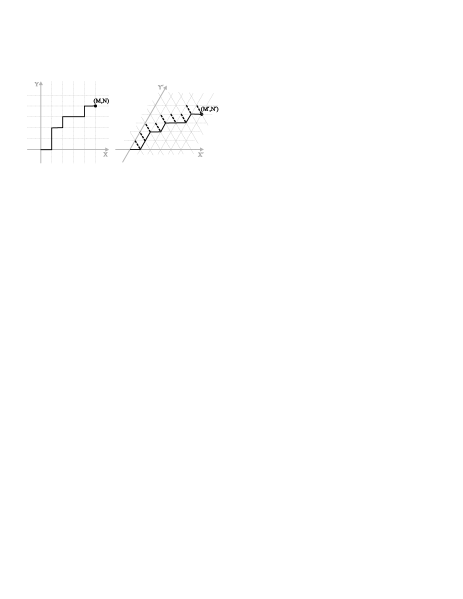
Figure 1: There is a one-to-one correspondence between the shortest-distance steps connecting points on a square lattice [(a), left panel] and the shortest distance steps connecting points on a triangular lattice [(b), right panel]. This figure shows two corresponding steps. Analogous to the $M+N$ broken bonds oriented at $0^{\circ}$ and $90^{\circ}$ on a square lattice, there are $M^{\prime}+N^{\prime}$ broken bonds oriented at $0^{\circ}$ and at $60^{\circ}$ on a triangular lattice. However, there are another $M^{\prime}+N^{\prime}$ broken bonds oriented at $120^{\circ}$ on a triangular lattice.

II.2 Triangular Lattice Step Energy

In order to extend this result to a step on a triangular lattice, we need to make a few minor adjustments. First, we introduce a linear operator $\cal L$ that transforms the coordinates of a point on a square lattice ($M$,$N$) to those on a triangular lattice ($M^{\prime}$,$N^{\prime}$); cf. Fig. 1b. This operator finds the position of a point in a coordinate system whose positive y-axis is bent at $60^{\circ}$ with respect to the positive x-axis:

$$\begin{pmatrix}M^{\prime}\\ N^{\prime}\end{pmatrix} = {\cal L}\begin{pmatrix}M\\ N\end{pmatrix}$$ (5)

$$= \begin{pmatrix}1&-1/\sqrt{3}\\ 0&2/\sqrt{3}\end{pmatrix}\begin{pmatrix}M\\ N\end{pmatrix}.$$

With the aid of $\cal L$, we can see how $E_{0}$ changes on a triangular lattice. To begin, we imagine a step in the first sextant (from $0^{\circ}$ to $60^{\circ}$ degrees in the plane) starting at (0,0) and ending at ($M^{\prime}$, $N^{\prime}$). Such a step is shown in Fig. 1b. As before, the bold solid line represents the step edge with the bottom region a layer higher than the top (or, alternatively phrased, it separates the upper, adatom-free region from the lower, adatom-filled region). The broken bonds required to form the step will have only three orientations: $0^{\circ}$, $60^{\circ}$, and $120^{\circ}$. If we consider the shortest step between the two points (corresponding to energy $E_{0}$), then there will be exactly $M^{\prime}+N^{\prime}$ broken bonds oriented at $0^{\circ}$ and $60^{\circ}$ (these bonds are analogous to those oriented at $0^{\circ}$ and $90^{\circ}$ on a square lattice). There will be another $M^{\prime}+N^{\prime}$ broken bonds oriented at $120^{\circ}$ (drawn as bold, dashed lines in Fig. 1). In total, there will be $2(M^{\prime}+N^{\prime})$ broken bonds. Since $\varepsilon$ is the energy of these severed bonds, $E_{0}^{\vartriangle}=2\varepsilon(M^{\prime}+N^{\prime})$. Thus, the energy is proportional to the step length, as was the case on a square lattice. Using $\cal L$ to write $M^{\prime}$ and $N^{\prime}$ in terms of $M$ and $N$ gives

$$E_{0}^{\vartriangle}=2\varepsilon\left(M+\frac{N}{\sqrt{3}}\right)=2\varepsilon L\left(\cos\theta+\frac{\sin\theta}{\sqrt{3}}\right).$$ (6)

II.3 Triangular Lattice Step Degeneracy

Next we consider the degeneracy factors $g^{\vartriangle}(n)$ on a triangular lattice. For the ground state $g^{\vartriangle}(0)$ there is a one-to-one correspondence between the shortest distance steps connecting two points on a square lattice and the corresponding steps on a triangular lattice (see Fig. 1). Therefore, we know that the degeneracy factor $g^{\vartriangle}_{M^{\prime},N^{\prime}}(0)$ for steps of energy $E_{0}^{\vartriangle}$ on a triangular lattice must be identical to $g_{M^{\prime},N^{\prime}}(0)$ implicit in Eq. (3)! More precisely, if we assume the point ($M$,$N$) is in the first quadrant, and ($M^{\prime}$, $N^{\prime}$) is in the first sextant, then on a square lattice, shortest-distance step-links are oriented at either $0^{\circ}$ or $90^{\circ}$, whereas on a triangular lattice they are oriented at either $0^{\circ}$ or $60^{\circ}$ (i.e. in the first sextant, the shortest path cannot have links oriented at $120^{\circ}$). In both cases, the individual step-links can only be oriented in one of two directions and, therefore, besides the transformation between coordinates, the total number of path arrangements is the same.

Using Eq. (3) and Stirling’s approximation, we find the low-temperature free energy (Appendix I provides the lowest-order correction):

$$F\approx E_{0}^{\vartriangle}-k_{B}T\,\ln[g_{M^{\prime},N^{\prime}}(0)]\approx E_{0}^{\vartriangle}-k_{B}T\times$$ (7)

$$\times\left[(M^{\prime}\!+\!N^{\prime})\ln(M^{\prime}\!+\!N^{\prime})-M^{\prime}\ln M^{\prime}-N^{\prime}\ln N^{\prime}\right].$$

Alternatively, we can transform Eq. (4) for the square lattice to the triangular lattice by just replacing $N/M\equiv\tan\theta$ with $(2\tan\theta)/(\sqrt{3}-\tan\theta)$. (This ratio is just $N^{\prime}/M^{\prime}$, so it might be termed $\tan\theta^{\prime}$.) [We must also make a simple (and ultimately inconsequential) change to $E_{0}$.]

We now take the thermodynamic limit ($M^{\prime}$, $N^{\prime}$ $\gg$ $1$) and write $M^{\prime}$ and $N^{\prime}$ in terms of $M\equiv L\cos\theta$ and $N\equiv L\sin\theta$ via Eq. (5). Then dividing by $L$ and definingA92note

$$\eta_{\pm}(\theta)=\cos\theta\pm\frac{\sin\theta}{\sqrt{3}},\qquad\eta_{0}(\theta)=\frac{2}{\sqrt{3}}\sin\theta,$$ (8)

all non-negative in the first sextant, we straightforwardly find the step-edge line tension (or free-energy per unit lengthIS ) $\beta(\theta)$:

$$a_{\parallel}\beta(\theta)=2\varepsilon\eta_{+}(\theta)-k_{B}T\left[s_{+}(\theta)-s_{-}(\theta)-s_{0}(\theta)\right],$$ (9)

where $a_{\parallel}$ is the nearest-neighbor spacing and

$$s_{i}(\theta)=\eta_{i}(\theta)\ln\eta_{i}(\theta),\quad i=+,0,-\;.$$ (10)

For the special case of the maximally kinked orientation, Eqs. (8) – (10) reduce to

$$a_{k}\beta(30^{\circ})=2\varepsilon-k_{B}T\ln 2,$$ (11)

where $a_{k}=(\sqrt{3}/2)a_{\parallel}$ for the {111} surface. This result for the maximally kinked case (including steps at $\theta\!=\!45^{\circ}$ on a square lattice) was derived earlier from a direct examination of entropy.SGI99

For specificity, we recall some established results. For a hexagonal lattice with just nearest-neighbor attractions, the critical temperature $T_{c}$ is long known:Wan45

$$k_{B}T_{c}=2\varepsilon/\ln 3\approx 1.82\varepsilon\ .$$ (12)

From the equilibrium shape of islands over a broad temperature range, Giesen et al.Ising45 deduced that the free energy per lattice spacing in the maximally kinked directions is 0.27 $\pm$ 0.03eV on Cu{111} and slightly smaller, 0.25 $\pm$ 0.03eV, on Ag{111}. Combining these results with Eq. (11), we find $\varepsilon$ is 0.126eV on Cu{111} and 0.117eV on Ag{111}. In both cases, then, room temperature is somewhere between $T_{c}/9$ and $T_{c}/8$.

II.4 Main Result: Simple Expression for Low-T Stiffness

As shown just above, the step-stiffness $\tilde{\beta}=\beta(\theta)+\beta^{\prime\prime}(\theta)$ computed from Eq. (9) depends to leading order only on the combinatoric entropy terms $s_{0}$ and $s_{\pm}$ of Eqs. (9) and(10). Hence,

$$\frac{d^{2}s_{i}}{d\theta^{2}}\equiv s_{i}^{{}^{\prime\prime}} = -\eta_{i}\ln\eta_{i}+\frac{{\eta_{i}^{{}^{\prime}}}^{2}-\eta_{i}^{2}}{\eta_{i}},$$ (13)

so thatthetanote

$$\tilde{s}_{i} \equiv s_{i}+s_{i}^{{}^{\prime\prime}}=\frac{{\eta_{i}^{{}^{\prime}}}^{2}-\eta_{i}^{2}}{\eta_{i}}.$$ (14)

With this notation, the reduced stiffness is

$$\frac{\tilde{\beta}a_{\parallel}}{k_{B}T} = \tilde{s}_{0}+\tilde{s}_{-}-\tilde{s}_{+},$$ (15)

where

$$\tilde{s}_{0} = \frac{2}{\sqrt{3}}\frac{\cos 2\theta}{\sin\theta},$$ (16)

$$\tilde{s}_{\pm} = \frac{-2\cos 2\theta\mp 2\sqrt{3}\sin 2\theta}{3\cos\theta\pm\sqrt{3}\sin\theta}.$$ (17)

Adding these terms together gives our main result – a remarkably simple form for the reduced stiffness in the low-temperature ($T\ll\varepsilon/k_{B}$) limit:

$$\frac{k_{B}T}{\tilde{\beta}a_{\parallel}}=\frac{\sin(3\theta)}{2\sqrt{3}}=\frac{3m-m^{3}}{2\sqrt{3}(1+m^{2})^{3/2}},$$ (18)

where $m\equiv\tan\theta$.

II.5 Synopsis of Exact Results and Application to Range of Breakdown of Low-T Limit Near $\theta$=0

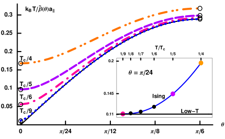
Figure 2: (Color online) As the temperature drops close to $T_{c}/9$ (just below room temperature for Cu and Ag{111} surfaces), the numerical evaluation of the exact stiffnesszia approaches the solid line representing the low-temperature approximation given in Eq. (18). The small circles indicate evaluations using the exact results of Eqs. (23) and (25). At $T_{c}/9$, when $\theta$ decreases, the exact solution begins to deviate from the approximation when its curvature changes sign near $\theta\approx\pi/100=1.8^{\circ}$. The scale here is linear, in contrast to the logarithmic scale of Fig. 2 of Ref. dieluweit02, . The inset shows more fully how the exact stiffness approaches the low-temperature limit for the particular azimuthal angle $\theta\!=\!\pi/24\!=\!7.5^{\circ}$.

To test how low the temperature should be for Eq. (18) to be a good approximation, we compare it to a numerical evaluation of the exact implicit solution of the Ising model. The derivation of this solution, outlined by Zia,zia gives a $6^{th}$ order equation for $\beta(\theta)$. In essence, after conversion to our notation, his key result for the step free energy $\beta$ is given byzianote

$$\frac{\beta a_{\parallel}}{k_{B}T}=\eta_{0}(\theta)\psi_{1}(\theta,T/T_{c})+\eta_{-}(\theta)\psi_{2}(\theta,T/T_{c}),$$ (19)

where the $\psi$’s are the solutions of the pair of simultaneous equations for the angular constraint,

$$\frac{\sinh\psi_{2}-\sinh(\psi_{1}\!-\!\psi_{2})}{\sinh\psi_{1}+\sinh(\psi_{1}\!-\!\psi_{2})}=\frac{\eta_{-}}{\eta_{0}}=\frac{\sqrt{3}\cot\theta-\!1}{2},$$ (20)

and the thermal constraint,

$$\cosh\psi_{1}\!+\!\cosh\psi_{2}\!+\!\cosh(\psi_{1}\!-\!\psi_{2})\!=\!f(z)\!\equiv\!\frac{1+3z^{2}}{2(z-z^{2})},\quad$$ (21)

where $z\equiv\exp(-2\varepsilon/k_{B}T)=3^{-T_{c}/T}$, via Eq. (12). The ratio $\eta_{-}/\eta_{0}$ of Eq. (20) is a monotonically decreasing function which is $\infty$ at $\theta$=0^∘, 1 at $\theta$=30^∘, and 0 at $\theta$=60^∘.

In these high-symmetry directions, Eqs. (20) and (21) yield analytic solutions for $\beta$ and $\tilde{\beta}$:

$$\frac{\beta(0)a_{\parallel}}{k_{B}T} = 2\cosh^{-1}\left(\frac{-1+\sqrt{3+2f}}{2}\right)$$ (22)

$$\frac{\tilde{\beta}(0)a_{\parallel}}{k_{B}T} = \frac{2}{3}\frac{\sqrt{2(3+2f)(f-\sqrt{3+2f})}}{\sqrt{3+2f}-1}$$ (23)

$$\frac{\beta(\raisebox{2.15277pt}{$\pi$}\!/\raisebox{-1.72218pt}{\small 6})a_{\parallel}}{k_{B}T} = \frac{2}{\sqrt{3}}\cosh^{-1}\left(\frac{f-1}{2}\right)$$ (24)

$$\frac{\tilde{\beta}(\raisebox{2.15277pt}{$\pi$}\!/\raisebox{-1.72218pt}{\small 6})a_{\parallel}}{k_{B}T} = \frac{2\sqrt{3(f-3)(f+1)}}{f+3}.$$ (25)

Details are provided in Appendix II. Akutsu and Akutsu AA99 also derived these equations, in different notation AAnote and from the more formal perspective of the imaginary path-weight method. Symmetry dictates that the solution at $\theta=60^{\circ}=\pi/3$ is the same solution as that at $\theta=0^{\circ}$. Furthermore, at $T=T_{c}$, $f(z)=3$, so Eqs. (22)-(25) all go to $0$, as expected.

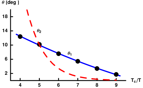
Figure 3: (Color online) Two estimates for the critical angle $\theta_{c}$, below which the approximation given in Eq. (18) begins to fail, as a function of $T_{c}/T$. The black dots connected by the solid, blue line represent the first estimate, defined to be the angle $\theta_{1}$ at which the curvature of the numerically determined inverse stiffness changes sign. The dashed, red line represents the second estimate, $\theta_{2}=\cot^{-1}[(4f-1)/(50\sqrt{3})]$. At angles below $\theta_{c}$, the three theorems of Section III break down, and higher order terms are required in the expansion of the step partition function. At temperatures between $T_{c}/9$ and $T_{c}/8$ (roughly room temperature for Cu and Ag{111} surfaces), $\theta_{c}$ is on the order of a few degrees.

To find $\tilde{\beta}$ in general directions, we solve Eqs. (20) and (21) [or, equivalently, Eq. (39)] numerically. As Fig. 2 shows, once $T$ decreases to nearly $T_{c}/9$, Eq. (18) more or less coincides with the exact numerical solution for the stiffness. At such low temperatures (compared to $T_{c}$), the approximation only fails below some very small, temperature-sensitive critical angle $\theta_{c}$. Although it might seem easy to determine this angle by eye, estimating it quantitatively turns out to be a subtle and somewhat ambiguous task. We discuss two possible estimation techniques below.

In the first approach, we estimate $\theta_{c}$ to be the angle $\theta_{1}$ at which the curvature of the exact solution changes sign. The points on the solid curve in Fig. 3 show $\theta_{1}$ at several temperatures ranging from $T_{c}/9$ to $T_{c}/4$. At temperatures near and above $T_{c}/4$, $\theta_{1}$ does not reliably estimate $\theta_{c}$ because there is a sizable curvature-independent difference between the exact solution and the approximation given in Eq. (18) evident even at $\theta=30^{\circ}$ (see Fig. 2). On the other hand, as the temperature dips below $T_{c}/5$, this difference fades, and the use of $\theta_{1}$ to estimate $\theta_{c}$ becomes ever more precise.

A second, more fundamental way to estimate $\theta_{c}$ comes from an examination of the assumptions required to derive the simple expression for the low-T limit Eq. (18) directly from the exact solutions Eqs. (20) and (21). In Appendix III we show that to do so $\theta$ must be greater than some $\theta_{2}$ satisfying

$$\cot\theta_{2}\ll\left(\frac{4f-1}{\sqrt{3}}\right).$$ (26)

To give definite meaning to this inequality, we estimate $\theta_{c}$ directly from Fig. 2 at a single temperature, say $T_{c}/5$. At that temperature, $\theta_{c}$ is nearly $10^{\circ}$. If $\theta_{2}$ is to accurately represent $\theta_{c}$, it should also be around $10^{\circ}$ at $T_{c}/5$. We enforce this by interpreting the ‘$\ll$’ in Eq. (26) to mean ‘$=1/50$.’ The dashed (red online) curve in Fig. 3 shows the resulting $\theta_{2}$ as a function of temperature.

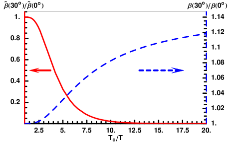
Figure 4: (Color online) Ratio of the stiffness [solid red curve, left ordinate] and the free energy per length [dashed blue curve, right axis] for edges oriented in the maximally zig-zagged ($\theta=30^{\circ}$) and close-packed ($\theta=0^{\circ}$) directions, based on taking the ratios of Eqs. (25) and (23) and of Eqs. (24) and (22), respectively. The line-tension ratio increases slowly but monotonically to the $T$=0 limit $2/\sqrt{3}\approx 1.15$. In contrast, the stiffness ratio plummets toward 0, the value predicted by Eq.(18), providing an indicator how low $T$ must be for this simple low-$T$ formula to be a good approximation at all angles.

Clearly $\theta_{1}$ and $\theta_{2}$ are very different estimates for $\theta_{c}$. While $\theta_{2}$ is reliable at all temperatures (unlike $\theta_{1}$), it is less precise than $\theta_{1}$ at lower temperatures. A combination of $\theta_{1}$ and $\theta_{2}$ is therefore the best estimate for $\theta_{c}$, being closer to $\theta_{1}$ at lower temperatures, and closer to $\theta_{2}$ at higher temperatures.

In essence, $\theta_{c}$ is no more than a few degrees between $T_{c}/9$ and $T_{c}/8$, regardless of which estimation technique is used. We therefore reach the practical conclusion that Eq. (18) is valid for almost all angles at temperatures near and below $T_{c}/8$, which fortunately happens to be around room temperature for Cu and Ag{111}.

Finally, we emphasize that $\tilde{\beta}$ varies significantly with angle, especially at lower temperatures (where the equilibrium crystal shape (ECS) is hexagonal rather than circular). If one wants to approximate $\tilde{\beta}$ as isotropic rather than using Eq. (18), one should not pick its value in the close-packed direction (viz. $\theta=0^{\circ}$); Fig. 4 provides stunning evidence of this conclusion. From Eq. (18) we also see that at low-temperatures the stiffness actually increases linearly with temperature. This contrasts with its behavior at high temperatures, where $\tilde{\beta}$ must ultimately decrease as the ECS becomes more nearly circular and the steps fluctuate more easily.

III General Results for Stiffness in Lattice-gas Models in Low-Temperature Approximation

In this section we present three theorems that are valid under two conditions: First, the energy term in the free energy must be a linear combination of $\cos\theta$ and $\sin\theta$. From Eq. (6) and [implicitly] Eq. (3) we see that this property holds true in general for lattice-gas models, even when considering next-nearest neighbors and beyond.Herring51 Second, the temperature must be low enough so that the entropy is adequately approximated by the contribution of the lowest order term, $k_{B}\ln g(0)$. This entropic contribution is due exclusively to geometry or combinatorics of arranging the fixed number of kinks forced by azimuthal misorientation. Hence, it must vanish near close-packed directions (0^∘ and 60^∘ in the first sextant). For angles sufficiently close to these directions, in our case less than $\theta_{c}$, the leading term becomes dominated by higher-order terms, and the three results no longer apply.

III.1 No Contribution from Energy to Lowest-Order Stiffness (LOS)

The first theorem is a remarkable consequence of the first condition, that the energy term in the free energy is a linear combination of $\cos\theta$ and $\sin\theta$. Since the stiffness $\tilde{\beta}(\theta)\equiv\beta(\theta)+\beta^{\prime\prime}(\theta)$ and since $\cos^{\prime\prime}\theta=-\cos\theta$ and $\sin^{\prime\prime}\theta=-\sin\theta$, we see that the lattice-gas energy makes no contribution whatsoever to the low-T limit of reduced stiffness, as shown explicitly for square lattices long ago.rottman ; Cahn Thus, we retrieve the result that the leading term in a low-temperature expansion of the reduced stiffness $\tilde{\beta}(\theta)/k_{B}T$ depends only on $g(0)$, which is determined solely by geometric (combinatoric) properties. Of course, higher-order terms (which are crucial near close-packed directions) do have weightings of the various configurations that depend on Boltzmann factors involving the characteristic lattice-gas energies. Furthermore, next-nearest-neighbor interactions can (at least partially) lift the $g(0)$-fold degeneracy of the lowest energy paths.tjs001

III.2 Step Line Tension Not Extractable from LOS

An important corollary is that from the stiffness it is impossible to retrieve the energetic part of the step free energy, the major component of $\beta(\theta)$ at lower temperatures when the islands are non-circular! Thus, contrary to a proposed method of data analysis,OSDF one cannot regenerate $\beta(\theta)$ from $\tilde{\beta}(\theta)$ by fitting the stiffness to a simple functional form and then integrating twice. In this framework, the linear coefficients of $\cos\theta$ and $\sin\theta$ can be viewed as the two integration constants associated with integrating a second-order differential equation.Krug03

III.3 LOS on fcc{111} Has 6-fold Symmetry

III.3.1 1. General Argument

Another important result is that the leading term in the stiffness at low temperature has the full symmetry of the 2D net of binding sites rather than the possibly lower symmetry associated with the full lattice. Specifically, for the present problem of the {111} face of an fcc crystal, the stiffness $\tilde{\beta}(\theta)$ to lowest order has the full 6-fold symmetry of the top layer rather than the 3-fold symmetry due to symmetry breaking by the second layer. In contrast, the step energy of B-steps ({111} microfacets) differs from that of A-steps ({100} microfacets), leading to islands with the shape of equiangular hexagons with rounded corners, but with sides of alternating lengths (i.e., ABABAB).

To see the origin of the 6-fold symmetry of the stiffness, suppose without loss of generality that steps in the $X^{\prime}$ direction have energy $E_{A}$ per lattice spacing, so that those in the $Y^{\prime}$ direction have energy $E_{B}$. Furthermore, we must make the crucial assumption that any corner energy is negligible. Then all shortest paths to ($M^{\prime},N^{\prime}$) have the same energy $M^{\prime}E_{A}+N^{\prime}E_{B}$, with degeneracy still $g_{M^{\prime},N^{\prime}}(0)$. Thus, the free energy is $M^{\prime}E_{A}+N^{\prime}E_{B}-k_{B}T\ln g_{M^{\prime},N^{\prime}}(0)$, while that of its mirror point (through the line at $\theta=30^{\circ}$) is $N^{\prime}E_{A}+M^{\prime}E_{B}-k_{B}T\ln g_{N^{\prime},M^{\prime}}(0)$. The crux of the proof is that $g_{N^{\prime},M^{\prime}}(0)=g_{M^{\prime},N^{\prime}}(0)$. Thus, while the free energies at the pair of mirror points differ, the energy parts are obliterated when the stiffness is computed (since $M^{\prime}$ and $N^{\prime}$ are linear combinations of $\cos\theta$ and $\sin\theta$), leaving just the contribution from the entropies, which are the same to lowest order.

III.3.2 2. Orientation-Dependent 3-Atom Interaction

Within lattice-gas models with only pair interactions, there is no obvious way to distinguish A and B steps; the minimalist way to obtain different step energies for A and B steps within the lattice-gas model is to invoke a non-pairwise 3-site “trio” interaction associated with three [occupied] sites forming an equilateral triangle with NN sides. In contrast to the ones considered heretofore,triorev ; TLE-Unertl these novel trio interactions must be orientation-dependent: If the triangle points in one direction, say up, the interaction energy is positive, while if it points in the opposite direction, it has the opposite sign. (Of course, there could be a standard orientation-independent 3-site term in the Hamiltonian. As in the analogous situation for squares, we expect that such a term would simply shift the pair interactions, at least in the SOS approximation as discussed in Ref. tjs001, .) The contributions from such a symmetry-breaking interaction would cancel in the interior of an island (in the 2D bulk), but would distinguish A and B edges. Specifically, each side of the equilateral triangle is associated with a link, so that 1/3 of its strength can be attributed to each. Each link has a triangle on both sides, one of each orientation. Hence, the difference between the energy per $a_{\parallel}$ of A and B steps is 1/3 the difference between the trio interactions in the two opposite orientations.

For the ground-state, minimum-number-of-links configurations, such a term will not lift the degeneracy since each configuration has the same 1) number of horizontal ($X^{\prime}$) links, 2) number of right-tilted diagonal links ($Y^{\prime}$), and 3) difference between the number of convex and concave “kinks” (i.e., bends). Since this statement is not true for higher-energy configurations, the 6-fold symmetry is not preserved at higher orders. Nonetheless, at low $T$ it should be a decent approximation for the stiffness (much better than for the island shape).

Thus, our result that the breaking of 6-fold symmetry on an fcc {111} is much smaller for the stiffness than for the free energy, is more general than the nearest-neighbor lattice gas model which underlies Eqs. (9) – (10) and the resulting Eq. (18) derived below. We reemphasize that the necessary assumptions are 1) that the orientational dependence of the step energy be just a linear combination of $\sin\theta$ and $\cos\theta$ and 2) that no interaction break the degeneracy of the shortest path corresponding to orientation $\theta$. As above, for angles near close-packed directions, the higher-order terms become important at lower temperatures than for general directions. This feature is illustrated in Fig. 2 and its associated formalism is given in Appendices I and III.

IV Comparison to Experiment

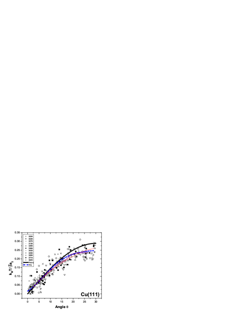
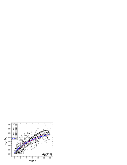
Figure 5: (Color online) A comparison between Eq. (18) and experiments on Cu and Ag{111}. Eq. (18) appears as a solid black line, while the average of the experimental data is a thick dashed blue line. The agreement is reasonable at all angles. In either case the thin dashed red line is a [smoothed] average of the data for the given angle while the thin solid purple line corresponds to the angle mirror-reflected through a radial at 30^∘, i.e. at 60${}^{\circ}\!-\!\theta$.

In Fig. 5 we compare Eq. (18) to measurements on Cu{111} and Ag{111}. The experimental data were derived from the equilibrium shape of 2D islands using the method described in Ref. dieluweit02, . The solid black line corresponds to Eq. (18), while the thick dashed blue line corresponds to the average of the experimental measurements. Eq. (18) captures the overall trend and is satisfactory at most angles and temperatures. As expected, Eq. (18) somewhat overestimates $\tilde{\beta}$ near $\theta=0^{\circ}$ (since the $T\!=\!0$ singularity remains). Furthermore, near $\theta=30^{\circ}$ Eq. (18) somewhat underestimates the experimental $\tilde{\beta}$, but only by a factor of 1/6 for Cu{111} and 1/4 for Ag{111}. This is in striking contrast to the analogous NN theory for Cu{001} near 45^∘, which underestimates $\tilde{\beta}$ by a factor of 4. Finally, notice there is no clear temperature dependence in the measured data. This is further evidence that $\tilde{\beta}/k_{B}T$ is a constant at low-temperatures, as Eq. (18) suggests.

The agreement between theory and experiment is a pleasant surprise considering analogous comparisons made for Cu{001}dieluweit02 found $\tilde{\beta}$ to be four-times larger than the theoretical value at large angles (near $\theta=45^{\circ}$). It was later shownZP1 ; ZP2 ; tjs001 that this discrepancy could be partially accounted for by considering next-nearest-neighbor (NNN) interactions (or right-triangle trio interactions, which turn out to affect $\tilde{\beta}$ at low temperatures in the same way). Clearly, the success of Eq. (18) suggests that these interactions are less relevant for {111} surfaces. This is reasonable because the ratio of NNN distance to NN distance is smaller by a factor of $\sqrt{2/3}$ on a triangular lattice compared to on a square lattice. Furthermore, in the close-packed direction ($\theta=0^{\circ}$), for every broken NN-bond there are only one and a half broken NNN bonds on a triangular lattice, compared to two broken NNN bonds on a square lattice. These simple arguments help explain why NNN-interactions may increase $\tilde{\beta}$ by only $20$ to $30$% on Cu/Ag{111}, as opposed to $400$% on Cu{001} surfaces.

V Concluding Discussion

By generalizing the low-temperature expansion of the nearest-neighbor square lattice-gas (Ising) model to a triangular lattice, we have found a remarkably simple formula for the orientation dependence of the {111} surface step stiffness. This formula, unlike its square lattice analog, fits experimental data well at general angles, suggesting that NNN-interactions are relatively unimportant on {111} surfaces.

To corroborate this picture and explain the success of Eq. (18), we are currently using the VASP packageVASP to perform first-principle calculations. In particular, we are examining the ratio of the NNN to NN interaction strength. Preliminary resultsSTK suggest that this ratio is roughly an order of magnitude smaller on Cu{111} than on Cu{001}, and essentially indistinguishable from zero. This tentative finding is consistent with expectations from the semiempirical embedded atom method, which predicts that indirect interactions are insignificant/negligible between atoms sharing no common substrate atoms.TLE-Unertl We are also calculating the difference in trio interactions between oppositely oriented triangle configurations.

We expect that our formula, as well as the general 6-fold symmetry of the stiffness (except in close-packed directions), should be broadly applicable to systems in which multisite or corner energies are small and for which the bond energies are considerably higher than the measurement temperature. Studies which ignore the 3-fold symmetry breaking on metallic fcc {111} substrates, such as a recent investigation of nanoisland fluctuations on Pt{111},Sz04 should be good representations. Many recent investigationsDanker ; KK04 focus on the larger asymmetry of the kinetic coefficient,GD04 taking the stiffness to be isotropic. In such cases, this stiffness should not be characterized by its value in close-packed directions.

APPENDIX I: LEADING TERM IN LOW-TEMPERATURE EXPANSION

V.1 Review of Results for Square Lattice

In this appendix we discuss the lowest-order correction to the ground state entropy of the step running from the origin to an arbitrary particular point. First we review results for a square lattice. We can rewrite Eq. (2) as

$$Z_{\theta}=g_{M,N}(0)e^{-E_{0}/kT}\left[1+\frac{g_{M,N}(1)}{g_{M,N}(0)}e^{-\Delta E/kT}+...\right].$$ (27)

Then, assuming the exponential is small, we have

$$F\approx E_{0}-k_{B}T\left\{\ln[g_{M,N}(0)]+\frac{g_{M,N}(1)}{g_{M,N}(0)}e^{-2\varepsilon/k_{B}T}\right\}.$$ (28)

A combinatorial analysisCahn ; rottman ; tjsnote1 shows that

$$g_{M,N}(1)={M\!+\!N\choose M\!-\!1}(M\!+\!1)+{M\!+\!N\choose N\!-\!1}(N\!+\!1)$$ (29)

Then Eq. (4) generalizes to

$$F \approx E_{0}-k_{B}T\left[(M\!+\!N)\ln(M\!+\!N)-M\ln M-N\ln N\right.$$ (30)

$$\left.+e^{-2\varepsilon/k_{B}T}\frac{M^{3}+N^{3}}{MN}\right].$$

V.2 Results for Triangular Lattice

For the triangular lattice we find important differences from the square lattice for the higher-order terms. Specifically, we consider how $g(1)$ changes. In contrast to $g(0)$, we cannot simply replace $M$ and $N$ with $M^{\prime}$ and $N^{\prime}$. There is no one-to-one correspondence between paths of energy $E_{1}$ on a square lattice and those of energy $E_{1}^{\vartriangle}$ on a triangular lattice. This failed correspondence for higher terms follows from the observation that $E_{1}^{\vartriangle}$-configurations are only one link longer than $E_{0}^{\vartriangle}$-steps, whereas $E_{1}$-configurations are two links longer than $E_{0}$-steps: $E_{n+1}^{\vartriangle}-E_{n}^{\vartriangle}\equiv\Delta E^{\vartriangle}=\varepsilon$, or

$$E_{n}^{\vartriangle}=\varepsilon\left(\frac{2N}{\sqrt{3}}+2M+n\right),\,n=0,1,2,...,$$ (31)

Hence, we require a separate combinatorial analysis.

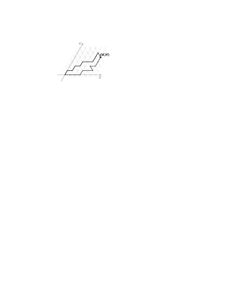
Figure 6: Two equivalent steps having energy $E_{1}^{\vartriangle}$. The dashed step contains ($M^{\prime}+1$) X-links, ($N^{\prime}-1$) Y-links, and one $\Upsilon$-link, while the solid step contains ($M^{\prime}-1$) X-links, ($N^{\prime}+1$) Y-links, and one $\Upsilon$-link.

We imagine a step of energy $E_{1}$ in the first sextant. Such a step (see Fig. 6) will have either: (1) ($M^{\prime}+1$) links oriented at $0^{\circ}$ (denoted “X-links”), ($N^{\prime}-1$) links oriented at $60^{\circ}$ (denoted “Y-links”), and one link oriented at $120^{\circ}$ (denoted “$\Upsilon$-links”), or (2) ($M^{\prime}-1$) links oriented at $0^{\circ}$, ($N^{\prime}+1$) links oriented at $60^{\circ}$, and one link oriented at $-60^{\circ}$. In the first case, the problem can be reworded as follows: how many ways to arrange an ($M^{\prime}+N^{\prime}+1$)-lettered word with ($M^{\prime}+1$) X’s, ($N^{\prime}-1$) Y’s, and one $\Upsilon$. In the second case, the problem is the same, only with $M$ and $N$ switched. Thus, the solution of this traditional combinatorial problem gives the total number of next-to-shortest paths $g^{\vartriangle}(1)$:

$$g^{\vartriangle}(1)={M^{\prime}\!+\!N^{\prime}\!+\!1\choose M^{\prime}\!+\!1}N^{\prime}+{M^{\prime}\!+\!N^{\prime}\!+\!1\choose N^{\prime}\!+\!1}M^{\prime}.$$ (32)

With $g^{\vartriangle}(0/1)$ and $E_{n}^{\vartriangle}$ in hand, we can write the low-temperature partition function expansion for a triangular lattice. Using Eq. (3) and expanding the logarithm as in Eq. (28), we have

$$F \approx E_{0}^{\vartriangle}-k_{B}T\,\left\{\ln[g(0)]+\frac{g^{\vartriangle}(1)}{g(0)}e^{-\Delta E^{\vartriangle}/k_{B}T}\right\}.$$ (33)

Taking the thermodynamic limit ($M^{\prime}$, $N^{\prime}$ $\gg$ $1$) and using Stirling’s approximation gives

$$F\! \approx \!E_{0}^{\vartriangle}\!-\!k_{B}T\left[(M^{\prime}\!+\!N^{\prime})\ln(M^{\prime}\!+\!N^{\prime})\!-\!M^{\prime}\ln M^{\prime}\!-\!N^{\prime}\ln N^{\prime}\right.$$ (34)

$$+ \!\left.e^{-\varepsilon/k_{B}T}\frac{M^{\prime 3}\!+\!N^{\prime 3}\!+\!M^{\prime}N^{\prime 2}\!+\!N^{\prime}M^{\prime 2}}{M^{\prime}N^{\prime}}\right]\,.$$

The pair of cross-factors in the last coefficient are absent in Eq. (30) for the square lattice.

The correction term becomes non-negligible when the final term in Eq. (34) becomes of order unity. At low $T$ this occurs only near close-packed directions, so for small values of $\theta$. In this regime, to lowest order in $\theta$, $N^{\prime}=(2L/\sqrt{3})\sin\theta\rightarrow 2L\theta/\sqrt{3}$ and $M^{\prime}=L\cos\theta-N^{\prime}/2\rightarrow L$. Then the critical value of $\theta$ is

$$\theta_{c}^{(\beta)}\approx\textstyle{\frac{\sqrt{3}}{2}}e^{-\varepsilon/k_{B}T}=\textstyle{\frac{\sqrt{3}}{2}}z^{1/2}.$$ (35)

Specifically, based on Eq. (35) and using $\varepsilon\approx 0.12$ eV for Cu{111}, we find that $\theta_{c}^{(\beta)}$ is 0.353^∘, 3.18^∘, and 5.51^∘ for T/T_c of 1/9, 1/5, and 1/4, respectively. As clear from Fig. 3, this criterion turns out to underestimate the values for $\theta_{c}$ obtained in Section II.D, mainly because Eq. (35) was derived from an expression for $\beta(\theta)$ instead of $\tilde{\beta}(\theta)$ (which should depend more sensitively on $\theta$). over the plotted thermal range.

APPENDIX II: EXACT FORMULAS FOR LINE TENSION AND STIFFNESS IN MIRROR DIRECTIONS

A. General results for all orientations

In this appendix, we derive Eqs. (22) – (25) for the mirror-line directions $\theta=0^{\circ}$ and $\theta=30^{\circ}$ from Zia’s implicit exact solution.zia

To begin, because $\tilde{\beta}=\beta+\beta^{\prime\prime}$ (where the prime represents differentiation with respect to $\theta$), it follows from Eq. (19) that

$$\frac{\tilde{\beta}a_{||}}{k_{B}T}=2\eta_{0}^{\prime}\psi_{1}^{\prime}+2\eta_{-}^{\prime}\psi_{2}^{\prime}+\eta_{0}\psi_{1}^{\prime\prime}+\eta_{-}\psi_{2}^{\prime\prime}.$$ (36)

We can simplify Eq. (36) by finding relationships between the various derivatives of the $\psi$’s. Differentiating Eq. (21) with respect to $\theta$, regrouping, and using Eq. (20), we get

$$\psi_{1}^{\prime}\eta_{0}+\psi_{2}^{\prime}\eta_{-} = 0.$$ (37)

Differentiating again yields

$$\psi_{1}^{\prime\prime}\eta_{0}+\psi_{2}^{\prime\prime}\eta_{-}+\psi_{1}^{\prime}\eta_{0}^{\prime}+\psi_{2}^{\prime}\eta_{-}^{\prime} = 0.$$ (38)

Using Eq. (38), we rewrite the last part of Eq. (36) (containing $\psi_{1}^{\prime\prime}$ and $\psi_{2}^{\prime\prime}$) in terms of just $\psi_{1}^{\prime}$ and $\psi_{2}^{\prime}$. Then, using Eq. (37) we eliminate $\psi_{2}^{\prime}$ in favor of $\psi_{1}^{\prime}$. We are then left with an equation relating $\tilde{\beta}$ to only $\psi_{1}^{\prime}$:

$$\frac{\tilde{\beta}a_{||}}{k_{B}T}=\left(\eta_{0}^{\prime}-\eta_{-}^{\prime}\frac{\eta_{0}}{\eta_{-}}\right)\psi_{1}^{\prime}=\frac{2\psi_{1}^{\prime}}{\sqrt{3}\cos\theta-\sin\theta}.$$ (39)

For general angle, we must evaluate $\psi_{1}^{\prime}$ numerically. However, for the two high-symmetry directions we can obtain analytic results that allow us (with the aid of Eq. (19) for $\beta$) to write explicit expressions for $\tilde{\beta}$, as presented in the next two subsections.

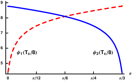
Figure 7: (Color online) Numerical evaluation of $\psi_{1}$ (dashed red curve) and $\psi_{2}$ (solid blue curve) as functions of angles at temperature $T_{c}/8$ equivalent to room temperature for the experimental systems Cu and Ag {111}. Note that the linear behavior near one limit and the divergent slope near value zero at the other. At higher temperatures the curves are qualitatively similar but progressively smaller in magnitude.

B. Results for $\theta=0^{\circ}$

At $\theta=0^{\circ}$, Eq. (19) reduces to

$$\frac{\beta a_{||}}{k_{B}T}=\psi_{2}(0),$$ (40)

assuming that $\psi_{1}(0)$ is finite. Furthermore, near $\theta=0^{\circ}$, Eq. (20) can be inverted and the $\sinh$’s combined to get

$$\frac{\sinh(\psi_{1}-\frac{1}{2}\psi_{2})\cosh(\frac{1}{2}\psi_{2})}{\sinh(\psi_{2}-\frac{1}{2}\psi_{1})\cosh(\frac{1}{2}\psi_{1})}=\frac{2}{\sqrt{3}}~{}\theta.$$ (41)

For Eq. (41) to hold at $\theta=0^{\circ}$,

$$\psi_{2}(0)=2\psi_{1}(0).$$ (42)

Eq. (21) therefore becomes:

$$2\cosh\psi_{1}(0)+\cosh(2\psi_{1}(0))=f.$$ (43)

Solving this for $\cosh\psi_{1}(0)$ and taking the positive root, we find:

$$\cosh\psi_{1}(0)=\cosh(\textstyle{\frac{1}{2}}\psi_{2}(0))=\textstyle{\frac{1}{2}}(-1+\sqrt{3+2f}),$$ (44)

consistent with the assumption of finite $\psi_{1}(0)$. Solving for $\psi_{2}(0)$ and combining with Eq. (40) yields Eq. (22).

Correspondingly for $\tilde{\beta}$, at $\theta=0^{\circ}$ Eq. (39) becomes

$$\frac{\tilde{\beta}(0)a_{\parallel}}{k_{B}T} = \frac{2}{\sqrt{3}}\psi_{1}^{\prime}(0),$$ (45)

while Eq. (37) becomes

$$\psi_{2}^{\prime}(0)=0,$$ (46)

provided $\psi_{1}^{\prime}(0)$ is finite. We obtain $\psi_{1}^{\prime}(0)$ by differentiating Eq. (41) with respect to $\theta$ and then setting $\theta=0^{\circ}$ so that Eqs. (42) and (46) apply. This give

$$\psi_{1}^{\prime}(0)=\textstyle{\frac{1}{\sqrt{3}}}\tanh\psi_{1}(0)[1+2\cosh\psi_{1}(0)].$$ (47)

By combining this with Eq. (44) for $\cosh\psi_{1}(0)$, we see that $\psi_{1}^{\prime}(0)$ is indeed finite, as we earlier assumed. Thus, Eq. (45) becomes Eq. (23), as desired.

C. Results for $\theta=30^{\circ}$

At $\theta=30^{\circ}=\pi/6$, Eq. (19) becomes

$$\frac{\beta(\raisebox{1.72218pt}{$\pi$}\!/\raisebox{-1.29167pt}{\footnotesize 6})a_{\parallel}}{k_{B}T} = \textstyle{\frac{1}{\sqrt{3}}}\left[\psi_{1}(\raisebox{2.15277pt}{$\pi$}\!/\raisebox{-1.72218pt}{\small 6})+\psi_{2}^{\prime}(\raisebox{2.15277pt}{$\pi$}\!/\raisebox{-1.72218pt}{\small 6})\right].$$ (48)

Furthermore, near $\theta=\pi/6$, $\eta_{0}/\eta_{-}\approx 1+2\sqrt{3}~{}\Delta\theta$, where $\Delta\theta\equiv\theta-\pi/6$. Inverting Eq. (20) we therefore have

$$\frac{\sinh\psi_{1}+\sinh(\psi_{1}-\psi_{2})}{\sinh\psi_{2}-\sinh(\psi_{1}-\psi_{2})}\approx 1+2\sqrt{3}~{}\Delta\theta,$$ (49)

By inspection, at $\theta=\pi/6$ ($\Delta\theta=0$), one solution to this equation is just

$$\psi_{2}(\raisebox{2.15277pt}{$\pi$}\!/\raisebox{-1.72218pt}{\small 6})=\psi_{1}(\raisebox{2.15277pt}{$\pi$}\!/\raisebox{-1.72218pt}{\small 6}).$$ (50)

Plugging this result into Eq. (21) and solving for $\psi_{2}(\pi/6)$ gives,

$$\cosh\psi_{2}(\raisebox{2.15277pt}{$\pi$}\!/\raisebox{-1.72218pt}{\small 6})=\frac{f-1}{2}.$$ (51)

Combining this with Eq. (48) (where we now know $\psi_{1}(\pi/6)=\psi_{2}(\pi/6)$) results in Eq. (24).

As for $\tilde{\beta}$, at $\theta=\pi/6$, Eq. (39) becomes

$$\frac{\tilde{\beta}a_{||}}{k_{B}T}=2\psi_{1}^{\prime}(\raisebox{2.15277pt}{$\pi$}\!/\raisebox{-1.72218pt}{\small 6}),$$ (52)

while Eq. (37) becomes

$$\psi_{1}^{\prime}(\raisebox{2.15277pt}{$\pi$}\!/\raisebox{-1.72218pt}{\small 6})=-\psi_{2}^{\prime}(\raisebox{2.15277pt}{$\pi$}\!/\raisebox{-1.72218pt}{\small 6}).$$ (53)

Like before, we can find $\psi_{1}^{\prime}(\pi/6)$ by differentiating Eq. (49) with respect to $\theta$. Taking the result and setting $\theta=\pi/6$, so that Eqs. (50) and (53) apply, gives

$$\psi_{1}^{\prime}(\raisebox{2.15277pt}{$\pi$}\!/\raisebox{-1.72218pt}{\small 6})=\frac{\sqrt{3}\sinh\psi_{1}}{\cosh\psi_{1}+2}.$$ (54)

Finally, we combine this result with Eq. (51) for $\cosh\psi_{2}(\raisebox{2.15277pt}{$\pi$}\!/\raisebox{-1.72218pt}{\small 6})=\cosh\psi_{1}(\raisebox{2.15277pt}{$\pi$}\!/\raisebox{-1.72218pt}{\small 6})$ and Eq. (52), to get Eq. (25), as desired.

APPENDIX III: REDERIVATION OF EQ. (18) FROM EXACT SOLUTION

In this appendix, we re-derive Eq. (18) directly from the exact solution for $\beta(\theta)$ given in Eqs. (20) and (21). To do so, we just assume $\cosh\psi_{2}\gg\eta_{-}/\eta_{0}$ (remember that $\eta_{-}/\eta_{0}$ decreases from $\infty$ at $\theta=0^{\circ}$ to 1 at $\theta=30^{\circ}$, so that, between these angles, this condition also implies that $\cosh\psi_{2}\gg 1$). In this case, Eq. (20) can be solved to give

$$\cosh\psi_{1}\approx\frac{\eta_{0}}{\eta_{-}}\cosh\psi_{2}.$$ (55)

Thus, if $\cosh\psi_{2}\gg\eta_{-}/\eta_{0}>1$, then $\cosh\psi_{1}\gg 1$. We show here that these assumptions for $\cosh\psi_{1,2}$, together with the low-temperature replacement of $f(z)$ by $1/(2z)$ in Eq. (21), are enough to derive Eq. (18).

When $\cosh\psi_{1,2}\gg 1$, then $\cosh\psi_{1,2}\approx\sinh\psi_{1,2}\approx e^{\psi_{1,2}}/2$. With these approximations, Eqs. (20) and (21) become remarkably simple:

$$e^{\psi_{1}}+e^{\psi_{2}} = 2f(z),$$ (56)

$$e^{\psi_{2}} = \frac{\eta_{-}}{\eta_{0}}e^{\psi_{1}}.$$ (57)

Solving this pair of equations for $e^{\psi_{1}}$ and $e^{\psi_{2}}$ gives

$$e^{\psi_{1}}=\frac{2f(z)\eta_{0}}{\eta_{0}+\eta_{-}},\qquad e^{\psi_{2}}=\frac{2f(z)\eta_{-}}{\eta_{0}+\eta_{-}}.$$ (58)

If we then replace $f(z)$ by its low-temperature limit, $1/(2z)$, Eq. (19) becomes

$$\frac{\beta a_{||}}{k_{B}T}=\eta_{0}\ln\left[\frac{\eta_{0}}{z(\eta_{0}+\eta_{-})}\right]+\eta_{-}\ln\left[\frac{\eta_{-}}{z(\eta_{0}+\eta_{-})}\right].$$ (59)

By noting $\eta_{0}+\eta_{-}=\eta_{+}$, and using the definition for $z$, Eq. (59) can be easily simplified to Eq. (9), from which Eq. (18) for $\tilde{\beta}$ was derived.

By deriving the approximation given in Eq. (9) (and thus Eq. (18)) in this way, we can determine when the approximation becomes invalid. Specifically, we require $\cosh\psi_{1,2}\gg 1$. As we showed, the more restrictive of these inequalities is the one involving $\cosh\psi_{1}$, since $\cosh\psi_{1}$ is necessarily smaller than $\cosh\psi_{2}$ in the first sextant by a factor of $\eta_{0}/\eta_{-}$ (which is less than 1). Thus, the main assumption is $\cosh\psi_{1}\gg 1$, which, from Eq. (58), is just

$$\frac{2f(z)\eta_{0}}{\eta_{0}+\eta_{-}}\gg 1.$$ (60)

The solution to this equation, which we call $\theta_{2}$, is given by the following inequality:

$$\cot\theta_{2}\ll\frac{4f-1}{\sqrt{3}}.$$ (61)

Because $\cot\theta$ decreases from $\infty$ at $\theta=0$ to $1/\sqrt{3}$ at $\theta=\pi/6$, we know that angles in the first sextant that are greater than $\theta_{2}$ will also satisfy the inequality in Eq. (61). Thus, Eqs. (9) and (18) are valid in the first sextant at all angles above $\theta_{2}$.

- (1) H.-C. Jeong and E. D. Williams, Surf. Sci. Rept. 34, 171 (1999).
- (2) D. B. Abraham and P. Reed, J. Phys. A 10, L8121 (1977).
- (3) C. Rottman and M. Wortis, Phys. Rev. B 24, 6274 (1981).
- (4) J.E. Avron, H. van Beijeren, L. S. Schulman, and R. K. P. Zia, J. Phys. A 15, L81 (1982); R. K. P. Zia and J.E. Avron, Phys. Rev. B 25, 2042 (1982).
- (5) R. K. P. Zia, J. Stat. Phys. 45, 801 (1986).
- (6) S. Dieluweit, H. Ibach, M. Giesen, and T. L. Einstein, Phys. Rev. B 67, 121410 (2003).
- (7) R. Van Moere, H. J. W. Zandvliet, and B. Poelsema, Phys. Rev. B 67, 193407 (2003).
- (8) H. J. W. Zandvliet, R. Van Moere, and B. Poelsema, Phys. Rev. B 68, 073404 (2003).
- (9) T. J. Stasevich, T. L. Einstein, R. K. P. Zia, M. Giesen, H. Ibach, and F. Szalma, Phys. Rev. B 70, xxx (15 Nov. 2004) [cond-mat/0408496].
- (10) M. Giesen, C. Steimer, and H. Ibach, Surf. Sci. 471, 80 (2001).
- (11) J. W. Cahn and R. Kikuchi, J. Phys. Chem. Solids 20, 94 (1961).
- (12) In deriving the equivalent of our Eq. (9) for honeycomb lattices, N. Akutsu, J. Phys. Soc. Jpn. 61, 477 (1992) noted that what we call can be written .
- (13) This simple equivalency does not hold for stepped surfaces in an electrochemical system, where the electrode potential is fixed rather than the surface charge density conjugate to . H. Ibach and W. Schmickler, Phys. Rev. Lett. 91, 016106 (2003). Other noteworthy subtleties in the free energy are discussed by N. Akutsu and Y. Akutsu, J. Phys. Soc. Jpn. 64, 736 (1995).
- (14) G. Schulze Icking-Konert, M. Giesen, and H. Ibach, Phys. Rev. Lett. 83, 3880 (1999).
- (15) G. H. Wannier, Rev. Mod. Phys. 17, 50 (1945).
- (16) The calculation can be facilitated by writing and then using Eq. (14) to show .
- (17) Eq. (21) bypasses several intermediate quantities that are important for Zia’s [zia, ] general treatment but cumbersome here. Our has the opposite sign from Zia’s, and our angle —which vanishes for close-packed step orientations—differs by 30∘ from his. Note also that interchanging and on the LHS of Eq. (20) inverts the LHS, from which it is easy to see that of Eq. (19) is symmetric about . The LHS of Eq. (21) is obviously invariant under the interchange of and .
- (18) N. Akutsu and Y. Akutsu, J. Phys.: Condens. Matter 11, 6635 (1999).
- (19) In Eqs. (4.30)-(4.33) of Ref. AA99, , their corresponds to our and their angles, like Zia’s [zia, ; zianote, ], differ from ours so that their is our 0 and their 0 is our .
- (20) C. Herring, Phys. Rev. 82, 87 (1951).
- (21) M. Ondrejcek, W. Swiech, C. S. Durfee, and C. P. Flynn, Surf. Sci. 541, 31 (2003).
- (22) J. Krug, private communication.
- (23) T. L. Einstein, Langmuir 7, 2520 (1991); G. Ehrlich and F. Watanabe, ibid. 2555; B.N.J. Persson, Surf. Sci. Repts. 15, 1 (1992).
- (24) T. L. Einstein, in: Handbook of Surface Science, edited by W. N. Unertl, Vol. 1 (Elsevier Science B. V., Amsterdam, 1996), ch. 11.
- (25) G. Kresse and J. Hafner, Phys. Rev. B 47, 558 (1993); ibid. 49, 14 251 (1994); G. Kresse and J. Furthmüller, Comput. Mater. Sci. 6, 15 (1996); Phys. Rev. B 54, 11169 (1996).
- (26) T. J. Stasevich, T. L. Einstein, and S. Stolbov, in preparation.
- (27) F. Szalma, Hailu Gebremariam, and T. L. Einstein, Phys. Rev. B 70, xxx (15 Dec. 2004) [cond-mat/0312621v3].
- (28) There appears to be a pair of sign or letter typos in Eq. 11 of Ref. rottman, .
- (29) G. Danker, O. Pierre-Louis, K. Kassner, and C. Misbah, Phys. Rev. E 68, 020601 (2003).
- (30) P. Kuhn and J. Krug, Proc. Oberwolfach Workshop on Multiscale Modeling in Epitaxial Growth [cond-mat/0405068].
- (31) M. Giesen and S. Dieluweit, J. Mol. Catal. A-Chem. 216, 263 (2004 ).