Field- and temperature induced topological phase transitions in the three-dimensional $N$-component London superconductor

Abstract

The phase diagram and critical properties of the $N$-component London superconductor are studied both analytically and through large-scale Monte-Carlo simulations in $d=2+1$ dimensions (components here refer to different replicas of the complex scalar field). Examples are given of physical systems to which this model is applicable. The model with different bare phase stiffnesses for each component, is a model of superconductivity which should arise out of metallic phases of light atoms under extreme pressure. A projected mixture of electronic and protonic condensates in liquid metallic hydrogen under extreme pressure is the simplest example, corresponding to $N=2$. These are such that Josephson coupling between different matter field components is precisely zero on symmetry grounds. The $N$-component London model is dualized to a theory involving $N$ vortex fields with highly nontrivial interactions. We compute critical exponents $\alpha$ and $\nu$ for $N=2$ and $N=3$. Direct and dual gauge field correlators for general $N$ are given and the $N=2$ case is studied in detail. The model with $N=2$ shows two anomalies in the specific heat when the bare phase stiffnesses of each matter field species are different. One anomaly corresponds to an inverted 3D$xy$ fixed point, while the other corresponds to a 3D$xy$ fixed point. Correspondingly, for $N=3$, we demonstrate the existence of two neutral 3D$xy$ fixed points and one inverted charged 3D$xy$ fixed point. For the general case, there are $N$ fixed points, namely one charged inverted 3D$xy$ fixed point, and $N-1$ neutral 3D$xy$ fixed points. We explicitly identify one charged vortex mode and $N-1$ neutral vortex modes. The model for $N=2$ and equal bare phase stiffnesses corresponds to a field theoretical description of an easy-plane quantum antiferromagnet. In this case, the critical exponents are computed and found to be non 3D$xy$ values. The $N$-component London superconductor model in an external magnetic field, with no inter-species Josephson coupling, will be shown to have a novel feature, namely $N-1$ superfluid phases arising out of $N$ charged condensates. In particular, for $N=2$ we point out the possibility of two novel types of field-induced phase transitions in ordered quantum fluids: i) A phase transition from a superconductor to a superfluid or vice versa, driven by tuning an external magnetic field. This identifies the superconducting phase of liquid metallic hydrogen as a novel quantum fluid. ii) A phase transition corresponding to a quantum fluid analogue of sublattice melting, where a composite field-induced Abrikosov vortex lattice is decomposed and disorders the phases of the constituent condensate with lowest bare phase stiffness. Both transitions belong to the 3D$xy$ universality class. For $N\geq 3$, there is a new feature not present in the cases $N=1$ and $N=2$, namely a partial decomposition of composite field-induced vortices driven by thermal fluctuations. A “color electric charge” concept, useful for establishing the character of these phase transitions, is introduced.

I Introduction

Ginzburg-Landau (GL) theories with several complex scalar matter fields minimally coupled to one gauge field are of interest in a wide variety of condensed matter systems and beyond. This includes such apparently disparate systems as the two-Higgs doublet model lee1973 , superconducting low temperature phases of light atoms such as hydrogen Ashcroft1999 ; Neilnew under extreme enough pressures to produce liquid metallic states, and effective theories for easy-plane quantum antiferromagnets senthil2003 ; motrunich2004 ; sachdev2004 . Well known cases of multicomponent systems are represented by multiband superconductors suhl like $MgB_{2}$ where there are two order parameters corresponding to Cooper pairs made up of electrons living on different sheets of Fermi surface. In that case however condensates are not independently conserved and the $U(1)\times U(1)$ symmetry is broken to $U(1)$, so the main results of this paper do not apply to multiband superconductors. In contrast, in the projected liquid metallic state of hydrogen Ashcroft1999 ; Neilnew , which appears being close to a realization in high pressure experiments Datchi2000 ; Bonev , the scalar fields represent Cooper pairs of electrons and protons. This excludes, on symmetry grounds, the possibility of inter-flavor pair tunneling, i.e. there is no intrinsic Josephson coupling between different species of the condensate. This sets it apart from systems with multi-flavor electronic condensates arising out of superconducting order parameters originating on multiple-sheet Fermi surfaces, such as is the case in $MgB_{2}$. For the latter system, Josephson coupling in internal order parameter space cannot be ruled out on symmetry grounds, and must therefore be included in the description. This is so because the Josephson coupling represents a singular perturbation and can never be ignored on sufficiently long length scales. This is otherwise well known from studies of extremely layered superconductors clem , where the critical sector is that of the 2D$xy$ model in the absence of Josephson coupling, while any amount of interlayer phase-coupling (in an extended system) produces a critical sector belonging to the 3D$xy$ universality class. It is precisely the lack of Josephson coupling in certain, but by no means all systems with multiple flavor order parameters, that opens up the possibility of novel and interesting critical phenomena. However, even in inter-band Josephson-coupled condensates, interesting physics arises at finite length scales egor2002 ; frac .

A two-component action with no Josephson coupling in $(2+1)$ dimensions, with matter fields originating in a bosonic representation of spin operators, is also claimed to be the critical sector of a field theory separating a Néel state and a paramagnetic (valence bond ordered) state of a two dimensional quantum antiferromagnet at zero temperature with easy-plane anisotropysenthil2003 ; sachdev2004 . This happens because, although the effective description of the antiferromagnet involves an a priori compact gauge field, it must be supplemented by Berry-phase terms in order to properly describe $S=1/2$ spin systems haldane1988 ; read_sachdev . Berry-phase terms in turn cancel the effects of monopoles at the critical point senthil2003 ; sachdev2004 . Hence, an effective description in terms of two complex scalar matter fields coupled to one non-compact gauge field suffices to describe the non-trivial quantum critical point separating a state with broken internal $SU(2)$ symmetry and a paramagnetic $SU(2)$-symmetric state with broken external symmetry (lattice translational invariance). The latter state is the valence-bond ordered state. Critical behavior separating states differing in this manner is not captured by the Landau-Wilson-Ginzburg paradigm senthil2003 ; senthil_science2004 , and requires a description of a phase transition without a local order parameter. An example of such a description is the well known Kosterlitz-Thouless phase transition taking place in the 2D$xy$ model KT1974 . The difference from the Kosterlitz-Thouless case and the quantum critical behavior described above is that while the low temperature phase of the 2D$xy$ model is a Gaussian fixed line, this is not so for either side of the quantum critical point of the easy-plane quantum antiferromagnet senthil2003 ; motrunich2004 ; senthil_science2004 ; sachdev2004 . We also mention that another example of a multicomponent system with no inter-component Josephson effect are spin-triplet superconductors which are well known to allow a variety of topological defects and phase transitions volovik . Some of the topics we discuss below are related to the models of spin-triplet paired electrons ssf .

Since the condensates described above in the context of light atoms and easy-plane quantum antiferromagnets are gauge-charged condensates, the order parameter flavors are all coupled to each other via a non-compact gauge field. This coupling is vastly different from the Josephson coupling in the sense that while an $N$-flavor order parameter condensate with no coupling between different species in general will have $N$ phase transitions, a Josephson coupling between a pair of order parameter species will collapse the two independent phase transitions they undergo with no coupling, down to one. Josephson coupling between all pairs of order parameter species will collapse all $N$ phase transitions down to a single one, namely an inverted 3D$xy$ transition. On the other hand, $N$ order parameter species coupled to one and the same gauge field will still undergo in general $N$ phase transitions, namely one inverted 3D$xy$ transition where a Higgs phenomenon takes place, followed by $N-1$ 3D$xy$ transitions as the coupling constants are increased beyond the Higgs/3D$xy$ critical point sachdev2004 ; smiseth2004 .

A special feature is presented by the important case $N=2$. Here, it turns out that the dual description of the theory is isomorphic to the starting point motrunich2004 ; sachdev2004 ; smiseth2004 . Normally, in $d=2+1$, a gauge theory dualizes into a global theory and vice versa. In contrast a $U(1)\times U(1)$ gauge theory dualizes into another $U(1)\times U(1)$ gauge theory, i.e. the theories are self-dual. In general the theory has two separate critical points, one inverted 3D$xy$ and one 3D$xy$ critical point smiseth2004 . For the special case where the bare phase stiffnesses of the two matter fields are equal, as they naturally are in the case of easy-plane quantum antiferromagnets in the absence of an external magnetic field motrunich2004 ; sachdev2004 , another interesting feature appears. In this case, there is only one critical point separating two phases described by self-dual field theories. This cannot be either an inverted 3D$xy$ or a 3D$xy$ fixed point. Self-duality also precludes the possibility of a $Z(2)$ universality class although the exponent $\nu$ that we find for this case appears to be close to the Ising value (while $\alpha$ is not). This phase transition therefore defines a new universality class, namely that of the $d=2+1$ $U(1)\times U(1)$ self-dual gauge theory.

What happens to such multi-component charged condensates in three dimensions in the absence of Josephson coupling between the order parameter components, but in the presence of an external magnetic field, has been recently studied in Refs. BSA, ,SSBS, for the case $N=2$, with particular emphasis on applications to liquid metallic hydrogen. In this paper, we extend on this and consider in detail the effects of tuning the external magnetic field and temperature when also $N\geq 3$. New features appear compared to the $N=2$ case, because composite vortices consisting of non-trivial windings in all order parameter components can now undergo partial decompositions by tearing vortices of individual order parameter components off the composite vortices, one after the other. We provide a dual picture of these processes: i) as a vortex loop proliferation in the background of a composite vortex lattice, and ii) as a metal-insulator transition in a system consisting of several “colors of electric charges” in a multi color dielectric background. The new concept of “color charge” will be introduced and explained in detail in this paper. It allows us to determine the universality class, and the partially broken symmetries of the partial decomposition transitions taking place in multi flavor superconductors in an external magnetic field. We also show that the number of colors $N_{\rm color}$ of dual charges exceeds the number of field components (flavors) for $N>3$.

The outline of the paper is as follows. The first six sections of the paper deal with results in zero external magnetic field. In Sections VII and VIII we present results in finite magnetic field. Readers who wish to consult results on finite magnetic field may proceed directly to Section VII.

In Section II, we introduce the model and the main approximation we will use to study the model, as well as the duality transform that will be used extensively, along with the explicit vortex representation of the model. In Section III, we explicitly transform the action for the $N=2$ case into an action consisting of two parts: i) one charged vortex mode with vortex interactions mediated by a massive vector field, and ii) one neutral vortex mode with vortex interactions mediated by a gauge field. In Section IV, we compute gauge field correlators and dual gauge field correlators in terms of vortex correlators. This explicitly identifies the mechanism by which a thermally driven vortex loop proliferation destroys the Higgs phase (Meissner effect) and dual Higgs phase hove2000 ; smiseth2004 . Gauge field correlators are useful in characterizing the charged fixed point of the $N$-flavor London model hove2000 ; smiseth2004 , while dual gauge field correlators are also useful in characterizing the $N-1$ neutral fixed points smiseth2004 . In Section V, we present large-scale Monte Carlo (MC) simulations for the case $N=2$, computing critical exponents at the neutral and charged fixed points, as well as the mass of the gauge field as a function of temperature. The neutral fixed point is found to be in the 3D$xy$ universality class, while the charged fixed point is shown to be in the inverted 3D$xy$ universality class. We also consider in detail the case when the two bare phase stiffnesses of the model are identical, showing that the resulting one fixed point is in a new universality class distinct from the 3D$xy$ and inverted 3D$xy$ universality classes. In Section VI, we present corresponding results for the case $N=3$. In Section VII, we outline the phases to expect for the case $N=2$ when an external magnetic field is applied. We also present results from large-scale Monte-Carlo simulations revealing a novel phase transition in the 3D$xy$ universality class inside the Abrikosov vortex lattice phase at low magnetic fields when temperature is increased. In Section VIII, we do the same when $N>2$, emphasizing the qualitatively new features compared to the case $N=2$. We also introduce a useful “color charge” picture of the various partial decomposition transitions of the composite vortex lattice that we encounter for the case when $N\geq 3$. In Section X, we summarize our results. In Appendix A, we identify charged an neutral vortex modes for general $N$. In Appendix B, we derive the vortex representation for the general-$N$ case. In Appendices C and D, we derive expressions for gauge field correlators and dual gauge field correlators, respectively. In Appendix E we generalize our dual representation for arbitrary $N$ to also include inter-flavor Josephson coupling. In Appendix F, we consider Kosterlitz-Thouless transitions for the general-$N$ case in two spatial dimensions at finite temperature.

II Model and dual action

For an analysis of the possible phase transitions in a GL model of $N$ individually conserved bosonic matter fields, each coupled to one and the same $U(1)$ non-compact gauge field, we study a version of the $N$-flavor GL theory in $(2+1)$ dimensions with no Josephson coupling terms between order parameter components. Moreover, we ignore mixed gradient terms, such that there is no Andreev-Bashkin effect AB . The model is defined by $N$ complex scalar fields $\{\Psi_{0}^{(\alpha)}(\mathbf{r})\ |\ \alpha=1,\dots,N\}$ coupled through the charge $e$ to a fluctuating gauge field $\mathbf{A}(\mathbf{r})$, with the action

$$\begin{split}S=&\int d^{3}\mathbf{r}\left[\sum_{\alpha=1}^{N}\frac{|(\nabla-{\rm i}e\mathbf{A}(\mathbf{r}))\Psi_{0}^{(\alpha)}(\mathbf{r})|^{2}}{2M^{(\alpha)}}\right.\\ &+\left.V(\{\Psi_{0}^{(\alpha)}(\mathbf{r})\})+\frac{1}{2}(\nabla\times\mathbf{A}(\mathbf{r}))^{2}\right],\end{split}$$ (1)

where $M^{(\alpha)}$ is the mass of the condensate species $\alpha$. Assuming that the individual condensates are conserved, the potential $V(\{\Psi_{0}^{(\alpha)}(\mathbf{r})\})$ must be function of $|\Psi_{0}^{(\alpha)}(\mathbf{r})|^{2}$ only. In this paper, we focus on the critical phenomena and phase diagram of Eq. (1) in zero as well as finite external magnetic field, and for these purposes the model in Eq. (1) will be studied in the phase-only approximation $\Psi_{0}^{(\alpha)}(\mathbf{r})=|\Psi^{(\alpha)}_{0}|\exp[{\rm i}\theta^{(\alpha)}(\mathbf{r})]$ where $|\Psi^{(\alpha)}_{0}|$ is a constant, i.e. we freeze out amplitude fluctuations of each individual matter field. The model we study is therefore the generalization to arbitrary $N$ of the frozen-amplitude one gap lattice superconductor model also known as the London superconductor model dasgupta1981 .

One may well ask what confidence one should put in the phase only approximation for all fields when the bare phase stiffness of each individual condensate is very different, such as is the case in LMH. The answer is that one can be quite confident that this is a useful and reasonable approximation. Consider first the case $N=2$. We use the phase only approximation with confidence for considering the criticality here. It certainly works at the lowest critical temperature. After that point, we are left with a one-component superconductor. What the field with the lowest phase stiffness does above the lowest critical temperature is not of interest, it is only the remaining field with criticality at higher temperature that matters. Hence, significantly above the lowest critical temperature, we may still apply the phase only approximation for the remaining one-component case. For this field, we may use the phase only approximation up to the highest critical temperature with the same confidence as we can use the phase only approximation for the field with the lowest phase stiffness up to and slightly above the lowest critical temperature. The same argument can be repeated for arbitrary $N$: We can use the phase only approximation for the fields up to and slightly above their respective critical temperatures. After that it is immaterial what they do, it is only the remaining components that matter.

II.1 Basic properties of the model

Varying Eq. (1) with respect to ${\bf A}$, we obtain the equation for the supercurrent

$${\bf J} = \sum_{\alpha=1}^{N}\frac{{\rm i}e}{2M^{(\alpha)}}\left\{{\Psi_{0}^{(\alpha)}}^{*}\nabla\Psi_{0}^{(\alpha)}-\Psi_{0}^{(\alpha)}\nabla{\Psi_{0}^{(\alpha)}}^{*}\right\}$$ (2)

$$-2e^{2}\left(\frac{|\Psi_{0}^{(\alpha)}|^{2}}{M^{(\alpha)}}\right){\bf A}.\$$

Vortex excitations in such an $N$-flavor GL model carry fractional flux. Consider a vortex where the phase $\theta^{(\eta)}(\mathbf{r})$ has a $2\pi$ winding around a vortex core, while other phases do not have nontrivial windings. Expressing ${\bf A}$ from Eq. (2), and integrating along a path around the vortex core at a distance larger than the magnetic penetration length, we obtain an expression for the magnetic flux encompassed by the path given by

$$\Phi^{(\eta)}=\oint{\bf A}d{\bf l}=\Phi_{0}\frac{|\Psi_{0}^{(\eta)}|^{2}}{M^{(\eta)}}\left[\sum_{\alpha=1}^{N}\frac{|\Psi_{0}^{(\alpha)}|^{2}}{M^{(\alpha)}}\right]^{-1},$$ (3)

where $\Phi_{0}=2.07\cdot 10^{-15}{\rm Tm}^{2}$ is the flux quantum. As it will be clear from a discussion following Eq. (13) (see Eq. (12)), such a vortex has a logarithmically divergent energyfrac ; smiseth2004 . Only a composite vortex where all phases $\theta^{(\alpha)}$ have $2\pi n$ winding around the core carries integer flux and has finite energy. As detailed below, the composite vortices are responsible for the magnetic properties of the system at low temperatures while thermal excitations in the form of loops of individual fractional-flux vortices are responsible for the critical properties of the system in the absence of an external field.

Note that since each individual amplitude is frozen, this model will be different from the case where only the sums of the squares of the amplitudes are frozen Nogueira1 . The latter is usually referred to as the $N$-component scalar QED $(NSQED)$ Coleman_Weinberg ; HLM , or the CP^N-1 model Hikami . (As far as critical properties are concerned, the NSQED model and the CP^N-1 model have been shown to belong to the same universality class Hikami ). We strongly emphasize that we must distinguish our model from NSQED and CP^(N-1), and will consequently be referring to it as the $N$-flavor London superconductor (NLS) model. The NLS is in fact the natural model to consider for the physical systems mentioned in the introduction, in particular pertaining to the superconducting mixtures of metallic phases of light atoms. As we shall see, the NLS model has physics which sets it distinctly apart from the NSQED and the CP^N-1 models, and it does not have critical properties in the same universality class as they do. This becomes particularly apparent in the large-$N$ limit, as we shall see in section II.4.

II.2 Separation of variables

Before we proceed further, it is useful to give another form of the action. For brevity we introduce the bare phase stiffness of the matter field with flavor index $\alpha$ defined as $|\psi^{(\alpha)}|^{2}=|\Psi^{(\alpha)}_{0}|^{2}/M^{(\alpha)}$. Then Eq. (1) may be rewritten in terms of one charged and $N-1$ neutral modes as follows (details of this are found in Appendix A). We have $S=\int d^{3}\mathbf{r}{\cal{L}}$, with

$${\cal L} = \frac{1}{2\Psi^{2}}\left(\sum_{\alpha=1}^{N}|\psi^{(\alpha)}|^{2}\nabla\theta^{(\alpha)}-e\Psi^{2}\mathbf{A}\right)^{2}+\frac{1}{2}(\nabla\times\mathbf{A})^{2}$$ (4)

$$+\frac{1}{4\Psi^{2}}\sum_{\alpha,\beta=1}^{N}|\psi^{(\alpha)}|^{2}|\psi^{(\beta)}|^{2}\left(\nabla(\theta^{(\alpha)}-\theta^{(\beta)})\right)^{2},$$

where

$$\Psi^{2}\equiv\sum_{\alpha=1}^{N}|\psi^{(\alpha)}|^{2}.$$ (5)

The first term in Eq. (4) represents the charged mode coupling to the gauge field $\mathbf{A}$, and the remaining terms are the $N-1$ neutral modes which do not couple to $\mathbf{A}$. This means that they have gauge charge equal to zero. We will come back to this in Section III. This form Eq. (4) will be useful later when we discuss finite field effects in section VIII. We also stress that $\Psi$ in the above expression should not be confused with $\Psi_{0}^{(\alpha)}$ defined in Eq. (1).

Counting degrees of freedom in Eq. (4) requires care. The case $N=1$ yields the well known answer that a phase variable (which is not a gauge invariant quantity) is higgsed into a massive vector field by coupling to the vector potential. In the case $N=2$, the situation is different in the sense that one can form a gauge invariant quantity by subtracting phase gradients. Thus the $U(1)\times U(1)$ system may be viewed as possessing i) a local $U(1)$ gauge symmetry associated with the phase sum which is coupled to the vector potential and thus yields a massive vector field, and ii) a global $U(1)$ symmetry which is associated with a phase difference where there is no coupling to the vector potential. These charged and neutral modes are naturally described by the first and third terms in Eq. (4), respectively. For $N=3$, the situation is principally different from both the $N=1$ and $N=2$ cases. That is, in Eq. (4) for $N=3$, we find one term describing the charged mode (the first term) and three terms describing gauge-invariant neutral phase combinations.

The two neutral modes in Eq. (4), in the $N=3$ case, cannot be properly described by only two terms, for topological reasons. A vortex excitation produces a zero in the order parameter space, thus making the superconductor multiply connected. A vortex with a non-trivial phase winding in any of the three components would result in non-trivial contributions to two of three phase-difference terms in Eq. (4). Hence, for $N=3$ an elementary vortex i.e. with nontrivial winding only in one of the phases excites two neutral modes. In general, when all $|\psi^{(\alpha)}|$ differ, the bare phase stiffnesses of two neutral modes excited by each of the three possible elementary vortices, are different. Thus, the neutral modes in the system are described by three phase-difference terms in Eq. (4). These three terms are not independent when the condition of single-valuedness of each of the $N$ order parameter components is enforced, namely that individual phases may change only by integer multiples of $2\pi$ around zeroes of the order parameters.

Using Eq. (4) as opposed to Eq. (1), has advantages, because the neutral and charged modes are explicitly identified. This facilitates a discussion of the critical properties of the $N$-flavor system. Moreover, Eq. (4) will allow us to identify various states of partially broken symmetry which emerge if an $N$-flavor system is subjected to external magnetic field BSA . We will come back to these points in detail in Sections VII and VIII.

II.3 The Villain approximation

The theory Eq. (1) is discretized on a $d=3$ dimensional cubic lattice with spacing $a=1$ and size $L^{3}$, and in the phase only approximation the action reads

$$S = \sum_{\mathbf{r}}\left[-\beta\sum_{\alpha=1}^{N}|\psi^{(\alpha)}|^{2}\sum_{\mu=1}^{3}\cos(\Delta^{\mu}\theta^{(\alpha)}(\mathbf{r})-eA^{\mu}(\mathbf{r}))\right.$$ (6)

$$+\left.\frac{\beta}{2}(\nabla\times\mathbf{A}(\mathbf{r}))^{2}\right].$$

Here, we have included the inverse temperature coupling $\beta=1/T$. The symbol $\Delta^{\mu}$ denotes the lattice difference operator in direction $\mu$ in Euclidean space and the position vector $\mathbf{r}$ runs over all points on the lattice. The partition function in the Villain approximation is

$$\begin{split}Z=&\int_{-\infty}^{\infty}\mathcal{D}\mathbf{A}\prod_{\gamma=1}^{N}\int_{-\pi}^{\pi}\mathcal{D}\theta^{(\gamma)}\prod_{\eta=1}^{N}\sum_{\ \mathbf{n}^{(\eta)}}\exp(-S)\\ S=&\sum_{\mathbf{r}}\left[\sum_{\alpha=1}^{N}\frac{\beta|\psi^{(\alpha)}|^{2}}{2}(\Delta\theta^{(\alpha)}-e\mathbf{A}+2\pi\mathbf{n}^{(\alpha)})^{2}\right.\\ &\left.+\frac{\beta}{2}(\Delta\times\mathbf{A})^{2}\right],\end{split}$$ (7)

where $\mathbf{n}^{(\alpha)}(\mathbf{r})$ are integer vector fields ensuring $2\pi$ periodicity, and the lattice position index vector $\mathbf{r}$ is suppressed. Here, we stress the importance of keeping track of the $2\pi$ periodicity of the individual phases. For $N=1$ it has been shown that thermal fluctuations in this model excite topological defects in form of closed vortex loops. At the critical temperature the system undergoes a vortex loop proliferation phase transitionkleinert_book ; tesanovic1999 ; nguyen1999 .

II.4 Vortex representation

In the following, we transform the model Eq. (7) into a theory of interacting vortex loops of different flavors. The procedure is described in detail in Appendix B. The kinetic energy terms are linearized by introducing $N$ auxiliary fields $\mathbf{v}^{(\alpha)}(\mathbf{r})$. Applying the Poisson summation formula and integrating over $\mathbf{n}^{(\alpha)}(\mathbf{r})$ constrains the fields $\mathbf{v}^{(\alpha)}(\mathbf{r})$ to take only integer values $\mathbf{\hat{v}}^{(\alpha)}(\mathbf{r})$. Integration over all $\theta^{(\alpha)}(\mathbf{r})$ produces the local constraints $\Delta\cdot\mathbf{\hat{v}}^{(\alpha)}(\mathbf{r})=0$, which are fulfilled by replacing $\mathbf{\hat{v}}^{(\alpha)}(\mathbf{r})$ with $\Delta\times\mathbf{\hat{h}}^{(\alpha)}(\mathbf{r})$ where $\mathbf{\hat{h}}^{(\alpha)}(\mathbf{r})$ are integer-valued fields. By applying the Poisson summation once more and summing over all $\mathbf{\hat{h}}^{(\alpha)}(\mathbf{r})$, the fields $\mathbf{\hat{h}}^{(\alpha)}(\mathbf{r})$ take continuous values $\mathbf{h}^{(\alpha)}(\mathbf{r})$ and the integer-valued vortex fields $\mathbf{m}^{(\alpha)}(\mathbf{r})$ are introduced. We recognize $\mathbf{h}^{(\alpha)}(\mathbf{r})$ as the dual gauge fields of the theory. To preserve the gauge symmetry of $\mathbf{h}^{(\alpha)}(\mathbf{r})$ each vortex field of flavor index $\alpha$ is constrained by the condition

$$\Delta\cdot\mathbf{m}^{(\alpha)}(\mathbf{r})=0.$$ (8)

Hence, the vortex fields form closed loops. At this stage, the action reads

$$\begin{split}S=&\sum_{\mathbf{r}}\left[\sum_{\alpha=1}^{N}\frac{(\Delta\times\mathbf{h}^{(\alpha)})^{2}}{2\beta|\psi^{(\alpha)}|^{2}}-{\rm i}e\mathbf{A}\cdot\left(\sum_{\alpha=1}^{N}\Delta\times\mathbf{h}^{(\alpha)}\right)\right.\\ &+\left.2\pi{\rm i}\sum_{\alpha=1}^{N}\mathbf{m}^{(\alpha)}\cdot\mathbf{h}^{(\alpha)}+\frac{\beta}{2}(\Delta\times\mathbf{A})^{2}\right],\end{split}$$ (9)

where the vortex fields $\mathbf{m}^{(\alpha)}(\mathbf{r})$ are constrained by Eq. (8). We integrate out the gauge field $\mathbf{A}(\mathbf{r})$ and get a theory in the dual gauge fields $\mathbf{h}^{(\alpha)}(\mathbf{r})$ and the vortex fields $\mathbf{m}^{(\alpha)}(\mathbf{r})$ smiseth2004

$$\begin{split}S=\sum_{\mathbf{r}}&\left[2\pi{\rm i}\sum_{\alpha=1}^{N}\mathbf{m}^{(\alpha)}\cdot\mathbf{h}^{(\alpha)}+\sum_{\alpha=1}^{N}\frac{(\Delta\times\mathbf{h}^{(\alpha)})^{2}}{2\beta|\psi^{(\alpha)}|^{2}}\right.\\ +&\left.\frac{e^{2}}{2\beta}\left(\sum_{\alpha=1}^{N}\mathbf{h}^{(\alpha)}\right)^{2}\right].\end{split}$$ (10)

This generalizes to arbitrary $N$ the results of Peskin Peskin , and Thomas and Stone Thomas_Stone . In Appendix E we generalize this result even further by including inter-flavor Josephson coupling.

When $N\geq 2$ there is an important difference from the $N=1$ case, which gives rise to entirely novel physics. Note how it is the algebraic sum of the dual photon fields in Eq. (10) that is massive. This differs from the case $N=1$, where $e$ produces one massive dual photon with bare mass $e^{2}/2$, and the model describes a vortex field $\mathbf{m}(\mathbf{r})$ interacting through a massive dual vector field $\mathbf{h}(\mathbf{r})$. However, when $N\geq 2$, since $\Delta\cdot\mathbf{m}^{(\alpha)}(\mathbf{r})=0$, a gauge transformation $\mathbf{h}^{(\alpha)}(\mathbf{r})\to\tilde{\mathbf{h}}^{(\alpha)}(\mathbf{r})=\mathbf{h}^{(\alpha)}(\mathbf{r})+\Delta g^{(\alpha)}(\mathbf{r})$ for $\alpha\in[1,\dots,N]$ leaves the action in Eq. (10) invariant if one of the gauge fields, say $\tilde{\mathbf{h}}^{(\eta)}(\mathbf{r})$ compensates the sum in the last term in the action with $\Delta g^{(\eta)}(\mathbf{r})=-\sum_{\gamma\neq\eta}\Delta g^{(\gamma)}(\mathbf{r})$. Thus, even in the presence of a gauge charge $e$, such that the direct model is a gauge theory, the dual description is such that the individual dual photon fields are also gauge fields.

Integrating out the dual gauge fields we get a generalized theory of vortex fields of $N$ flavors interacting through the potential $D^{(\alpha,\eta)}(\mathbf{r})$

$$\begin{split}Z&=\prod_{\alpha=1}^{N}~{}\sum_{\mathbf{m}^{(\gamma)}}~{}\delta_{\Delta\cdot\mathbf{m}^{(\gamma)},0}~{}{\rm e}^{-S_{\mathbf{V}}}\\ S_{\rm V}&=\pi^{2}\sum_{\mathbf{r},\mathbf{r}^{\prime}}\sum_{\alpha,\eta}\mathbf{m}^{(\alpha)}(\mathbf{r})D^{(\alpha,\eta)}(\mathbf{r}-\mathbf{r}^{\prime})\mathbf{m}^{(\eta)}(\mathbf{r}^{\prime}),\end{split}$$ (11)

where $\delta_{x,y}$ is the Kronecker-delta, and the discrete Fourier transform of the vortex interaction potential is $\widetilde{D}^{(\alpha,\eta)}(\mathbf{q})$, given by smiseth2004

$$\frac{\widetilde{D}^{(\alpha,\eta)}(\mathbf{q})}{2\beta|\psi^{(\alpha)}|^{2}}=\frac{\lambda^{(\eta)}}{|\mathbf{Q}_{\mathbf{q}}|^{2}+m_{0}^{2}}+\frac{\delta_{\alpha,\eta}-\lambda^{(\eta)}}{|\mathbf{Q}_{\mathbf{q}}|^{2}},$$ (12)

where $\lambda^{(\alpha)}\equiv|\psi^{(\alpha)}|^{2}/\Psi^{2}$, and $\Psi^{2}$ is given by Eq. (5). Here, the bare mass $m_{0}$ is the inverse bare screening length given by $m^{2}_{0}=e^{2}\Psi^{2}$, and $|\mathbf{Q}_{\mathbf{q}}|^{2}=\sum_{\mu=1}^{3}(2\sin(q^{\mu}/2))^{2}$ is the Fourier representation of the lattice Laplace operator, where $q^{\mu}=2\pi n^{\mu}/L$ with $n^{\mu}\in[1,\dots,L]$. Note that $\sum_{\alpha}\lambda^{(\alpha)}=1$. Note also that when $e^{2}=0$, the interaction matrix reduces to

$$\widetilde{D}^{(\alpha,\eta)}(\mathbf{q})=2\beta|\psi^{(\alpha)}|^{2}\frac{\delta_{\alpha,\eta}}{|\mathbf{Q}_{\mathbf{q}}|^{2}}.$$ (13)

This means that when there is no charge coupling the matter fields to a fluctuating gauge field, there is no interaction between vortices of different flavors. This simple case corresponds to Eq. (1) representing a system of $N$ decoupled 3D$xy$ models. Also note that for vortices of different flavors, $\eta\neq\alpha$, when $e\neq 0$, the interaction matrix tends to vanish when the inter-vortex distance is much smaller then the effective penetration length $\lambda=1/m_{0}$. It follows from the fact that when the inter-vortex distance is much smaller than $\lambda$, the vortices interact as if $\mathbf{A}$ does not screen, i.e. as if $\mathbf{A}$ does not fluctuate. In this case, it is clear that the action we describe is simply that of $N$ decoupled 3D$xy$ models, i.e. inter-flavor interactions vanish, cf. Eq. (13). For instance, for the case $N=2$, there will be no interactions between vortices of condensate $\Psi_{0}^{(1)}$ and vortices of the condensate $\Psi_{0}^{(2)}$ unless we allow the gauge field to fluctuate. In the extreme type-II limit where $\lambda\to\infty$ only intra-flavor interactions between vortices will exist (see also Ref. npb, ).

The first term of the vortex interaction potential Eq. (12) is a Yukawa screened potential, while the second term mediates long range Coulomb interactions between vortex fields. If $N=1$ the latter cancels out exactly and we are left with the well studied vortex theory of the GL model which has a charged fixed point for $e\neq 0$ Herbut_Tesanovic1996 ; hove2000 . For $N\geq 2$ we find a theory of vortex loops of $N$ flavors interacting through long range Coulomb with an additive screened part. If the number of species $N$ grows to infinity and $\Psi^{2}\to\infty$, the vortex interaction receives the dominant contribution from a diagonal unscreened $N\times N$ Coulomb matrix. But there are physical situations where off-diagonal interactions play an important role even in the large-$N$ limit (to be discussed below). One can also observe from Eq. (3) that in the $N\to\infty$ limit when all components have similar stiffness the magnetic flux enclosed by elementary vortices also tends to zero. Thus, for $N\to\infty$ the physics of the model is governed by neutral modes only.

The energy density of one straight vortex line of flavor $\alpha$ in a distance $\mathbf{r}$ larger than the effective penetration depth $\lambda$ is found by integrating along the line using the last term in the potential Eq. (12) onlyFossheim_Sudbo_book . This produces an energy term of the form $D({\mathbf{r}})\sim\ln(|\mathbf{r}|)$, and shows that such a vortex has logarithmically divergent energy.

The large-$N$ limit of the NLS serves to illustrate how different the physics is from the large-$N$ limit of the NSQED model and the CP^N-1 model HLM ; Hikami . In the large-$N$ expansion of the NSQED model, only one charged fixed point is found (which is infrared stable provided $2N>365$), with critical exponent $1/\nu=1+48/N+\dots$ in $D=3$ HLM . This is consistent with the results found in the large-$N$ limit of the CP^(N-1) model Hikami . The origin of the difference between these results and the results we find for the NLS model is easily traced to the following fact. The treatment of the NSQED model in Ref. HLM, is strictly speaking correct only in the case of type-I superconductivity, since they find that for physical values of $N$, only a first order phase transition from a superconductor to a normal metal takes place (no infrared stable fixed point is found for physical values of $N$). This is correct only for values of the Ginzburg-Landau parameter $\kappa<0.8/\sqrt{2}$, as has been shown in recent large-scale MC simulations Mo2002 and in earlier analytical treatments kleinert_book . The transitions discussed below where neutral modes appear do not significantly depend on whether the system is type-I or type-II. Our results are therefore best thought of as generalizations to arbitrary $N$ of the problem studied many years ago by Dasgupta and Halperin on the frozen-amplitude $N=1$ lattice superconductor model dasgupta1981 . It is this fact that in the present model the modulus of each component is fixed, along with the precise absence of internal Josephson coupling between matter field species, that brings out the novel physics we shall describe, namely the charge-neutral superfluid modes arising out of $N$ charged condensate fields.

II.5 Dual field theory

Starting from Eq. (10) the above vortex system may be formulated as a field theory, introducing $N$ complex matter fields $\phi^{(\alpha)}$ for each vortex species, minimally coupled to the dual gauge fields $\bf{h}^{(\alpha)}$. This generalizes the dual theory for $N=1$ in Refs. Thomas_Stone, ; kleinert_book, . The theory reads smiseth2004 (for a comment on the case of general $N$, see also bottom of page 42, Ref. sachdev2004, )

$$\begin{split}S_{\rm{dual}}=&\sum_{\mathbf{r}}\left[\sum_{\alpha=1}^{N}\left(m_{\alpha}^{2}|\phi^{(\alpha)}|^{2}+|(\Delta-{\rm i}\mathbf{h}^{(\alpha)})\phi^{(\alpha)}|^{2}\right.\right.\\ &+\left.\frac{(\Delta\times\mathbf{h}^{(\alpha)})^{2}}{2\beta|\psi^{(\alpha)}|^{2}}\right)+\frac{e^{2}}{2\beta}\left(\sum_{\alpha=1}^{N}\mathbf{h}^{(\alpha)}\right)^{2}\\ &+\left.\sum_{\alpha,\eta}g^{(\alpha,\eta)}|\phi^{(\alpha)}|^{2}|\phi^{(\eta)}|^{2}\right].\end{split}$$ (14)

Here, we have added chemical potential (core-energy) terms for the vortices, as well as steric short-range repulsion interactions between vortex elements. In the $N=1$ case, a RG treatment of the term $\frac{e^{2}}{2\beta}\mathbf{h}^{2}$ yields

$$\frac{\partial e^{2}}{\partial\ln l}=e^{2},$$ (15)

and hence this term scales up, suppressing the dual vector field $\mathbf{h}$. The charged theory in $d=2+1$ therefore dualizes into a $|\phi|^{4}$ theory and vice versa hove2000 . Correspondingly, for $N\geq 2$, Eq. (15) suppresses $\sum_{\alpha=1}^{N}\mathbf{h}^{(\alpha)}$, but not each individual dual gauge field. For the particular case $N=2$, assuming the same to hold, we end up with a gauge theory of two complex matter fields coupled minimally to one gauge field, which was also precisely the starting point. Thus the theory is self-dual for $N=2$ motrunich2004 ; sachdev2004 .

III Charged and neutral vortex modes

In this section, we present a straightforward method of identifying charged and neutral vortex modes for the model Eq. (1). Consider first the case $N=2$, when the action Eq. (10) reads

$$S=\sum_{\mathbf{r}}\left\{2\pi{\rm i}\left[\mathbf{m}^{(1)}\cdot\mathbf{h}^{(1)}+\mathbf{m}^{(2)}\cdot\mathbf{h}^{(2)}\right]+\frac{1}{2\beta}\left[\frac{(\mathbf{\nabla}\times\mathbf{h}^{(1)})^{2}}{|\psi^{(1)}|^{2}}+\frac{(\mathbf{\nabla}\times\mathbf{h}^{(2)})^{2}}{|\psi^{(2)}|^{2}}\right]+\frac{e^{2}}{2\beta}\left(\mathbf{h}^{(1)}+\mathbf{h}^{(2)}\right)^{2}\right\}.$$ (16)

From this we identify the massive linear combination of the dual gauge fields $\mathbf{h}^{(\alpha)}$, namely ${\cal H}=\mathbf{h}^{(1)}+\mathbf{h}^{(2)}$. If a neutral vortex mode exists in the system, this implies the existence also of a gauge field in the problem, which we will denote by $\mathbf{\cal A}$. We therefore write $\mathbf{h}^{(\alpha)}$ as linear combinations of ${\cal H}$ and ${\cal A}$ as follows

$$\mathbf{h}^{(\alpha)} = \Gamma^{(\alpha)}{\mathcal{H}}+\Lambda^{(\alpha)}{\mathcal{A}}.$$ (17)

We insert this into Eq. (16) and demand that cross-terms between ${\cal H}$ and ${\cal A}$ vanish, thus obtaining the following set of equations determining the coefficients $(\Gamma^{(\alpha)},\Lambda^{(\alpha)})$

$$\Gamma^{(1)}+\Gamma^{(2)} = 1,$$

$$\Lambda^{(1)}+\Lambda^{(2)} = 0,$$

$$\Gamma^{(1)}\Lambda^{(1)}/|\psi^{(1)}|^{2}+\Gamma^{(2)}\Lambda^{(2)}/|\psi^{(2)}|^{2} = 0.$$ (18)

Thus, we have $\Gamma^{(\alpha)}=|\psi^{(\alpha)}|^{2}/\Psi^{2}$, where $\Psi^{2}=|\psi^{(1)}|^{2}+|\psi^{(2)}|^{2}$, which yields the following expression for the gauge field ${\cal A}$

$${\cal A}=\frac{1}{\Lambda^{(1)}}\frac{|\psi^{(2)}|^{2}\mathbf{h}^{(1)}-|\psi^{(1)}|^{2}\mathbf{h}^{(2)}}{\Psi^{2}}.$$ (19)

Since we have three equations and four unknowns, we may choose $\Lambda^{(1)}$ freely, and determine it by simplifying the prefactor in ${\cal A}$ to get $\Lambda^{(1)}=1/\Psi^{2}=-\Lambda^{(2)}$, whence we have

$${\cal A}=|\psi^{(2)}|^{2}\mathbf{h}^{(1)}-|\psi^{(1)}|^{2}\mathbf{h}^{(2)}.$$ (20)

Inverting the relations for ${\cal H}$ and ${\cal A}$, we have

$$\mathbf{h}^{(1)} = (|\psi^{(1)}|^{2}{\cal H}+{\cal A})/\Psi^{2},$$

$$\mathbf{h}^{(2)} = (|\psi^{(2)}|^{2}{\cal H}-{\cal A})/\Psi^{2}.$$ (21)

Inserting this back into Eq. (16), collecting terms, and redefining the fields ${\cal H}/\Psi^{2}\to{\cal H}$ and ${\cal A}/\Psi^{2}\to{\cal A}$, we have the action $S=S_{{\cal H}}+S_{{\cal A}}$ where

$$S_{{\cal H}} = \sum_{\mathbf{r}}\left\{2\pi{\rm i}{\cal H}\cdot\mathbf{m}^{(+)}+\frac{1}{2\beta_{{\cal H}}}\left[(\nabla\times{\cal H})^{2}+m_{0}^{2}{\cal H}^{2}\right]\right\},$$

$$S_{{\cal A}} = \sum_{\mathbf{r}}\left\{2\pi{\rm i}{\cal A}\cdot\mathbf{m}^{(-)}+\frac{1}{2\beta_{{\cal A}}}(\nabla\times{\cal A})^{2}\right\},$$ (22)

where

$$\mathbf{m}^{(+)} = |\psi^{(1)}|^{2}\mathbf{m}^{(1)}+|\psi^{(2)}|^{2}\mathbf{m}^{(2)},$$

$$\mathbf{m}^{(-)} = \mathbf{m}^{(1)}-\mathbf{m}^{(2)},$$

$$\frac{1}{2\beta_{{\cal H}}} = \frac{(|\psi^{(1)}|^{2}+|\psi^{(2)}|^{2})}{2\beta},$$

$$\frac{1}{2\beta_{{\cal A}}} = \frac{(1/|\psi^{(1)}|^{2}+1/|\psi^{(2)}|^{2})}{2\beta},$$ (23)

and $m_{0}^{2}=e^{2}\Psi^{2}$. The action in Eq. (22), which is equivalent to Eq. (16), therefore describes a vortex mode $\mathbf{m}^{(+)}$ interacting with itself via a screened anti Biot-Savart interaction mediated by the massive vector field ${\cal H}$, and the vortex mode $\mathbf{m}^{(-)}$ interacting with itself via an unscreened anti Biot-Savart interaction mediated by the gauge field ${\cal A}$. Hence, the former vortex mode is charged, the latter is neutral. In Appendix A, we present an alternative method of identifying charged and neutral modes for general $N$.

IV Gauge field correlators

Gauge field correlation functions are useful objects to study when considering the critical properties of gauge theories. The main reason is that they provide non-local gauge invariant order parameters for the theories, which in turn enable reliable determination of critical exponents, including anomalous scaling dimensions. Moreover, these correlators explicitly identify the mechanism by which the Meissner effect is destroyed in type-II superconductors: The mass of the gauge field $\mathbf{A}$, and hence the Higgs phase (equivalently the Meissner phase) is destroyed by a thermally driven vortex loop proliferation of the charged vortex mode tesanovic1999 ; nguyen1999 ; hove2000 ; smiseth2004 .

In this section, we study in detail the direct gauge field correlation function, as well as various combinations of dual gauge field correlation functions, in order to gain insights into the nature of the critical points Eq. (1) can exhibit.

IV.1 $\mathbf{A}$-field correlator and Higgs mass

We first consider the propagator for the gauge field $\mathbf{A}$, which provides information about at which of the critical points the Higgs phenomenon takes place, and where the remaining (neutral) fixed points appear. We present compact expressions for the general-$N$ case, in later sections we present explicit numerical results for the cases $N=2$ and $N=3$.

We compute the correlation function $\langle\mathbf{A}(\mathbf{r})\cdot\mathbf{A}(0)\rangle$ in terms of vortex correlators in the standard way by starting from the action Eq. (9), prior to integrating out the gauge field $\mathbf{A}$, adding source terms containing currents $\mathbf{J}$ minimally coupled to $\mathbf{A}$, and performing functional derivations with respect to the currents that are subject to the constraint $\mathbf{\nabla}\cdot\mathbf{J}=0$, after which the currents are set to zero. The details of the computations required to compute the $\mathbf{A}$-field correlator are given in Appendix C. The discrete Fourier transform of the gauge field propagator is $\mathcal{G}_{\mathbf{A}}(\mathbf{q})=\langle\mathbf{A}_{\mathbf{q}}\cdot\mathbf{A}_{-\mathbf{q}}\rangle$. We find

$$\mathcal{G}_{\mathbf{A}}(\mathbf{q})=\frac{2/\beta}{|\mathbf{Q}_{\mathbf{q}}|^{2}+m_{0}^{2}}\left(1+\frac{2\pi^{2}\beta e^{2}}{|\mathbf{Q}_{\mathbf{q}}|^{2}}\frac{G^{(+)}(\mathbf{q})}{|\mathbf{Q}_{\mathbf{q}}|^{2}+m_{0}^{2}}\right),$$ (24)

where we have defined the correlation function of the charged vortex mode as

$$G^{(+)}(\mathbf{q}) = \langle(\sum_{\alpha=1}^{N}|\psi^{(\alpha)}|^{2}\mathbf{m}^{(\alpha)}_{\mathbf{q}})\cdot(\sum_{\eta=1}^{N}|\psi^{(\eta)}|^{2}\mathbf{m}^{(\eta)}_{-\mathbf{q}})\rangle.$$ (25)

Notice in Eq. (24), that the $\mathbf{A}$-field correlator is only affected by the gauge-charged vortex mode $\sum_{\alpha=1}^{N}|\psi^{(\alpha)}|^{2}\mathbf{m}^{(\alpha)}_{\mathbf{q}}$ via the coupling constant $m_{0}^{2}\propto e^{2}$.

Eq. (24) is useful in MC simulations, in conjunction with scaling forms to be presented below, for extracting the gauge field mass and the anomalous scaling dimension of the gauge field. The correlation length $\xi_{\mathbf{A}}$ that appears in a scaling Ansatz for the $\mathbf{A}$-field correlator

$${\cal{G}}_{\mathbf{A}}(\mathbf{x})=\frac{1}{|\mathbf{x}|^{D-2+\eta_{\mathbf{A}}}}{\cal{G}}_{\pm}\left(\frac{|\mathbf{x}|}{\xi_{\mathbf{A}}}\right),$$ (26)

is related to the mass of the gauge field via $m_{\mathbf{A}}=\xi_{\mathbf{A}}^{-1}$. Here, $\eta_{\mathbf{A}}$ is the anomalous scaling dimension of the gauge field $\mathbf{A}$. Consequently, the gauge field propagator Eq. (24) has the general structurekajantie2004

$$\mathcal{G}_{\mathbf{A}}(\mathbf{q})\sim\frac{1}{|\mathbf{Q}_{\mathbf{q}}|^{2}+\Sigma_{\mathbf{A}}(\mathbf{q})},$$ (27)

where, close to the critical point

$$\Sigma_{\mathbf{A}}(\mathbf{q})=m_{\mathbf{A}}^{2}+C|\mathbf{q}|^{2-\eta_{\mathbf{A}}}+\mathcal{O}(|\mathbf{q}|^{\delta}),$$ (28)

$C$ is a constant and $\delta>2-\eta_{\mathbf{A}}$. By taking the $\mathbf{q}\to 0$ limit of the Eqs. (27) and (28) we may extract the gauge mass from MC simulations. From the relation $\mathbf{B}=\Delta\times\mathbf{A}$ the gauge mass is identified as the inverse magnetic penetration depth $\lambda$. The masses of dual gauge fields are defined in a similar fashion.

Let us make a remark concerning how a charged fixed point ($\eta_{\mathbf{A}}=1$) could be distinguished from a neutral fixed point ($\eta_{\mathbf{A}}=0$) by gauge mass measurements. The magnetic penetration length is related to the superconducting coherence length $\xi$ via Herbut_Tesanovic1996 ; hove2000

$$\lambda^{-1}\sim\xi^{\frac{2-d}{2-\eta_{\mathbf{A}}}}\sim|T-T_{c}|^{\frac{\nu(d-2)}{2-\eta_{\mathbf{A}}}},$$ (29)

where $\nu$ is the critical exponent of the coherence length in the superconductor, i.e. $\nu=0.67155(3)$Hasenbusch , and $d$ is dimensionality. Therefore, we see that when $\eta_{\mathbf{A}}=0$, we have Herbut_Tesanovic1996 ; hove2000

$$\lambda\sim\sqrt{\xi}\sim|T-T_{c}|^{-\frac{\nu}{2}},$$ (30)

while when $\eta_{\mathbf{A}}=1$, we have

$$\lambda\sim\xi\sim|T-T_{c}|^{-\nu}.$$ (31)

Hence, the gauge mass $m_{\mathbf{A}}=\lambda^{-1}$ plotted as a function of temperature in the critical regime should for $\eta_{\mathbf{A}}=1$ give a curve with positive curvature, while for $\eta_{\mathbf{A}}=0$ it should give a curve with negative curvature.

The compact expression Eq. (24) is valid for arbitrary number of matter field flavors $N$, and generalizes the expression obtained in hove2000 . Note that if $e^{2}=0$, we have trivially that Eq. (24) reduces to

$$\mathcal{G}_{\mathbf{A}}(\mathbf{q})=\frac{2/\beta}{|\mathbf{Q}_{\mathbf{q}}|^{2}},$$ (32)

which is always massless. In Sections VI and VI we will use large-scale MC simulations to study in detail the case $N=2$ and $N=3$, respectively. The main feature of Eq. (24) is that at low temperatures, we may in the very simplest approximation entirely ignore the vortex correlation function $G^{(+)}(\mathbf{q})$ such that $\mathcal{G}_{\mathbf{A}}(\mathbf{q})$ is obviously massive with photon mass given by the bare mass $m_{0}$ of the problem. Actually, in the low-temperature regime, we have $G^{(+)}(\mathbf{q})\sim\mathbf{q}^{2}$ which in the long-wavelength limit exactly cancels the factor $1/|\mathbf{Q}_{\mathbf{q}}|^{2}$, rendering the propagator massive.

However, at the superconducting critical temperature, vortex loops proliferate tesanovic1999 ; nguyen1999 ; hove2000 ; loops_transition ; qed3 resulting in vortex condensation and hence $\lim_{\mathbf{q}\to 0}G^{(+)}(\mathbf{q})\sim\rm{const}$. Now, the term inside the brackets in Eq. (24) will diverge, dominating the behavior of the $\mathbf{A}$-field correlator, such that $\mathcal{G}_{\mathbf{A}}(\mathbf{q})\sim 1/\mathbf{q}^{2}$. Thus, the Higgs mass is destroyed. Note that the amplitudes of the matter fields play no role in this, since they are entirely frozen in the present London approximation. It is the condensation of topological defects of the matter fields, i.e. vortex loops, that are responsible for bringing the Higgs mass to zero, not the vanishing of the amplitudes loops_transition . Therefore, we may view the divergence of the penetration length (the correlation length in the $\mathbf{A}$-field propagator), as a manifestation of the vortex loop blowout in the system. Vortex loops have dual counterparts in the current loops of the matter fields $\Psi_{0}^{(\alpha)}(\mathbf{r})$ in Eq. (1). Conversely therefore, we may also view the Higgs-mass, i.e. the Meissner effect in the superconductor, as a manifestation of blowout of super-current loops upon entering the low-temperature phase. Again, the amplitudes of the matter fields $\Psi_{0}^{(\alpha)}(\mathbf{r})$ play no special role here, other than that they have to be non-zero across the Higgs transition tesanovic1999 ; nguyen1999 ; hove2000 ; loops_transition ; qed3 .

IV.2 Dual gauge field correlators

The details of the computations required for finding the dual gauge field correlation functions in terms of vortex fields are found in Appendix D. We find the following ”Dysons’s equation” for the gauge field correlator

$$\langle\mathbf{h}^{(\alpha)}_{\mathbf{q}}\cdot\mathbf{h}^{(\beta)}_{-\mathbf{q}}\rangle=\widetilde{D}^{(\alpha,\beta)}(\mathbf{q})-\pi^{2}\widetilde{D}^{(\alpha,\eta)}(\mathbf{q})\widetilde{D}^{(\beta,\kappa)}(\mathbf{q})\langle\mathbf{m}^{(\eta)}_{\mathbf{q}}\cdot\mathbf{m}^{(\kappa)}_{-\mathbf{q}}\rangle,$$ (33)

where we have used the fact that the trace of the transverse projection operator is given by $\rm{Tr}\left[P_{T}^{\mu\nu}\right]=2$, the matrix elements $\widetilde{D}^{(\alpha,\eta)}(\mathbf{q})$ are defined in Eq. (12), and a summation over the indices $(\eta,\kappa)\in[1,\dots,N]$ is understood. These results are valid for all $N$.

To obtain more explicit expressions, we will work out in detail what we obtain for $N=2$. As we have seen above, in this case it is natural to use Eq. (33) to form correlation functions of the combination $\mathbf{h}^{(1)}+\mathbf{h}^{(2)}$. We will, for completeness also consider the combination and $\mathbf{h}^{(1)}-\mathbf{h}^{(2)}$ and $|\psi^{(2)}|^{2}\mathbf{h}^{(1)}-|\psi^{(1)}|^{2}\mathbf{h}^{(2)}$. We also use the fact that the interaction matrix $\widetilde{D}^{(\alpha,\beta)}(\mathbf{q})$ is symmetric, and introduce the definitions

$$\mathbf{h}^{(\pm)}_{\mathbf{q}} \equiv \mathbf{h}^{(1)}_{\mathbf{q}}\pm\mathbf{h}^{(2)}_{\mathbf{q}}$$

$$a^{(\pm)} \equiv \widetilde{D}^{(1,1)}(\mathbf{q})\pm\widetilde{D}^{(1,2)}(\mathbf{q})$$

$$b^{(\pm)} \equiv \widetilde{D}^{(2,2)}(\mathbf{q})\pm\widetilde{D}^{(1,2)}(\mathbf{q}).$$ (34)

It is enlightening at this stage to introduce the expressions for $\widetilde{D}^{(\alpha,\beta)}(\mathbf{q})$, as follows

$$\frac{\widetilde{D}^{(1,1)}(\mathbf{q})\Psi^{2}}{2\beta|\psi^{(1)}|^{2}|\psi^{(2)}|^{2}} = \frac{1}{|\mathbf{Q}_{\mathbf{q}}|^{2}}+\frac{|\psi^{(1)}|^{2}}{|\psi^{(2)}|^{2}}\frac{1}{|\mathbf{Q}_{\mathbf{q}}|^{2}+m_{0}^{2}},$$

$$\frac{\widetilde{D}^{(2,2)}(\mathbf{q})\Psi^{2}}{2\beta|\psi^{(1)}|^{2}|\psi^{(2)}|^{2}} = \frac{1}{|\mathbf{Q}_{\mathbf{q}}|^{2}}+\frac{|\psi^{(2)}|^{2}}{|\psi^{(1)}|^{2}}\frac{1}{|\mathbf{Q}_{\mathbf{q}}|^{2}+m_{0}^{2}},$$

$$\frac{\widetilde{D}^{(1,2)}(\mathbf{q})\Psi^{2}}{2\beta|\psi^{(1)}|^{2}|\psi^{(2)}|^{2}} = -\frac{1}{|\mathbf{Q}_{\mathbf{q}}|^{2}}+\frac{1}{|\mathbf{Q}_{\mathbf{q}}|^{2}+m_{0}^{2}},$$ (35)

where $\Psi^{2}=|\psi^{(1)}|^{2}+|\psi^{(2)}|^{2}$. Using Eqs. (35) in Eqs. (34), we find

$$a^{(+)} \equiv \frac{2\beta|\psi^{(1)}|^{2}}{|\mathbf{Q}_{\mathbf{q}}|^{2}+m_{0}^{2}},$$

$$b^{(+)} \equiv \frac{2\beta|\psi^{(2)}|^{2}}{|\mathbf{Q}_{\mathbf{q}}|^{2}+m_{0}^{2}},$$ (36)

and $a^{(-)}$ and $b^{(-)}$ given by

$$\frac{a^{(-)}\Psi^{2}}{2\beta|\psi^{(1)}|^{2}|\psi^{(2)}|^{2}} \equiv \frac{2}{|\mathbf{Q}_{\mathbf{q}}|^{2}}+\frac{|\psi^{(1)}|^{2}/|\psi^{(2)}|^{2}-1}{|\mathbf{Q}_{\mathbf{q}}|^{2}+m_{0}^{2}},$$

$$\frac{b^{(-)}\Psi^{2}}{2\beta|\psi^{(1)}|^{2}|\psi^{(2)}|^{2}} \equiv \frac{2}{|\mathbf{Q}_{\mathbf{q}}|^{2}}+\frac{|\psi^{(2)}|^{2}/|\psi^{(1)}|^{2}-1}{|\mathbf{Q}_{\mathbf{q}}|^{2}+m_{0}^{2}},$$ (37)

where $m_{0}^{2}=e^{2}\Psi^{2}$. Notice how the unscreened part of the interactions cancel out in $(a^{(+)},b^{(+)})$ but not in $(a^{(-)},b^{(-)})$. This is the origin of the qualitatively different behavior we will find for the $\mathbf{h}^{(+)}_{\mathbf{q}}$ and $\mathbf{h}^{(-)}_{\mathbf{q}}$ correlators. Notice also how the expressions simplify when $|\psi^{(1)}|^{2}=|\psi^{(2)}|^{2}$, when the screened part of the interactions appearing in $a^{(-)},b^{(-)}$ vanish, such that $a^{(-)}=b^{(-)}$.

We may now write the correlation functions of the two relevant linear combinations of dual gauge fields as follows

$$\mathcal{G}^{(\pm)}_{\mathbf{h}}(\mathbf{q}) \equiv \langle\mathbf{h}^{(\pm)}_{\mathbf{q}}\cdot\mathbf{h}^{(\pm)}_{-\mathbf{q}}\rangle=a^{(\pm)}+b^{(\pm)}-\pi^{2}\langle(a^{(\pm)}\mathbf{m}^{(1)}_{\mathbf{q}}\pm b^{(\pm)}\mathbf{m}^{(2)}_{\mathbf{q}})\cdot(a^{(\pm)}\mathbf{m}^{(1)}_{-\mathbf{q}}\pm b^{(\pm)}\mathbf{m}^{(2)}_{-\mathbf{q}})\rangle.$$ (38)

Using Eqs. (36), and (38), we find the surprisingly compact expression, valid for all $N$

$$\mathcal{G}^{(+)}_{\mathbf{h}}(\mathbf{q})=\frac{2\beta\psi^{2}}{|\mathbf{Q}_{\mathbf{q}}|^{2}+m_{0}^{2}}\left(1-\frac{2\pi^{2}\beta}{\psi^{2}}\frac{G^{(+)}(\mathbf{q})}{|\mathbf{Q}_{\mathbf{q}}|^{2}+m_{0}^{2}}\right),$$ (39)

where we have again introduced $G^{(+)}(\mathbf{q})$ appearing in Eq. (25). In fact, this result could have been written down using the known result for the charged case for $N=1$ hove2000 , in combination with Eq. (22), considering the part of Eq. (22) only pertaining to the massive vector field ${\cal H}$. This provides a nice consistency check on the general expression for the dual gauge field correlators, as well as on the interaction matrix $\widetilde{D}^{(\alpha,\eta)}(\mathbf{q})$. In the low- and high-temperature phase, the vortex correlator $G^{(+)}(\mathbf{q})$ behaves as $\sim\mathbf{q}^{2}$ and $\sim c(T)$, respectively. In either case, the dual gauge field correlator $\mathcal{G}^{(+)}_{\mathbf{h}}(\mathbf{q})$ is always massive.

Consider the correlation function of the combination of dual gauge fields $\mathcal{A}=|\psi^{(2)}|^{2}\mathbf{h}^{(1)}-|\psi^{(1)}|^{2}\mathbf{h}^{(2)}$ which couples to the gauge-neutral vortex mode in Eq. (22). In principle we may follow the routes used in the above calculations, but by now we realize that a quick way of obtaining the results is to use Eq. (22) in combination with the known results for the case $N=1$ in the neutral case hove2000 . We define

$${\mathcal{G}}_{{\mathcal{A}}}(\mathbf{q})\equiv\langle{\mathcal{A}}_{\mathbf{q}}{\mathcal{A}}_{-\mathbf{q}}\rangle,$$ (40)

and find immediately, using the results of Ref. hove2000, along with the definitions in Eq. (23)

$${\mathcal{G}}_{\mathcal{A}}(\mathbf{q})=\frac{2\beta_{{\mathcal{A}}}}{|\mathbf{Q}_{\mathbf{q}}|^{2}}\left(1-\frac{2\pi^{2}\beta_{{\mathcal{A}}}G^{(-)}(\mathbf{q})}{|\mathbf{Q}_{\mathbf{q}}|^{2}}\right),$$ (41)

where

$$G^{(-)}(\mathbf{q})=\langle(\mathbf{m}^{(1)}_{\mathbf{q}}-\mathbf{m}^{(2)}_{\mathbf{q}})\cdot(\mathbf{m}^{(1)}_{-\mathbf{q}}-\mathbf{m}^{(2)}_{-\mathbf{q}})\rangle$$ (42)

is the correlation function of the gauge-neutral vortex mode.

In the long wave length limit the behavior of $G^{(-)}(\mathbf{q})$ gives rise to a dual Higgs mechanism. This comes about because the $G^{(-)}(\mathbf{q})$ correlation function is always $\sim\mathbf{q}^{2}$ at long wavelengths, but has a non-analytic coefficient in front of the $\mathbf{q}^{2}$ term given by the helicity modulus of the gauge-neutral mode $\mathbf{m}^{(1)}-\mathbf{m}^{(2)}$. This serves to cancel the $1/\mathbf{q}^{2}$ term in the $\mathcal{G}_{\mathcal{A}}(\mathbf{q})$ correlation function exactly. This cancellation, originating in the vanishing of the helicity modulus of the gauge-neutral mode, is responsible for producing a dual Higgs mass $m_{\mathcal{A}}$ in $\mathcal{G}_{\mathcal{A}}(\mathbf{q})$. Higher order terms determine the actual value of the dual Higgs mass. Thus, we see that while $\mathbf{h}^{(1)}+\mathbf{h}^{(2)}$ is always massive, $|\psi^{(2)}|^{2}\mathbf{h}^{(1)}-|\psi^{(1)}|^{2}\mathbf{h}^{(2)}$ plays the role of a gauge degree of freedom which provides a dual counterpart to $\mathbf{A}$ in Eq. (1). This is a manifestation of the self-duality of the theory which we have alluded to above motrunich2004 ; sachdev2004 ; smiseth2004 .

Notice that the existence of a dual Meissner effect arising out of Eq. (41) is a substantially more subtle effect than the direct Meissner effect coming out of Eq. (24). The correlator of the gauge-neutral mode has the property

$$G^{(-)}(\mathbf{q})=C_{2}\mathbf{q}^{2}+C_{4}\mathbf{q}^{4}+\mathcal{O}(\mathbf{q}^{6}),$$ (43)

for all temperatures, in analogy with the vortex correlator of the 3D$xy$ model for the case $N=1$. It is the non-analytic behavior of the coefficient $C_{2}$, involving the helicity modulus of the gauge-neutral mode, which is responsible for producing a dual Higgs mass as the gauge-neutral mode proliferates. To obtain a dual Meissner effect, a subtle cancellation is required, namely that at some critical temperature $T_{\rm c1}$, we must have

$$1-\frac{2\pi^{2}\beta|\psi^{(1)}|^{2}|\psi^{(2)}|^{2}C_{2}(T_{c1})}{|\psi^{(1)}|^{2}+|\psi^{(2)}|^{2}}=0,$$ (44)

where we have used the expression for $\beta_{{\mathcal{A}}}$ from Eq. (23). It is important to note that while the actual value of the dual Higgs mass is influenced by the higher order terms in Eq. (43), the criterion for obtaining a dual Higgs phenomenon is only determined by the cancellation among the terms of order $1/\mathbf{q}^{2}$ terms in Eq. (41). This differs from the mechanism that destroys the Higgs mass in the $\mathbf{A}$ correlator, since there no such subtle cancellations are required, it suffices that the correlator $G^{(+)}(\mathbf{q})$ changes behavior from a constant to $\sim\mathbf{q}^{2}$ in the long-wavelength limit.

We finally consider the correlation function of $\mathbf{h}^{(-)}$. Applying the results from Eq. (38), we find smiseth2004

$$\mathcal{G}_{\mathbf{h}}^{(-)}(\mathbf{q})=\frac{8\beta\lambda^{(1)}\lambda^{(2)}\Psi^{2}}{|\mathbf{Q}_{\mathbf{q}}|^{2}}\left\{1-\frac{2\pi^{2}\beta\lambda^{(1)}\lambda^{(2)}\Psi^{2}G^{(-)}(\mathbf{q})}{|\mathbf{Q}_{\mathbf{q}}|^{2}}-\frac{2\pi^{2}\beta(\lambda^{(1)}-\lambda^{(2)})G^{(m)}(\mathbf{q})}{|\mathbf{Q}_{\mathbf{q}}|^{2}+m_{0}^{2}}\right\}+(\lambda^{(1)}-\lambda^{(2)})^{2}\mathcal{G}_{\mathbf{h}}^{(+)}(\mathbf{q}),$$ (45)

where $\lambda^{(\alpha)}=|\psi^{(\alpha)}|^{2}/\Psi^{2}$, $\Psi^{2}=|\psi^{(1)}|^{2}+|\psi^{(2)}|^{2}$, and the mixed gauge-neutral and gauge-charged vortex field correlator is given by

$$G^{(\rm m)}(\mathbf{q})=\langle(\mathbf{m}^{(1)}_{\mathbf{q}}-\mathbf{m}^{(2)}_{\mathbf{q}})\cdot(\sum_{\alpha=1}^{2}|\psi^{(\alpha)}|^{2}\mathbf{m}^{(\alpha)}_{-\mathbf{q}})\rangle.$$ (46)

Note that for the case $N=1$, such that either $\lambda^{(1)}$ or $\lambda^{(2)}$ vanishes, then the remaining $\lambda^{(\eta)}=1$, only the last term in Eq. (45) survives, and $\mathcal{G}^{(-)}_{\mathbf{h}}(\mathbf{q})$ correctly reduces to $\mathcal{G}^{(+)}_{\mathbf{h}}(\mathbf{q})$ in Eq. (39). In the long wave length limit, it is the second term in the curly brackets in Eq. (45) that dominates, giving rise to a dual Higgs mechanism. Notice again how it is the vortex correlator $G^{(-)}(\mathbf{q})$ which determines the fate of the massless dual gauge field $\mathbf{h}^{(1)}-\mathbf{h}^{(2)}$, just like in Eq. (41). This is particularly evident for the case $|\psi^{(1)}|=|\psi^{(2)}|$, when Eq. (45) reduces to

$$\mathcal{G}^{(-)}_{\mathbf{h}}(\mathbf{q})=\frac{4\beta|\psi^{(1)}|^{2}}{|\mathbf{Q}_{\mathbf{q}}|^{2}}\left(1-\pi^{2}\beta|\psi^{(1)}|^{2}\frac{G^{(-)}(\mathbf{q})}{|\mathbf{Q}_{\mathbf{q}}|^{2}}\right).$$ (47)

This correlator for $N=2$, $e\neq 0$ has precisely the same form as the dual gauge field correlator for the case $N=1,e=0$, which exhibits a dual Higgs phenomenon hove2000 .

Substituting $\lambda^{(\alpha)}=|\psi^{(\alpha)}|^{2}/\Psi^{2}$ in Eq. (45), we see that the criterion for destroying the dual Higgs mass is precisely the same as the criterion we arrived at in Eq. (44). Thus, whether we compute the correlator in Eq. (45) or that in Eq. (41) to establish the existence of a dual Higgs phase does not matter. Furthermore, for $N=2,e\neq 0$, $\mathbf{m}^{(1)}-\mathbf{m}^{(2)}$ behaves as vortices for $N=1,e=0$, i.e. it is a superfluid mode arising out of superconducting condensates. A nonzero $m_{\cal A}$ for the dual gauge field ${\cal A}$ is produced by disordering $\theta^{(1)}$ at a critical temperature $T_{\rm c1}$ while a nonzero $m_{\mathbf{A}}$ for the gauge field $\mathbf{A}$ is destroyed by disordering $\theta^{(2)}$ at a critical temperature $T_{\rm c2}$.

V Monte Carlo simulations, $N=2$

Since the bare interaction between vortices is dominated at long distances by an unscreened part, it is of interest to study the character of the phase transition associated with the generation of a Higgs mass for the gauge field ${\bf{A}}$. For the $N=1$ case, it is known that the vortex tangle of the 3D$xy$ model is incompressible and the dual theory is a gauge theory such that $\langle\phi\rangle\neq 0$ is prohibited. For the charged case, the vortex tangle is compressible, the dual theory only has global symmetry, and hence vortex condensation and $\langle\phi\rangle\neq 0$ is possible. The introduction of charge destabilizes the 3D$xy$ fixed point.

To investigate what happens for the case $N=2$, MC simulations have been carried out for the action Eq. (11) on a three dimensional lattice of size $L\times L\times L$ for two different cases. In the first case we simulate with unequal bare stiffnesses $|\psi^{(1)}|^{2}=1/2$ and $|\psi^{(2)}|^{2}=1$, $e^{2}=1/4$ and $m_{0}^{2}=3/8$. The bare stiffnesses have been chosen to have well-separated bare energy scales associated with the twist of the two types of phases. In the second case we use equal phase stiffnesses $|\psi^{(1)}|^{2}=|\psi^{(2)}|^{2}=1$, $e^{2}=1/4$ and $m_{0}^{2}=1/2$. The values for $m_{0}$ have been chosen such that they are of order the lattice spacing in the problem to avoid difficult finite-size effects. One MC update consists of inserting a unitary vortex loop of random direction and species according to the Metropolis algorithm.

To calculate the critical exponents $\alpha$ and $\nu$ we performed finite size scaling (FSS) analysis with bootstrap error estimates of the third moment of the actionm3 $M_{3}=\langle(S_{\rm V}-\langle S_{\rm V}\rangle)^{3}\rangle/L^{3}$ where $S_{\rm V}$ is given in Eq. (11). The peak to peak value of this quantity scales with system size $L$ as $L^{(1+\alpha)/\nu}$, whereas the width between the peaks scales as $L^{-1/\nu}$. The advantage of this is that asymptotically correct behavior is reached for practical system sizes.

To characterize the phase transitions further, we consider the correlation functions given in Eqs. (24), (25), and (39). In the Higgs phase the gauge field mass $m_{\mathbf{A}}$ scales according to the Ansatzkajantie2004 given by Eqs. (27) and (28)

$$\mathcal{G}_{\mathbf{A}}(\mathbf{q})^{-1}\frac{2}{\beta}=m_{\mathbf{A}}^{2}+C|\mathbf{q}|^{2-\eta_{\mathbf{A}}}+\mathcal{O}(|\mathbf{q}|^{\delta}),$$ (48)

with a corresponding Ansatz for $\mathcal{G}^{(+)}_{\mathbf{h}}(\mathbf{q})$. The masses of $\mathbf{A}$ and $\sum_{\alpha=1}^{N}\mathbf{h}^{(\alpha)}$ are therefore defined through the $\mathbf{q}\to 0$ limit of the respective Ansätze

$$m_{\mathbf{A}}^{2} \equiv \lim_{\mathbf{q}\to 0}\frac{2}{\beta\mathcal{G}_{\mathbf{A}}(\mathbf{q})}$$

$$m_{\Sigma\mathbf{h}}^{2} \equiv \lim_{\mathbf{q}\to 0}\frac{2\beta\psi^{2}}{\mathcal{G}^{(+)}_{\mathbf{h}}(\mathbf{q})}.$$ (49)

The gauge field masses are found by measuring vortex correlators followed by a fit for small $\mathbf{q}$ to their respective Ansätze.

We briefly review the $N=1$ GL-model. The dual field theory of the neutral fixed point is a charged theory describing an incompressible vortex tangle hove2000 . The leading behavior of the vortex correlator $G^{(+)}(\mathbf{q})\sim\langle\mathbf{m}_{\mathbf{q}}\mathbf{\cdot}\mathbf{m}_{-\mathbf{q}}\rangle$ ishove2000

$$\lim_{\mathbf{q}\to 0}G^{(+)}(\mathbf{q})\sim\begin{cases}[1-C_{2}(T)]\mathbf{q}^{2}&;T<T_{c}\\ \mathbf{q}^{2}-C_{3}(T)|\mathbf{q}|^{2+\eta_{\mathbf{h}}}&;T=T_{\rm c}\\ \mathbf{q}^{2}+C_{4}(T)\mathbf{q}^{4}&;T>T_{\rm c},\end{cases}$$ (50)

where $\eta_{\mathbf{h}}$ is the anomalous scaling dimension of the dual gauge field $\mathbf{h}$. For $T<T_{\rm c}$ the mass of the dual gauge field given by Eqs. (39) and (49) (with $N=1$ and $e=0$) is zero, however for $T>T_{\rm c}$ the $\mathbf{q}^{-2}$ terms in Eq. (39) cancel out exactly and the mass $m_{\mathbf{h}}$ attains an expectation value. At the charged fixed point of the GL model, the effective field theory of the vortices is a neutral theory. The vortex tangle is compressible with a scaling Ansatz for the vortex correlator

$$\lim_{\mathbf{q}\to 0}G^{(+)}(\mathbf{q})\sim\begin{cases}\mathbf{q}^{2}&;T<T_{\rm c}\\ |\mathbf{q}|^{2-\eta_{\mathbf{A}}}&;T=T_{\rm c}\\ c(T)&;T>T_{\rm c},\end{cases}$$ (51)

where $c(T)$ is a nonzero constant. Consequently, from Eqs. (24), (39), and (49) (with $N=1$ and $e\neq 0$), the mass $m_{\mathbf{A}}$ drops to zero at $T_{\rm c}$, and the mass of the dual vector field $m_{\mathbf{h}}$ is finite for all temperatures and has a kink at $T_{\rm c}$ hove2000 . Renormalization group arguments yield $\eta_{\mathbf{A}}=4-d$ where $d$ is the dimensionality HLM ; Bergerhoff ; Herbut_Tesanovic1996 , which has recently been verified numerically hove2000 ; kajantie2004 .

V.1 Critical exponents $\alpha$ and $\nu$, $|\psi^{(1)}|<|\psi^{(2)}|$

We observe two anomalies in the specific heat at $T_{\rm c1}$ and $T_{\rm c2}$ where $T_{\rm c1}<T_{\rm c2}$. We find $T_{\rm c1}$ and $T_{\rm c2}$ from scaling of the second moment of the action $\langle(S_{\rm V}-\langle S_{\rm V}\rangle)^{2}\rangle/L^{3}$ to be $T_{\rm c1}=1.4(6)$ and $T_{\rm c2}=2.7(8)$. The $M_{3}$ FSS plots for system sizes $L=4,6,8,10,12,14,16,20,24$ are shown in Fig. 1.

Figure 1: The FSS of the peak to peak value of the third moment $\Delta M_{3}$ labeled ($\Box$) and (+) for $T_{\rm c1}$ and $T_{\rm c2}$, respectively. The scaling of the width between the peaks $\Delta\beta$ is labeled ($\blacktriangle$) and ($\times$) for $T_{\rm c1}$ and $T_{\rm c2}$ respectively. The lines are power law fits to the data for $L>6$ used to extract $\alpha$ and $\nu$.

From the scaling we conclude that both anomalies are in fact critical points, and we obtain $\alpha=-0.02\pm 0.02$ and $\nu=0.67\pm 0.01$ for $T_{\rm c1}$ and $\alpha=-0.03\pm 0.02$ and $\nu=0.67\pm 0.01$ for $T_{\rm c2}$. These values are consistent with those of the 3D$xy$ and the inverted 3D$xy$ universality classes found with high precision in Refs. Kleinert1999, ; Hasenbusch, ; Lipa, .

V.2 Vortex correlator, Higgs mass, and anomalous scaling dimension, $|\psi^{(1)}|<|\psi^{(2)}|$

The vortex correlators for the $N=2$ case are sampled in real space and $G^{(+)}(\mathbf{q})$ given in Eq. (25) is found by a discrete Fourier transformation. At the lower transition $T_{\rm c1}$ the leading behavior is $G^{(+)}(\mathbf{q})\sim\mathbf{q}^{2}$ on both sides of the transition. Consequently, due to Eqs. (24), (39), and (49), $m_{\mathbf{A}}$ and $m_{\Sigma\mathbf{h}}$ are finite in this regime. This shows that the vortex tangle is incompressible and that the anomalous scaling dimension $\eta_{\mathbf{A}}=0$, which corresponds to a neutral fixed point. Fig. 2 shows the correlator $G^{(+)}(\mathbf{q})$ around $T_{\rm c2}$.

Figure 2: $G^{(+)}(\mathbf{q})$ for $N=2$ and $L=32$, plotted for temperatures $T=2.86>T_{\rm{c2}}$, $T=2.76\simeq T_{\rm c2}$, and $T=2.63<T_{\rm{c2}}$, $\lim_{\mathbf{q}\to 0}G^{(+)}(\mathbf{q})\sim c(T)$, $\sim|\mathbf{q}|$, and $\sim\mathbf{q}^{2}$, respectively. The $q\to 0$ behavior of the correlator matches precisely the signature of a changed fixed point given in Eq. (51).

Below $T_{\rm c2}$ the dominant behavior is $G^{(+)}(\mathbf{q})\sim\mathbf{q}^{2}$ whereas $G^{(+)}(\mathbf{q})\sim c(T)$ above the transition. At the critical point $G^{(+)}(\mathbf{q})\sim|\mathbf{q}|$, indicating $\eta_{\mathbf{A}}=1$. Accordingly $m_{\mathbf{A}}$ is finite below the transition and zero for $T\geq T_{\rm c2}$.

For each coupling we fit $\mathcal{G}_{\mathbf{A}}(\mathbf{q})^{-1}$ for $|\mathbf{Q}_{\mathbf{q}}|<0.9$ using system sizes $L=8,12,20,32$ to Eq. (48). The results for $m_{\mathbf{A}}$, and $m_{\Sigma\mathbf{h}}$ which is found in a similar fashion, are given in Fig. 3. The system exhibits Higgs mechanism when $m_{\mathbf{A}}$ drops to zero at $T_{\rm c2}$ with an anomaly in $m_{\Sigma\mathbf{h}}$ due to vortex condensation. Furthermore $m_{\mathbf{A}}$ has a kink at $T_{\rm c1}$ due to ordering of the phase difference $\theta^{(1)}-\theta^{(2)}$ with the phase stiffness $|\psi^{(1)}|^{2}|\psi^{(2)}|^{2}/(2|\psi^{(1)}|^{2}+2|\psi^{(2)}|^{2})$, confirm Eq. (4)frac .

Figure 3: The mass $m_{\mathbf{A}}$ ($\blacklozenge$) and $1-m_{0}/m_{\Sigma\mathbf{h}}$ (+) found from Eqs. (24) and (39). Two non-analyticities can be seen in $m_{\mathbf{A}}$ at $T_{\rm c1}$ and $T_{\rm c2}$, corresponding a neutral fixed point and a charged Higgs fixed point, respectively. An abrupt increase in $m_{\Sigma\mathbf{h}}$ due to vortex condensation is located at $T_{\rm c2}$.

The anomalies in $m_{\mathbf{A}}$ and $m_{\Sigma\mathbf{h}}$ coincide precisely with $T_{\rm c2}$ and $T_{\rm c1}$. Note also how $m_{\Sigma\mathbf{h}}$ changes abruptly at $T_{\rm c2}$. This is due to a sudden change in screening by $\sum_{\alpha=1}^{N}\mathbf{h}^{(\alpha)}$, giving an abrupt increase in $m_{\Sigma\mathbf{h}}$. This is consistent with the flow equation Eq. (15). Note that the mass of the algebraic sum of the dual fields appears in Eq. (10) after integrating out the gauge field $\mathbf{A}$.

We may understand the transitions as follows. Above $T_{\rm{c2}}$, $\bf{A}$ is massless, giving a compressible vortex tangle which accesses configurational entropy better than an incompressible one. Below $T_{\rm{c2}}$, ${\bf{A}}$ is massive and merely renormalizes $|\Psi|^{4}$ terms in Eq. (1). The theory is effectively a $|\Psi|^{4}$ theory in this regime. Thus, the remaining proliferated vortex species originating in the matter fields with lower bare stiffnesses form vortex tangles as if they originated in a neutral superfluid. For the general $N$ case, a Higgs mass is generated at the highest critical temperature, after which ${\bf{A}}$ renormalizes the $|\Psi|^{4}$ term, such that the Higgs fixed point is followed by $N-1$ neutral fixed points as the temperature is lowered.

The picture that emerges from the above discussion of the gauge field and the dual gauge field correlators is the following. Below $T_{\rm c1}$ there is one massless ”photon”, namely $|\psi^{(2)}|^{2}\mathbf{h}^{(1)}-|\psi^{(1)}|^{2}\mathbf{h}^{(2)}$, while $\mathbf{A}$ is massive. Above $T_{\rm c1}$ and below $T_{\rm c2}$, both $|\psi^{(2)}|^{2}\mathbf{h}^{(1)}-|\psi^{(1)}|^{2}\mathbf{h}^{(2)}$ and $\mathbf{A}$ are massive, while above $T_{\rm c2}$, $|\psi^{(2)}|^{2}\mathbf{h}^{(1)}-|\psi^{(1)}|^{2}\mathbf{h}^{(2)}$ is massive and $\mathbf{A}$ is massless.

V.3 Critical exponents $\alpha$ and $\nu$, $|\psi^{(1)}|=|\psi^{(2)}|$

A special case is obviously presented by the case $|\psi^{(1)}|=|\psi^{(2)}|$ since then $T_{\rm c1}=T_{\rm c2}\equiv T_{\rm c}$, and we have a transition directly from a low-temperature phase with one massless dual gauge field $|\psi^{(2)}|^{2}\mathbf{h}^{(1)}-|\psi^{(1)}|^{2}\mathbf{h}^{(2)}=|\psi^{(1)}|^{2}(\mathbf{h}^{(1)}-\mathbf{h}^{(2)})$ to a high-temperature phase with one massless direct gauge field $\mathbf{A}$. This is the remarkable self-duality observed in Refs. motrunich2004, ; sachdev2004, ; smiseth2004, .

The second moment of the action with $|\psi^{(1)}|^{2}=|\psi^{(2)}|^{2}=1$, $e^{2}=1/4$ and $m_{0}^{2}=1/2$ exhibits one anomaly at $T_{\rm c}=2.7(8)$. Scaling plots of the third moment of the action are shown in Fig. 4. FSS yields $\alpha=0.03\pm 0.04$ and $\nu=0.60\pm 0.02$. The numerical value for $\nu$ is in agreement with the value found in Ref. motrunich2004, , $\nu=0.60\pm 0.05$. Note that our result for $\alpha$ and $\nu$ is not in agreement with hyper scaling.

Figure 4: The FSS of the peak to peak value of the third moment $\Delta M_{3}$ labeled (+) for $T_{\rm c}$ and for $|\psi^{(1)}|=|\psi^{(2)}|$. The scaling of the width between the peaks $\Delta\beta$ is labeled ($\circ$). The lines are power law fits to the data for $L>8$ used to extract $\alpha$ and $\nu$.

V.4 Vortex correlator and Higgs mass, $|\psi^{(1)}|=|\psi^{(2)}|$

The mass of the gauge field $m_{\mathbf{A}}$ was found by fitting $\mathcal{G}_{\mathbf{A}}(\mathbf{q})^{-1}$ data from system sizes $L=8,12,20,32$ to Eq. (48). The mass $m_{\Sigma\mathbf{h}}$ was found similarly. The results are presented in Fig. 5.

Figure 5: The mass $m_{\mathbf{A}}$ ($\blacklozenge$) and $1-m_{0}/m_{\Sigma\mathbf{h}}$ (+) found from Eqs. (24) and (39), for $|\psi^{(1)}|=|\psi^{(2)}|$. One non-analyticity can be seen in $m_{\mathbf{A}}$ at $T_{\rm c}$, corresponding to a fixed point which is not in the 3D$xy$ or inverted 3D$xy$ universality class. An abrupt increase in $m_{\Sigma\mathbf{h}}$ due to vortex condensation is located at $T_{\rm c}=2.7(8)$.

V.5 Discussion

The result for the exponents $\alpha$ and $\nu$ at $T_{\rm c}$ for $|\psi^{(1)}|=|\psi^{(2)}|$ shows that when the 3D$xy$ and inverted 3D$xy$ critical points collapse onto each other, then instead of a simple superposition, one gets a new fixed point which is in a different universality class. This result is far from obvious. Naively one would perhaps have guessed from Eq. (22) that for $N=2$ one has two decoupled vortex modes, one neutral mode exhibiting a phase transition in the 3D$xy$ universality class and one charged mode exhibiting a phase transition in the inverted 3D$xy$ universality class. At $|\psi^{(1)}|=|\psi^{(2)}|$ a naive guess would be that one would have two such phase transitions superimposed on each other, giving $\alpha$ and $\nu$ values in the 3D$xy$ universality class. However, there is a principal distinction from the case when $|\psi^{(1)}|\neq|\psi^{(2)}|$. In the latter case the upper phase transition is always a charged critical point because the neutral mode is not developed. Thus at the upper transition the interaction of vortices is of short range, while at the lower transition there is a proliferation of vortices with long range interaction. However, in the case $|\psi^{(1)}|=|\psi^{(2)}|$, then below the single phase transition both types of vortices have neutral vorticity along with charged vorticity and thus this phase transition can not be mapped onto a superposition of a neutral and a charged fixed points.

Also, it is the fact that the system is self-dual at this point that invalidates the naive superposition conjecture, since the 3D$xy$ and inverted 3D$xy$ phase transitions do not describe phase transitions of a self-dual system. Even though the value of $\nu$ appears to be in good agreement with the 3D Ising value, we observe that the 3D Ising model is not self-dual either, and the new type of critical point for $|\psi^{(1)}|=|\psi^{(2)}|$ can therefore not be in the 3D Ising universality class. The origin of the novel exponents is therefore essentially topological, showing that when the vortex loop blowouts of the neutral and charged modes are not well separated, they interact in a non-trivial fashion. There will therefore exist a crossover regime parametrized by the field $|\psi^{(1)}|^{2}-|\psi^{(2)}|^{2}$ where the exponents $\alpha$ and $\nu$ change from 3D$xy$ values to the new values we find here (see Fig. 7 of Ref. motrunich2004, ). In principle, it is possible to compute the relevant crossover exponents in order to shed further light on this new self-dual universality class.

VI Monte Carlo simulations, $N=3$

In the model Eq. (11) with $N=3$ vortex flavors we expect in general one charged critical point associated with the condensation of the charged vortex mode and two neutral critical points where neutral vortex modes proliferate. To study the phases of this model we have performed MC simulations with the action given in Eq. (11) with bare phase stiffnesses given in Tab. 1. We have applied the same methods for calculating the critical exponents $\alpha$ and $\nu$ as well as gauge masses as we did for the $N=2$ case.

It is useful to give the superfluid modes specifically for the $N=3$ case (see Appendix A for details of the derivation for the general-$N$ case). Using Eq. (4), we have for this case

$$S = \int d^{3}\mathbf{r}\left[\frac{1}{\Psi^{2}}\Biggl{(}\frac{|\psi^{(1)}|^{2}}{2}\nabla\theta^{(1)}+\frac{|\psi^{(2)}|^{2}}{2}\nabla\theta^{(2)}+\frac{|\psi^{(3)}|^{2}}{2}\nabla\theta^{(3)}-e\Psi^{2}{\bf A}\Biggr{)}^{2}+V(\{\psi^{(\alpha)}\})+\frac{1}{2}(\nabla\times\mathbf{A})^{2}\right.$$ (52)

$$+ \left.\frac{|\psi^{(1)}|^{2}|\psi^{(2)}|^{2}}{2\Psi^{2}}(\nabla(\theta^{(1)}-\theta^{(2)}))^{2}+\frac{|\psi^{(1)}|^{2}|\psi^{(3)}|^{2}}{2\Psi^{2}}(\nabla(\theta^{(1)}-\theta^{(3)}))^{2}+\frac{|\psi^{(2)}|^{2}|\psi^{(3)}|^{2}}{2\Psi^{2}}(\nabla(\theta^{(2)}-\theta^{(3)}))^{2}\right].$$

Here, we have defined $\Psi^{2}=|\psi^{(1)}|^{2}+|\psi^{(2)}|^{2}+|\psi^{(3)}|^{2}$. In the regime of short penetration length, the combination of phase gradients which is coupled to the gauge field $\mathbf{A}$ can be gauged away at length scales of the order of the penetration length $\lambda=1/e\Psi$. The remaining gradient terms for the neutral modes are given by

$$S_{\rm n} = \int d^{3}\mathbf{r}\left[\frac{|\psi^{(1)}|^{2}|\psi^{(2)}|^{2}}{2\Psi^{2}}(\nabla(\theta^{(1)}-\theta^{(2)}))^{2}\right.+\frac{|\psi^{(1)}|^{2}|\psi^{(3)}|^{2}}{2\Psi^{2}}(\nabla(\theta^{(1)}-\theta^{(3)}))^{2}+\left.\frac{|\psi^{(2)}|^{2}|\psi^{(3)}|^{2}}{2\Psi^{2}}(\nabla(\theta^{(2)}-\theta^{(3)}))^{2}\right].$$ (53)

This action could be inferred also directly from Eq. (11). For the case $N=3$, we write the action in the vortex representation as

$$S_{V} = \sum_{\mathbf{q}}\sum_{\eta=1}^{3}\sum_{\alpha=1}^{3}2\pi^{2}\beta|\psi^{(\alpha)}|^{2}\mathbf{m}^{(\alpha)}_{\mathbf{q}}\left(\frac{\lambda^{(\eta)}}{|\mathbf{Q}_{\mathbf{q}}|^{2}+m_{0}^{2}}+\frac{\delta_{\alpha,\eta}-\lambda^{(\eta)}}{|\mathbf{Q}_{\mathbf{q}}|^{2}}\right)\mathbf{m}^{(\eta)}_{\mathbf{q}}$$ (54)

which when written out takes the form

$$\begin{split}\frac{S_{V}}{2\pi^{2}\beta/\Psi^{2}}=&\sum_{\mathbf{q}}\left\{\frac{(\sum_{\alpha}|\psi^{(\alpha)}|^{2}\mathbf{m}^{(\alpha)}_{\mathbf{q}})\cdot(\sum_{\eta}|\psi^{(\eta)}|^{2}\mathbf{m}^{(\eta)}_{-\mathbf{q}})}{|\mathbf{Q}_{\mathbf{q}}|^{2}+m_{0}^{2}}+\frac{|\psi^{(1)}|^{2}|\psi^{(2)}|^{2}(\mathbf{m}^{(1)}_{\mathbf{q}}-\mathbf{m}^{(2)}_{\mathbf{q}})\cdot(\mathbf{m}^{(1)}_{-\mathbf{q}}-\mathbf{m}^{(2)}_{-\mathbf{q}})}{|\mathbf{Q}_{\mathbf{q}}|^{2}}\right.\\ +&\left.\frac{|\psi^{(1)}|^{2}|\psi^{(3)}|^{2}(\mathbf{m}^{(1)}_{\mathbf{q}}-\mathbf{m}^{(3)}_{\mathbf{q}})\cdot(\mathbf{m}^{(1)}_{-\mathbf{q}}-\mathbf{m}^{(3)}_{-\mathbf{q}})}{|\mathbf{Q}_{\mathbf{q}}|^{2}}+\frac{|\psi^{(2)}|^{2}|\psi^{(3)}|^{2}(\mathbf{m}^{(2)}_{\mathbf{q}}-\mathbf{m}^{(3)}_{\mathbf{q}})\cdot(\mathbf{m}^{(2)}_{-\mathbf{q}}-\mathbf{m}^{(3)}_{-\mathbf{q}})}{|\mathbf{Q}_{\mathbf{q}}|^{2}}\right\}.\end{split}$$ (55)

The three last terms in Eq. (55) are nothing but the vortex representation of Eq. (53). Notice also how all cross-terms between different vortex species cancel out for arbitrary bare phase stiffnesses when $m_{0}^{2}=0$.

Thus, for the case $N=3$, we have three phase variables yielding three neutral gauge invariant combinations of phase differences. This amounts to two true neutral modes, the remaining degree of freedom is associated with the composite charged mode, which absorbs $\mathbf{A}$ and yields a massive vector field via the Higgs mechanism. If all three bare phase stiffnesses $|\psi^{(1)}|$, $|\psi^{(2)}|$, and $|\psi^{(3)}|$ are different, this yields one charged inverse 3D$xy$ critical point where the Meissner effect sets in, and two neutral 3D$xy$ critical points at lower temperatures, all separate. Consider now $|\psi^{(1)}|=|\psi^{(2)}|<|\psi^{(3)}|$. Then the charged mode proliferates at the highest critical temperature where the Meissner-effect sets in, and the two neutral modes proliferate simultaneously at a lower temperature. The highest transition is still an inverted 3D$xy$ transition, the lower one is a neutral 3D$xy$ critical point. Note how this is dramatically different from the case $N=2$, when the original neutral 3D$xy$ critical point was collapsed on top of the inverted 3D$xy$ critical point, resulting in a new universality class of the phase transition, essentially due to the self-duality of the $N=2$ system. It is also evident that collapsing a neutral and a charged fixed point is quite different from collapsing two neutral fixed points.

For the case $|\psi^{(1)}|=|\psi^{(2)}|<|\psi^{(3)}|$, in terms of the masses of $\mathbf{A}$ and the two dual gauge fields associated with the neutral modes, $m_{\mathbf{A}}$ is non-zero below the upper critical temperature, while the two dual gauge fields become massive above the lower critical temperature. In this case, the degenerate lower critical point is therefore a 3D$xy$ critical point, while the upper critical point is an inverted 3D$xy$ critical point.

A further interesting possibility is to set $|\psi^{(1)}|<|\psi^{(2)}|=|\psi^{(3)}|$. Consider the masses of $\mathbf{A}$ and the two dual gauge fields associated with the neutral mode in this case. At the lower critical temperature, one neutral vortex mode proliferates in a 3D$xy$ transition, generating a mass to the dual gauge field (thus breaking one dual gauge symmetry). This mode is therefore dual-higgsed out of the problem at higher temperatures. The gauge field $\mathbf{A}$ becomes massive below the upper critical temperature, while the dual gauge field associated with the remaining neutral mode becomes massive above the same upper critical temperature. Hence, the situation at the upper critical point corresponds precisely to the case $N=2$, $|\psi^{(1)}|=|\psi^{(2)}|$, for which we have already seen that a non-3D$xy$ critical point emerges. When all bare stiffnesses are equal, $|\psi^{(1)}|=|\psi^{(2)}|=|\psi^{(3)}|$, all three fixed point collapse. We present MC simulations for the three cases given in Tab. 1, of which the case $|\psi^{(1)}|<|\psi^{(2)}|<|\psi^{(3)}|$ is the most pertinent to mixtures of superconducting condensates of for instance hydrogen and deuterium, or hydrogen and tritium.

Table 1: Phase stiffnesses $|\psi^{(\alpha)}|$ and bare masses $m_{0}^{2}$ for the $N=3$ MC simulations. In all cases the charge $e=1/2$.

Case	$|\psi^{(1)}|^{2}$	$|\psi^{(2)}|^{2}$	$|\psi^{(3)}|^{2}$	$m_{0}^{2}$
1	1/3	2/3	4/3	7/12
2	1/2	1/2	4/3	7/12
3	7/9	7/9	7/9	7/12

VI.1 Critical exponents $\alpha$ and $\nu$, $|\psi^{(1)}|<|\psi^{(2)}|<|\psi^{(3)}|$

MC simulations are performed for a $N=3$ system with bare phase stiffnesses $|\psi^{(1)}|^{2}=1/3$, $|\psi^{(2)}|^{2}=2/3$, $|\psi^{(3)}|^{2}=4/3$ and system sizes $L=4,6,8,10,12,14,16$. We sample the second moment of the action Eq. (11) and find three anomalies for temperatures $T_{\rm c1}$, $T_{\rm c2}$, and $T_{\rm c3}$, which from FSS are found to be $T_{\rm c1}=0.98$, $T_{\rm c2}=1.92$, and $T_{\rm c3}=3.63$.

From a FSS analysis of the third moment of the action, we have measured the critical exponents $\alpha$ and $\nu$. The FSS plots are given in Fig. 6. We find $\alpha=-0.03\pm 0.02$ and $\nu=0.65\pm 0.02$ for $T_{\rm c1}$, $\alpha=-0.02\pm 0.02$ and $\nu=0.66\pm 0.01$ for $T_{\rm c2}$, and $\alpha=-0.01\pm 0.03$ and $\nu=0.69\pm 0.02$ for $T_{\rm c3}$. These values are consistent with the values for the 3D$xy$ and the inverted 3D$xy$ universality classes.

Figure 6: FSS of the peak to peak value of the third moment of action $\Delta M_{3}$ for $N=3$ with $|\psi^{(1)}|^{2}=1/3$, $|\psi^{(2)}|^{2}=2/3$, $|\psi^{(3)}|^{2}=4/3$ labeled ($\blacktriangle$), ($\vartriangle$), and ($\bullet$), for $T_{\rm c1}$, $T_{\rm c2}$ and $T_{\rm c3}$, respectively. The scaling of the width between the peaks $\Delta\beta$ ($\circ$), ($\blacksquare$), and labeled ($\Box$), for $T_{\rm c1}$, $T_{\rm c2}$, and $T_{\rm c3}$ respectively. The lines are power law fits to the data for $L>6$ used to extract $\alpha$ and $\nu$.

VI.2 Vortex correlator, Higgs mass, and anomalous scaling dimension, $|\psi^{(1)}|<|\psi^{(2)}|<|\psi^{(3)}|$

In the Higgs phase, we expect the gauge field correlator $\mathcal{G}_{\mathbf{A}}(\mathbf{q})$ in Eq. (24) to scale according to the Ansatz Eq. (48). For each coupling we fit $\mathcal{G}_{\mathbf{A}}(\mathbf{q})^{-1}$ from the MC simulations for system sizes $L=8,12,20$ and estimate the gauge field mass $m_{\mathbf{A}}$.

The results for the vortex correlator $G^{(+)}({\mathbf{q}})$ in Eq. (25) and the Higgs mass Eq. (49) are given in Fig. 7. Note how the $\mathbf{q}$-dependence of $G^{(+)}({\mathbf{q}})$ changes when the temperature is varied from above to below $T_{\rm{c3}}$ from $G^{(+)}({\mathbf{q}})\sim\rm{const}$ to $G^{(+)}({\mathbf{q}})\sim q^{2}$, respectively. Note also how the $\mathbf{q}$-behavior of the vortex correlator remains unchanged when the temperature is varied through $T_{\rm{c2}}$ and $T_{\rm{c1}}$, i.e. it remains $G^{(+)}({\mathbf{q}})\sim q^{2}$. This reflects the fact that the field $\mathbf{A}$ has been higgsed out of the problem at $T_{\rm{c3}}$ such that the vortex tangle is incompressible below this temperature. From Eq. (49) it is therefore clear that a Higgs mass is generated at $T_{\rm{c3}}$ by the establishing of a charged superconducting mode. Moreover, when the two additional neutral superfluid modes are established at $T_{\rm{c2}}$ and $T_{\rm{c1}}$, this adds to the total superfluid density and hence leads to kinks in the London penetration length and thereby $m_{\mathbf{A}}$.

Precisely at $T_{\rm{c3}}$, $m_{\mathbf{A}}$ vanishes, and the scaling Ansatz given by Eq. (51) may be used to extract $\eta_{\mathbf{A}}$. From Fig. 7 and $G^{(+)}(\mathbf{q})$ at $T_{\rm{c3}}$, we extract $\eta_{\mathbf{A}}=1$, from which we conclude that the critical point at $T_{\rm{c3}}$ is an inverted 3D$xy$ critical point. Likewise, from the $G^{(+)}(\mathbf{q})\sim q^{2}$ behavior at $T_{\rm{c1}}$ and $T_{\rm{c2}}$ we conclude that these two critical points feature $\eta_{\mathbf{A}}=0$ and hence represent 3D$xy$ critical points.

Figure 7: Results for the vortex correlator Eq. (25), and the Higgs mass Eq. (49) for the case $|\psi^{(1)}|^{2}=1/3,|\psi^{(2)}|^{2}=2/3,|\psi^{(3)}|^{2}=4/3$. The upper panel shows $G^{(+)}({\mathbf{q}})$ as a function of $|\mathbf{Q}_{\mathbf{q}}|$ for seven temperatures starting from above: Above and close to $T_{\rm{c3}}$, above and close to $T_{\rm{c2}}$, above and close to $T_{\rm{c1}}$, and below $T_{\rm c1}$. Above $T_{\rm{c3}}$, the vortices are seen to have condensed, $G^{(+)}({\mathbf{q}})\sim\rm{const}$ while for all temperatures below $T_{\rm{c3}}$, including above and below $T_{\rm{c1}}$ and $T_{\rm{c2}}$, $G^{(+)}({\mathbf{q}})\sim q^{2}$ for small $\mathbf{q}$. The lower panel shows the Higgs mass as a function of temperature, showing the onset of Meissner effect at $T_{\rm{c3}}$, and the additional anomalies at $T_{\rm{c1}}$ and $T_{\rm{c2}}$ due to the appearance of additional neutral modes at these temperatures.

VI.3 Critical exponents $\alpha$ and $\nu$, $|\psi^{(1)}|=|\psi^{(2)}|<|\psi^{(3)}|$

MC simulations have been performed for a $N=3$ system with bare phase stiffnesses $|\psi^{(1)}|^{2}=|\psi^{(2)}|^{2}=1/2$ and $|\psi^{(3)}|^{2}=4/3$ and system sizes $L=4,6,8,10,12,14,16$. By measuring the second moment of the action Eq. (11) we find two anomalies for the temperatures $T_{\rm c1}$ and $T_{\rm c2}$, which from FSS are found to be $T_{\rm c1}=1.46$ and $T_{\rm c2}=3.63$. From a FSS analysis of the third moment of the action we have measured the critical exponents $\alpha$ and $\nu$. The FSS plots are given in Fig. 8. We find $\alpha=-0.03\pm 0.02$ and $\nu=0.65\pm 0.02$ for $T_{\rm c1}$, and $\alpha=-0.03\pm 0.03$ and $\nu=0.68\pm 0.02$ for $T_{\rm c2}$. These values are consistent with the values for the 3D$xy$ and the inverted 3D$xy$ universality classes.

Figure 8: FSS of the peak to peak value of the third moment of action $\Delta M_{3}$ for $N=3$ for $|\psi^{(1)}|^{2}=|\psi^{(2)}|^{2}=1/2$ and $|\psi^{(3)}|^{2}=4/3$, labeled ($\blacktriangle$), and ($\bullet$), for $T_{\rm c1}$ and $T_{\rm c2}$, respectively. The scaling of the width between the peaks $\Delta\beta$ labeled ($\circ$), ($\blacksquare$), for $T_{\rm c1}$ and $T_{\rm c2}$ respectively. The lines are power law fits to the data for $L>6$ used to extract $\alpha$ and $\nu$.

VI.4 Vortex correlator, Higgs mass, and anomalous scaling dimension, $|\psi^{(1)}|=|\psi^{(2)}|<|\psi^{(3)}|$

Like the previous case, we extract the gauge field mass by fitting the gauge field correlators for small $\mathbf{q}$ to the Ansatz Eq. (48) for system sizes $L=8,12,20$.

The results for the vortex correlator $G^{(+)}({\mathbf{q}})$ in Eq. (25) and the Higgs mass defined in Eq. (49) are given in Fig. 9. Note how the $\mathbf{q}$-dependence of $G^{(+)}({\mathbf{q}})$ changes when the temperature is varied from above to below $T_{\rm{c2}}=3.63$ from $G^{(+)}({\mathbf{q}})\sim\rm{const}$ to $G^{(+)}({\mathbf{q}})\sim q^{2}$, respectively. Note also how the $\mathbf{q}$-behavior of the vortex correlator remains unchanged when the temperature is varied through $T_{\rm{c1}}=1.46$, i.e. it remains $G^{(+)}({\mathbf{q}})\sim q^{2}$. This reflects the fact that the field $\mathbf{A}$ has been higgsed out of the problem at $T_{\rm{c2}}=3.63$ such that the vortex tangle is incompressible below this temperature. From Eq. (49) it is therefore clear that a Higgs mass is generated at $T_{\rm{c2}}$ by the establishing of a charged superconducting mode. Moreover, when the two additional neutral superfluid modes are established at $T_{\rm{c2}}$ this adds to the total superfluid density and hence leads to a kink in the London penetration length and thereby $m_{\mathbf{A}}$.

Precisely at the charged transition $T_{\rm{c2}}$, $m_{\mathbf{A}}$ vanishes and we find the gauge field correlator has the form $G^{(+)}(\mathbf{q})\sim|\mathbf{q}|^{2-\eta_{\mathbf{A}}}$. From the $G^{(+)}(\mathbf{q})$ data in Fig. 9 we extract $\eta_{\mathbf{A}}=1$, from which we conclude that the critical point at $T_{\rm{c2}}$ is an inverted 3D$xy$ critical point. Likewise, from the behavior of $G^{(+)}(\mathbf{q})\sim q^{2}$ at $T_{\rm{c1}}$ conclude that this critical point features $\eta_{\mathbf{A}}=0$ and hence represents a 3D$xy$ critical point.

Figure 9: Results for the vortex correlator Eq. (25), and the Higgs mass Eq. (49) for the case $|\psi^{(1)}|^{2}=|\psi^{(2)}|^{2}=1/2$ and $|\psi^{(3)}|^{2}=4/3$. The upper panel shows $G^{(+)}({\mathbf{q}})$ as a function of $|\mathbf{Q}_{\mathbf{q}}|$ for five temperatures starting from above: Above and close to $T_{\rm{c2}}$, above and close to $T_{\rm{c1}}$, and below $T_{\rm c1}$. Above $T_{\rm{c2}}$, the vortices are seen to have condensed, $G^{(+)}({\mathbf{q}})\sim\rm{const}$ while close to $T_{\rm{c2}}$, $G^{(+)}({\mathbf{q}})\sim|\mathbf{q}|$. For all temperatures below $T_{\rm{c2}}$, including above and below $T_{\rm{c1}}$, $G^{(+)}({\mathbf{q}})\sim q^{2}$ for small $\mathbf{q}$. The lower panel shows the Higgs mass as a function of temperature, showing the onset of Meissner effect at $T_{\rm{c2}}$, and an additional anomaly at $T_{\rm{c1}}$ due to the appearance of additional neutral modes at this temperature.

VI.5 Critical exponents $\alpha$ and $\nu$, $|\psi^{(1)}|=|\psi^{(2)}|=|\psi^{(3)}|$

MC simulations are performed for a $N=3$ system with equal bare phase stiffnesses $|\psi^{(1)}|^{2}=|\psi^{(2)}|^{2}=|\psi^{(3)}|^{2}=7/9$ and system sizes $L=4,6,8,10,12,14,16$. From measurements of the second moment of the action Eq. (11) we find one anomaly for temperature the $T_{\rm c}$, which from FSS is found to be $T_{\rm c}=2.19$. From a FSS analysis of the third moment of the action we have measured the critical exponents $\alpha$ and $\nu$. The FSS plots are given in Fig. 10. We find $\alpha=0.02\pm 0.03$ and $\nu=0.59\pm 0.02$. The values appear not to agree with hyper scaling. They are not consistent with the 3D$xy$ universality class.

The above values for $\alpha$ and $\nu$ are however in agreement with those found for the case $N=2$, $|\psi^{(1)}|=|\psi^{(2)}|$. We observe, based on the numerical results for the two cases $N=2$, $|\psi^{(1)}|=|\psi^{(2)}|$ and $N=3$, $|\psi^{(1)}|=|\psi^{(2)}|=|\psi^{(3)}|$ compared to the other cases that we have considered, that collapsing two neutral critical points in the 3D$xy$ universality class leads to a single critical point also in the 3D$xy$ universality class. On the other hand, it appears that collapsing $N-1$ neutral critical points in the 3D$xy$ universality class and one charged fixed point in the inverted 3D$xy$ universality class leads to an $N$-fold degenerate single critical point in a universality class (which in principle depends on $N$) which is not that of the 3D$xy$ or inverted 3D$xy$ type. For $N=2$, we may define the universality class as that of a 3D self-dual $U(1)\times U(1)$ gauge theory, while it is less clear what it is for other $N\geq 3$.

Figure 10: FSS of the peak to peak value of the third moment of action $\Delta M_{3}$ for $N=3$ for $|\psi^{(1)}|^{2}=|\psi^{(2)}|^{2}=|\psi^{(3)}|^{2}=7/9$ labeled ($\blacktriangle$). The scaling of the width between the peaks $\Delta\beta$ labeled ($\circ$). The lines are power law fits to the data for $L>6$ used to extract $\alpha$ and $\nu$.

VI.6 Vortex correlator, Higgs mass, and anomalous scaling dimension, $|\psi^{(1)}|=|\psi^{(2)}|=|\psi^{(3)}|$

We extract the gauge field mass $m_{\mathbf{A}}$ by fitting the gauge field correlators for small $\mathbf{q}$ to the Ansatz Eq. (48) for system sizes $L=8,12,20,32$.

The results for the vortex correlator $G^{(+)}({\mathbf{q}})$ in Eq. (25) and the Higgs mass defined in Eq. (49) are given in Fig. 11. Note how the $\mathbf{q}$-dependence of $G^{(+)}({\mathbf{q}})$ changes when the temperature is varied from above to below $T_{\rm{c}}=2.20$ from $G^{(+)}({\mathbf{q}})\sim\rm{const}$ to $G^{(+)}({\mathbf{q}})\sim q^{2}$, respectively. From Eq. (49) it is therefore clear that a Higgs mass is generated at $T_{\rm{c}}=2.19$ by the establishing of a charged superconducting mode. From $G^{(+)}({\mathbf{q}})$ measurements at $T_{c}$ we find the anomalous scaling dimension to be $\eta_{\mathbf{A}}=1$.

Figure 11: Results for the vortex correlator Eq. (25), and the Higgs mass Eq. (49) for the case $|\psi^{(1)}|^{2}=|\psi^{(2)}|^{2}=|\psi^{(3)}|^{2}=7/9$. The upper panel shows $G^{(+)}({\mathbf{q}})$ as a function of $|\mathbf{Q}_{\mathbf{q}}|$ for temperatures above and close to $T_{\rm{c}}$, and below $T_{\rm c}$. Above $T_{\rm{c}}$, the vortices have condensed, $G^{(+)}({\mathbf{q}})\sim\rm{const}$. Below $T_{\rm{c}}$, $G^{(+)}({\mathbf{q}})\sim q^{2}$ for small $\mathbf{q}$. The lower panel shows the Higgs mass as a function of temperature, showing the onset of Meissner effect at $T_{\rm{c}}$.

VI.7 General $N$

The critical properties of the $N$-component system are governed solely by excitations of vortex loops with fractional flux. That is, in the $N=2$ case, $T_{\rm c1}$ is governed by proliferation of the vortex loops with phase windings ($\Delta\theta^{(1)}=2\pi,\Delta\theta^{(2)}=0$), while $T_{\rm c2}$ marks the onset of proliferation of the loops of vortices with windings ($\Delta\theta^{(1)}=0,\Delta\theta^{(2)}=2\pi$). Remarkably, for general $N$, below the temperature $T_{{\rm c}N-1}$, where $T_{\rm c1}<\cdots<T_{{\rm c}N-1}<T_{{\rm c}N}$, topological excitations with nontrivial windings only in one phase has a logarithmically divergent energy frac ; smiseth2004 . Moreover, the composite vortex loops ($\Delta\theta^{(1)}=2\pi,\Delta\theta^{(2)}=2\pi$) which in contrast have finite energy per unit length, do not play a role as far as critical properties are concerned.

For the case $N=2$, the critical point at $T_{\rm c2}>T_{\rm c1}$ is a charged fixed point. Proliferation of the vortex loops ($\Delta\theta^{(1)}=2\pi,\Delta\theta^{(2)}=0$) at $T_{\rm c1}$ eliminates the neutral mode. On the other hand, the composite vortices ($\Delta\theta^{(1)}=2\pi,\Delta\theta^{(2)}=2\pi$) do not feature neutral vorticity at any temperature and thus can be mapped onto vortices in a $N=1$ superconductor with bare phase stiffness $|\psi^{(1)}|^{2}+|\psi^{(2)}|^{2}$. A characteristic temperature of proliferation of such vortex loops is higher than $T_{\rm c2}$, which excludes the composite vortices from the sector of critical fluctuations in the system. The same argument applies to the $N>2$ case.

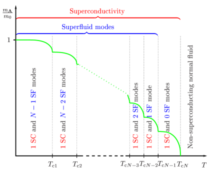
Figure 12: (Color online). Phase transitions in the $N$-flavor London superconductor with different bare stiffnesses of the $N$ order parameter components. The green line is the gauge field mass $m_{\mathbf{A}}$. At the highest temperature the system becomes superconducting via a phase transition in the inverted 3D$xy$ universality class. At the lower transitions the system develops composite neutral superfluid modes in the superconducting state via a series of $N-1$ phase transitions, all in the 3D$xy$ universality class.

Summarizing the previous two sections, the resulting schematic phase diagram of the $N$-flavor London superconductor in the absence of external field is presented in Fig. 12. Assuming the bare stiffnesses have been chosen to have well separated bare energy scales associated with the twist of phases of every flavor, we find $N$ distinct critical points. At the highest critical temperature, the charged vortex mode condenses and the gauge field acquires a mass, driving the system into a superconducting phase. For lower critical temperatures, neutral vortex loops condense and the system develops superfluid modes. Hence, in zero magnetic field there are $N-1$ superfluid modes arising in a superconducting state.

VII $N=2$ system in an external magnetic field, lattice and sub-lattice melting, and metallic superfluidity

We next discuss the situation when the system is subjected to an external magnetic field. Two important aspects of the physics to be described below, are i) three dimensionality and ii) a significant difference in the bare stiffnesses of the condensates. As discussed recently BSA ; SSBS , when an external magnetic field is applied to a three dimensional type-II $N$-component superconductor, it changes its properties much more dramatically than in the ordinary $N=1$ case. The composite charged vortices have finite energy per unit length and couple to the magnetic field, and hence are relevant for magnetic properties. If the bare stiffnesses of the fields are different, the existence of composite purely charged vortices results in a particularly rich phase diagram with several novel phases and phase transitions. Note that in the following two chapters we denote a constituent vortex originating in a $2\pi$ phase-winding in $\theta^{(\alpha)}$ a type-$\alpha$ vortex, where $\alpha\in[1,\dots,N]$.

VII.1 $N=2$ system in external field at $T=0$

In the presence of an external magnetic field, but in the absence of thermal fluctuations, the formation of an Abrikosov lattice of non-composite vortices is forbidden because these defects have a logarithmically divergent energyfrac ; smiseth2004 , cf. discussion following Eq. (13). In a type-II $N$-component system, the system forms a lattice of composite vortices for which $\Delta\theta^{(\alpha)}=2\pi$ for every $\alpha\in[1,\dots,N]$. A schematic picture of the resulting lattice of composite vortices in an $N=2$ superconductor is shown in Fig. 13. In the discussion below we consider the type-II limit, but not extreme type-II since the interaction between vortices of different species is depleted at the length scales smaller than the penetration length, cf. Eq. (12) and the discussion following Eq. (13). We do not discuss effects of this depletion assuming a moderately short penetration length scale.

Figure 13: (Color online). A type-II, $N=2$ system at zero temperature in external magnetic field forms a lattice of composite Abrikosov vortices. A composite vortex may be viewed as co-centered type-1 (red) and type-2 (blue) vortices $(\Delta\theta^{(1)}=2\pi,\Delta\theta^{(2)}=2\pi)$.

VII.2 Effects of low-temperature fluctuations on field-induced composite vortices

In this subsection, we will consider the effects of thermal fluctuations, and how it affects the Abrikosov vortex lattice of composite vortices defined above.

VII.2.1 Thermal generation of loop-like splitting of line vortices

At finite temperature, the $N$-component system subjected to a magnetic field $\mathbf{B}$ will exhibit thermal excitations in the form of vortex loops with fractional flux similar to the ${\mathbf{B}}=0$ discussion in the first part of this paper. We observe that since the field-induced composite vortices are logarithmically bound frac ; smiseth2004 , thermal fluctuations will induce a local splitting of composite vortices in a configuration of two half-loops connected to a straight line BSA ; SSBS as shown in Fig. 14.

Figure 14: (Color online). Low-temperature fluctuations in the $N=2$ system subjected to a magnetic field. Thermal fluctuations generate closed loops of composite fractional flux vortices and local splitting of field-induced composite vortex lines. The type-1 vortices (red) are the vortices of the component with the lowest bare phase stiffness. When these vortices are viewed as world-lines of bosons, they constitute the “lighter” of the vortex species. These “light” vortices fluctuate more strongly than the “heavier” type-2 vortices (blue).

We observe that every branch of a “split loop” formed on a field-induced vortex line features neutral as well as charged vorticity. The interaction between these two branches is mediated by a neutral vortex mode exclusively associated with the phase difference $\gamma=\theta^{(1)}-\theta^{(2)}$. The screened charged mode does not contribute to the interaction between the two branches. This is implicit in Eq. (12) as follows. The vortex segments of different flavors do not interact at short distances much smaller than $\lambda=m_{0}^{-1}$, where the charge, or $m_{0}^{2}$ appearing in the interaction matrix Eq. (12), can be ignored. On such length scales, the screened part of the interaction matrix is essentially unscreened, and is canceled by the inter-flavor interaction, which is unscreened on all length scales. Hence, as also discussed in Section II, the intra-vortex interaction is strongly reduced at length scales smaller than $\lambda$.

Moreover, in terms of the field $\gamma=\theta^{(1)}-\theta^{(2)}$, two split branches of a composite field-induced vortex have opposite vorticities ($\Delta\gamma=2\pi$ on one branch and $\Delta\gamma=-2\pi$ on another branch). On the other hand, such a loop emits two integer flux vortices at its top and bottom, which do not feature neutral vorticity. So the process of such a thermal local splitting of a field-induced line may be mapped onto a thermally generated proliferation of closed vortex loops in the artificial phase field $\gamma$ as those in the neutral $N=1$ model in absence of magnetic field tesanovic1999 ; nguyen1999 . Hence, somewhat counterintuitively such a splitting transition should be in the 3D$xy$ universality class BSA ; SSBS . This transition, being topological in its origin, should not be confused with the topological Kosterlitz-Thouless transition known to occur in planar systems.

VII.2.2 Melting

Apart from the splitting of composite vortices and generation of closed vortex loops, the thermal fluctuations will produce one more competing process. That is, the lattice of composite vortices can be mapped onto an ordinary vortex lattice in a one-component superconductor. Sufficiently strong thermal fluctuations drive a first-order melting transition of the field-induced Abrikosov lattice Hetzel1992 ; Fossheim_Sudbo_book ; nguyen1999 . A counterpart to this effect for the case $N=2$ when $|\psi^{(1)}|\neq|\psi^{(2)}|$ is much more complicated. We next consider this process in the regimes of low and high magnetic fields, separately.

VII.3 Sublattice melting in low magnetic fields

Consider the case of weak magnetic field (much smaller than the upper critical magnetic field for which superconductivity is essentially destroyed) for the situation where $|\psi^{(1)}|\ll|\psi^{(2)}|$. Introducing a characteristic temperature associated with a melting of the type-2 vortex lattice in the absence of the condensate $\Psi_{0}^{(1)}$, then at sufficiently low magnetic field this melting temperature will be much higher than the characteristic temperature of thermal decomposition of a composite vortex line into two individual vortex lines. Thus, the first transition that would be encountered upon heating the system, is the thermal splitting of field-induced composite vortices into separate type-1 and type-2 vortices. This would be accompanied by a proliferation of closed loops of type-1 vortices, while the vortices of type-2 will remain arranged in a lattice. We will denote this phase transition as sublattice melting BSA ; SSBS . The critical temperature of this phase transition is denoted $T_{\rm SLM}$ (see Fig. 18). A schematic picture of the sublattice vortex liquid is given in Fig. 15. As discussed above, upon thermal decomposition of the composite vortices, the emerging individual vortices can be mapped onto positively and negatively electrically charged strings which logarithmically interact with each other.

Quite remarkably, the Abrikosov lattice order for the component with the highest phase stiffness survives the decomposition transition, for the following reason. The dominant interaction between individual vortices is the long-ranged interaction mediated by neutral vorticity, cf. Eq. (12). This permits a mapping of such vortices onto positively and negatively charged strings. Upon thermal decomposition, the effective long-range Coulomb interaction mediated by the neutral mode is screened without affecting the charged modes. Consider the case when $|\psi^{(1)}|\ll|\psi^{(2)}|$. Then the stiffness $|\psi^{(2)}|$ is large enough to keep the type-2 vortices arranged in a lattice while the stiffness $|\psi^{(1)}|$ is too weak to constrain type-1 vortices to the lattice. Thus, the “light” type-1 vortex lines are in their molten phase. This is the physical origin of the sublattice melting process. The situation is illustrated in Fig. 15. We emphasize that the existence of the regime of sublattice melting follows from the fact that the stiffness of the neutral mode, which keeps composite vortices bound at low temperatures, is always smaller than the smallest stiffness of the individual condensates, namely

$$J_{\rm neutral}=\frac{|\psi^{(1)}|^{2}|\psi^{(2)}|^{2}}{|\psi^{(1)}|^{2}+|\psi^{(2)}|^{2}}<|\psi^{(1)}|^{2}.$$ (56)

Figure 15: (Color online). A vortex liquid of type-1 vortices (red) immersed in a background of a type-2 vortex lattice (blue) in the $N=2$ system in the regime $|\psi^{(1)}|\ll|\psi^{(2)}|$. This is the type-1 vortex sublattice melting. There is a temperature region in low magnetic field when “light” vortices are decoupled and form a liquid. “Light” vortex loops are proliferated, while “heavy” vortices form a lattice immersed a liquid of “heavy” vortex loops. Both heavy and light vortices carry only a fraction of magnetic flux quantum in this state.

VII.4 Composite vortex lattice melting in strong magnetic fields

It is known from the $N=1$ system that an increase in magnetic field suppresses the melting temperature of the vortex latticeFossheim_Sudbo_book . Thus, an important and characteristic feature of the phase diagram of the $N=2$ system is that the composite vortex lattice melting curve should at some point cross the decomposition curve. Thus, the phase diagram should feature a composite vortex liquid phase in the low-temperature, high-magnetic field corner. A schematic picture of this phase is given in Fig. 16

Figure 16: (Color online). Liquid of composite vortices in the $N=2$ model immersed in a liquid of non-proliferated vortex loops. It is realized for $|\psi^{(1)}|\ll|\psi^{(2)}|$ in strong magnetic fields.

VII.5 Vortex line plasma in the $N=2$ model

If the temperature is raised either at strong or weak magnetic fields, a situation arises where all field-induced composite vortices are decomposed and disordered. In addition, closed loops have proliferatedtesanovic1999 ; nguyen1999 ; Fossheim_Sudbo_book . A schematic picture of this state is shown in Fig. 17.

Figure 17: (Color online). Plasma of fractional vortices in the $N=2$ model in the regime $|\psi^{(1)}|\ll|\psi^{(2)}|$ at high temperatures.

The resulting phase diagram of the $N=2$ GL model featuring the various transitions described above, is shown in Fig. 18.

Figure 18: (Color online). A schematic phase diagram of different phases of vortex matter and phase transition lines in the $N=2$ model in the regime $|\psi^{(1)}|\neq|\psi^{(2)}|$. At temperatures $T_{\rm M}^{\rm c}$, $T_{\rm M}^{\rm 2}$, and $T_{\rm SLM}$ the melting of the composite vortex lattice, the sublattice of heavy vortices and the sublattice of the light vortices occurs, respectively. At $T_{\rm LP}$ the composite vortices decompose. The temperatures $T_{\rm L}^{\rm 1}$ and $T_{\rm L}^{\rm 2}$ denote temperatures where a phase transition via a proliferation of vortex loops would take place in the absence of a magnetic field in models with bare phase stiffnesses $|\tilde{\psi}^{(\alpha)}|(T)$ equal to $|\psi^{(\alpha)}|(B,T)$ (where $\alpha=1,2$), if the effect of a magnetic were to be taken into account only via the depletion of the modulus of the order parameter.

VII.6 Physical interpretation of the external field-induced phases of the $N=2$ model

We next discuss the physical interpretation of the various phases that appear as a result of the above described vortex matter transitions. The resulting phases, which exhibit some quite unusual properties, come about as a result of the interplay between the topology of the system and thermal fluctuations. This is rather remarkable, given the three-dimensionality of the systems we consider.

VII.6.1 Vortex lattice melting and the disappearance of superconductivity.

Consider first the melting transition of an interacting ensemble of composite Abrikosov vortices. This phase transition, which is of first order Hetzel1992 , corresponds to the lines $T_{\rm M}^{\rm c}(B)$ and $T_{\rm M}^{2}(B)$ shown in Fig. 18. It is only the gauge-charged mode that couples to the external field, while the neutral mode does not. The charged mode at low temperature forms an Abrikosov vortex lattice with a melting temperature that is suppressed with increasing magnetic field Nelson1988 ; Houghton1989 ; Blatter1994 ; Fossheim_Sudbo_book . The melting temperature of the Abrikosov vortex lattice can be suppressed below the temperature where the neutral mode proliferates and where the composite vortex lines decompose. For $N=1$, it is known that when the Abrikosov lattice melts, superconductivity is lost also along the direction of the magnetic field Nonomura1998 ; nguyen1999 . The situation in the $N=2$ model is much more complex, since then there still exists a superfluid mode (the gauge neutral mode) which is decoupled from external magnetic field. Thus, upon melting of the Abrikosov lattice we arrive at emergent effective neutral superfluidity existing in a system of charged particles BSA . This is a genuinely novel state of condensed matter, and moreover one which should be realizable in liquid metallic states of light atoms at in principle experimentally accessible pressures in the range of $400{\rm GPa}$ BSA .

So in the absence of an external magnetic field, the system thermally excites only fractional flux vortices in the forms of loops, with phase windings only in individual condensates, and these fluctuations are responsible for critical properties. In contrast, the purely charged vortices (i.e. the composite one-flux-quantum vortices with no neutral super-flow) are not relevant in the absence of external field and the system is either a superconductor (below $T_{\rm c2}$) or a superconductor with neutral mode (below $T_{\rm c1}$). Thus, the effect of a sufficiently strong magnetic field essentially inverts the temperatures of the transitions by melting the lattice of charged modes at $T_{\rm M}^{\rm c}(B)$ while leaving neutral modes intact.

The phase transition from a superconducting superfluid phase where the neutral mode is superfluid and the Abrikosov vortex lattice is intact such that longitudinal superconductivity (parallel to the magnetic field) existsnguyen1999 ; Nonomura1998 , to a metallic superfluid phase where the system is superfluid, but longitudinal superconductivity is lost due to the melting of the vortex lattice, can be mapped onto a lattice melting transition in the $N=1$ model , because it is governed only by composite vortices and neutral modes are not involved. Thus it is a first order phase transition Hetzel1992 ; Fossheim_Sudbo_book .

VII.6.2 Decomposition. The disappearance of superfluidity.

Analogously, the physical meaning of the sublattice melting transition $T_{\rm SLM}$ (see Fig. 18) is a transition from a superconducting superfluid to an ordinary one-gap superconductor, because a disordering of the phase $\theta^{(1)}$ destroys the massless neutral boson associated with the gauge invariant phase difference $\theta^{(1)}-\theta^{(2)}$.

If we heat the system further, the ordinary superconductivity will disappear via disordering of the phase $\theta^{(2)}$ when we reach the melting transition of the remaining sublattice of “heavy” vortices at $T_{\rm M}^{2}$.

The system features one more phase transition. That is a transition from the metallic superfluid to a normal fluid, which has a purely topological origin. That is, from the vortex matter point of view, this manifests itself as a decomposition of a liquid of composite vortices to a “plasma” of individual vortices at the characteristic temperature $T_{\rm LP}$, and such a transition has no counterpart in an $N=1$ superconductor. A schematic diagram of the resulting physical phases is shown in Fig. 19.

Figure 19: (Color online). A schematic phase diagram of physical states appearing in the $N=2$ model in the regime $|\psi^{(1)}|\neq|\psi^{(2)}|$ as a consequence of vortex matter phase transitions. Increasing the magnetic field suppresses the melting transition of the composite vortex lattice formed by the charged mode below the proliferation line for the neutral mode, which does not couple to magnetic field. In the absence of disorder (pinning of vortices), superconductivity only remains along the direction of the magnetic field, provided that the vortex system remains in a lattice phase. When the composite vortex lattice melts, the system looses ability to carry dissipation-less charge currents, but at large enough magnetic field, the neutral mode should still be superfluid above the melting temperature BSA . Thus, we have a first order phase transition from a superconducting superfluid to a metallic superfluid. The neutral mode proliferates through a second order phase transition in the 3D$xy$ universality class. Therefore, at large enough magnetic fields, a 3D$xy$ anomaly in the specific heat should appear inside the vortex liquid phase. The separation between the first order specific heat anomaly due to vortex lattice melting and the 3D$xy$ anomaly due to loop-proliferation should increase with increasing magnetic field. At low magnetic fields one has another phase transition inside the Abrikosov vortex lattice phase, from a superconducting superfluid to a one-gap (“ordinary”) superconducting state.

VII.6.3 A direct SSF $\to$ NSF transition

We note also the possibility of an existence of a phase transition directly from a superconducting superfluid (SSF) to a metallic normal fluid (NF), shown in Fig. 20.

Figure 20: (Color online). A direct phase transition from SSF to NF phase (shown with red arrow).

What is remarkable is that this resembles (while indeed being a different type of transition) the type of direct phase transition from a low temperature phase with Higgs mass and superfluid density of the neutral mode, to a phase with zero Higgs mass and zero helicity modulus of the neutral mode that we would find in zero magnetic field when the bare phase stiffnesses of Eq. (1) are equal, i.e. $|\psi^{(1)}|=|\psi^{(2)}|$   sachdev2004 ; motrunich2004 ; smiseth2004 . The SSF phase features one massless dual Higgs photon, and one massive Higgs photon while the NF phase features one massless photon and one massive dual Higgs photon. These phases are therefore self-dual, in analogy to the situation encountered when Eq. (1) is viewed as a quantum anti-ferromagnet with easy-plane anisotropy sachdev2004 ; motrunich2004 . However, there is a significant difference. The novel critical point encountered in the case of the quantum antiferromagnet was a result of a superposition of a 3D$xy$ and an inverted 3D$xy$ critical point. In the $2$-flavor London model in finite magnetic field, the crossing point is a superposition between a 3D$xy$ critical line and first order phase transition line, so it should have a different character than the self-dual critical point discussed in Ref. motrunich2004, . It can, however, not be a 3D$xy$ or inverted 3D$xy$ critical point, since neither of these are critical points between self-dual phases.

Thus, both for high and low magnetic fields we have genuinely novel physics in that for a three dimensional system, i) a critical phenomenon takes place inside either the vortex liquid phase (high magnetic fields) or the vortex lattice phase (low magnetic fields), and ii) we have three new equilibrium states which have no counterpart in the $N=1$ case. Moreover, by the discussion given above, it is clear that the crossing point between the vortex lattice melting line and the neutral mode proliferation line warrants further study. This is best left for a separate computational analysis.

VII.7 Monte-Carlo results, finite magnetic field, $N=2$

We now present large-scale Monte Carlo results for the case $N=2$ in finite magnetic field at low magnetic fields when the temperature is varied SSBS . We consider the model based on Eq. (1) for $N=2$ on an $L^{3}$ lattice (with $L$ up $96$) with periodic boundary conditions for coupling constants $|\psi^{(1)}|^{2}=0.2$, $|\psi^{(2)}|^{2}=2$, and $e^{2}=1/10$. The ratio $|\psi^{(2)}|^{2}/|\psi^{(1)}|^{2}=10$ brings out one second order phase transition at $T_{\rm SLM}(B)$ in the 3D$xy$ universality class well below the melting temperature $T_{\rm M}^{2}$ of the vortex lattice. In LMH $|\psi^{(2)}|^{2}/|\psi^{(1)}|^{2}\approx 2000$, but the physical picture remains. For real estimates of $T_{\rm{SLM}}$ and $T_{\rm M}^{2}$ in LMH, see Ref. Ashcroft1999, . The Metropolis algorithm with local updating is used in combination with Ferrenberg-Swendsen reweighting. The external magnetic field $\mathbf{B}$ studied is $B^{x}=B^{y}=0$, $B^{z}=2\pi/32$, thus there are $32$ plaquettes in the $(x,y)$-plane per flux-quantum. This is imposed by splitting the gauge field into a static part $\mathbf{A}_{0}$ and a fluctuating part $\mathbf{A}_{\rm fluct}$. The former is kept fixed to $(A_{0}^{x},A_{0}^{y}(\mathbf{r}),A_{0}^{z})=(0,2\pi xf,0)$ where $f=1/32$ is the magnetic filling fraction, on top of which the latter field is free to fluctuate. Together with periodic boundary conditions on $\mathbf{A}_{\rm fluct}$, the constraint $\oint_{C}(\mathbf{A}_{0}+\mathbf{A}_{\rm fluct})d\mathbf{l}=2\pi fL^{2}$, where $C$ is a contour enclosing the system in the (x,y)-plane, is ensured. It is imperative to fluctuate $\mathbf{A}$, otherwise type-$1$ and type-$2$ vortices do not interact frac ; smiseth2004 . To investigate the transition at $T_{\rm{SLM}}$ we have performed finite size scaling (FSS) of the third moment of the action. The simulations are done by using vortices directly smiseth2004 , but with a finite magnetic induction $B^{z}=2\pi/32$.

We compute the specific heat $C_{V}$ and the third moment of the action. To probe the structural order of the vortex system we compute the planar structure function $S^{(\alpha)}(\mathbf{k}_{\perp})$ of the local vorticity $\mathbf{n}^{(\alpha)}(\mathbf{r})=\left(\mathbf{\nabla}\times\left[\mathbf{\nabla}\theta^{(\alpha)}-e~{}\mathbf{A}\right]\right)/2\pi$, given by

$$S^{(\alpha)}(\mathbf{k}_{\perp})=\frac{1}{(fL^{3})^{2}}~{}\langle|\sum_{\mathbf{r}}~{}n_{z}^{(\alpha)}(\mathbf{r})~{}e^{i\mathbf{k}_{\perp}\cdot\mathbf{r}_{\perp}}|^{2}\rangle,$$ (57)

where $\mathbf{r}$ runs over dual lattice sites and $\mathbf{k}_{\perp}$ is perpendicular to $\mathbf{B}$. This function will exhibit sharp peaks for the characteristic Bragg vectors $\mathbf{K}$ of the type-$\alpha$ vortex lattice and will feature a ring-structure in its corresponding liquid of type-$\alpha$ vortices. The signature of vortex sub-lattice melting will be a transition from a six-fold symmetric Bragg-peak structure to a ring structure in $S^{(1)}(\mathbf{K})$ while the peak structure remains intact in $S^{(2)}(\mathbf{K})$. Furthermore, we compute the vortex co-centricity $N_{\rm{co}}$ of type-$1$ and type-$2$ vortices, defined as $N_{\rm co}\equiv N^{+}_{\rm{co}}-N^{-}_{\rm{co}}$, where

$$N^{\pm}_{\rm{co}}\equiv\frac{\sum_{\mathbf{r}}|n_{z}^{(2)}(\mathbf{r})|\delta_{n_{z}^{(1)}(\mathbf{r}),\pm n_{z}^{(2)}(\mathbf{r})}}{\sum_{\mathbf{r}}|n_{z}^{(2)}(\mathbf{r})|},$$ (58)

where $\delta_{i,j}$ is the Kronecker-delta. The reason for considering $N_{\rm co}$ is that we then eliminate the effect of random overlap of vortices in the high-temperature phase $T>T_{\rm SLM}$ due to vortex-loop proliferation, and focus on the compositeness of field-induced vortices.

The quantity $N_{\rm{co}}$ is the fraction of type-$2$ vortex segments that are co-centered with type-$1$ vortices, providing a measure of the extent to which vortices of type-$1$ and type-$2$ form a composite vortex system. Hence, it probes the splitting processes visualized in Fig. 14. The results are shown in Fig. 21.

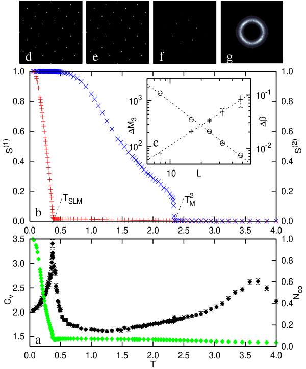
Figure 21: (Color online). MC results for $N=2$ $|\psi^{(1)}|^{2}=0.2$, $|\psi^{(2)}|^{2}=2$, and $e=1/\sqrt{10}$. Panel a: $C_{V}$ (black) and $N_{\rm co}$ (green). The $C_{V}$-anomaly at $T_{\rm{SLM}}=0.37$, where type-$1$ vortices proliferate, matches the point at which $N_{\rm co}$ drops to zero. Thus, type-$1$ vortices are torn off type-$2$ vortices. The remnant of the zero-field anomaly in $C_{V}$ is seen as a hump at $T\sim 3.6$. Panel b: $S^{(1)}(\mathbf{K})$ (red) and $S^{(2)}(\mathbf{K})$ (blue) for the particular Bragg vector $\mathbf{K}=(\pi/4,-\pi/4)$. $S^{(1)}(\mathbf{K})$ vanishes continuously at $T_{\rm{SLM}}$, while $S^{(2)}(\mathbf{K})$ vanishes discontinuously at $T_{\rm M}^{2}=2.34$. Panel c: FSS plots of the $M_{3}$ from which the exponents $\alpha=-0.02\pm 0.05$ and $\nu=0.67\pm 0.03$ is extracted, showing that the sub-lattice melting is a 3D$xy$ phase transition. Panels d, e, f, and g: plots of $S^{(2)}(\mathbf{k}_{\perp})$ for the temperatures $T_{\rm d}=0.35$, $T_{\rm e}=0.4$, $T_{\rm f}=1.66$, and $T_{\rm g}=2.85$, respectively. At $T_{\rm d}$, $T_{\rm e}$, and $T_{\rm f}$, the vortex lattice remains intact. The vortex lattice melts at $T_{\rm M}^{2}$ to give a vortex liquid ring pattern at $T_{\rm g}$.

At $T_{\rm{SLM}}$, $C_{V}$ has a pronounced peak associated with the 3D$xy$ transition, and a broader less pronounced peak which is the finite field remnant of the zero-field inverted 3D$xy$ transition nguyen1999 . Scaling of $M_{3}$ at $T_{\rm{SLM}}$ shown in the inset c in Fig. 21 yields the critical exponents $\alpha=-0.02\pm 0.05$ and $\nu=0.67\pm 0.03$ in agreement with the 3D$xy$ universality class. A novel result is that $S^{(1)}(\mathbf{K})$ vanishes continuously as the temperature approaches $T_{\rm{SLM}}$ from below, precisely the hallmark of the decomposition transition that separates the two types of vortex states depicted in Figs. 14 and 15. A related feature is the vanishing of $N_{\rm co}$ at $T_{\rm{SLM}}$ as a function of temperature, discussed in detail below. The first-order melting transition takes place at $T_{\rm M}^{2}$, where $S^{(2)}(\mathbf{K})$ vanishes discontinuously. This is the temperature at which the translational invariance is restored through melting of the type-$2$ vortex lattice. In the temperature interval $T<T_{\rm{SLM}}$ the system features superconductivity and superfluidity simultaneously BSA , since there is long-range order both in the charged and the neutral vortex modes. In the temperature interval $T_{\rm{SLM}}<T<T_{\rm M}^{2}$ long-range order in the neutral mode is destroyed by loop-proliferation of type-$1$ vortices, hence superfluidity is lost BSA . However, longitudinal one-component superconductivity is retained along the direction of the external magnetic field. For $T>T_{\rm M}^{2}$ superconductivity is also lost, hence this is the normal metallic state, which is a two-component vortex liquid.

The most unusual and surprising feature is the continuous variation of $S^{(1)}(\mathbf{K})$ with temperature, even at $T_{\rm{SLM}}$ where it vanishes. The explanation for this is the proliferation of type-$1$ vortices (which destroys the neutral superfluid mode) in the background of a composite vortex lattice, which the type-$1$ vortices essentially do not see, cf. Fig. 22. As far as the composite neutral Bose field $\theta^{(1)}-\theta^{(2)}$ is concerned, it is precisely as if the composite vortex lattice were not present at all. Hence, $S^{(1)}(\mathbf{K})$ vanishes for a completely different reason than $S^{(2)}(\mathbf{K})$, namely due to critical fluctuations, i.e. vortex-loop proliferation in the condensate component with lowest bare stiffness. Such a phase transition does not completely restore broken translational invariance associated with a vortex lattice, since for the type-$2$ vortices quite remarkably, the vortex lattice order survives the decomposition transition, due to interaction between heavy vortices mediated by charged modes. The vanishing of $N_{\rm{co}}$ is particularly interesting, and finds a natural explanation within the framework of the above discussion. That is, for $T\ll T_{\rm{SLM}}$, we have $N_{\rm{co}}\approx 1$, so the vortex system consists practically exclusively of composite vortices. As the temperature increases, thermal fluctuations induce excursions such as those illustrated in in Fig. 22, which reduces $N_{\rm co}^{\rm{+}}$ from its low-temperature value, reaching a minimum at $T_{\rm{SLM}}$ and then increase for $T>T_{\rm{SLM}}$.

We may view the splitting process as a type-$1$ closed vortex loop superposed on a vortex lattice of (slightly) fluctuating composite vortices. An important point to notice is that a type-$\alpha$ vortex does not interact with a composite vortex by means of a neutral mode. This follows from a topological argument that two split branches will feature nontrivial winding in the composite neutral field $\theta^{(1)}-\theta^{(2)}$, while a composite vortex line does not. Hence, the splitting transition may be viewed as a type-$1$ vortex loop-proliferation in a neutral superfluid. This is illustrated in Fig. 22.

Figure 22: (Color online). Detailed illustration of the low-temperature thermal fluctuations in a vortex lattice of composite vortices. A local excursion of a type-$1$ vortex away from the composite vortex lattice may be viewed as a type-$1$ bound vortex loop superposed on the composite vortex lattice. The composite vortex line does not interact with a vortex with nontrivial winding in $\Delta\gamma=\Delta(\theta^{(1)}-\theta^{(2)})$. A splitting of the composite vortex lattice may be thus viewed as a zero-field vortex-loop proliferation of type-$1$ vortices; a 3D$xy$ phase transition universality tesanovic1999 ; nguyen1999 ; Fossheim_Sudbo_book .

Thus, we may utilize the well-known results for the critical properties of the 3D$xy$ model for neutral superfluids described as a vortex-loop proliferation tesanovic1999 ; nguyen1999 ; Fossheim_Sudbo_book . This “vortex sublattice melting” phase transition is therefore in the 3D$xy$ universality class tesanovic1999 ; nguyen1999 ; Fossheim_Sudbo_book , not a first order melting transition. The resulting phase is one where superfluidity is lost and longitudinal superconductivity retained in the component $\Psi_{0}^{(2)}$.

Conversely, $N_{\rm co}^{\rm{-}}$ remains essentially zero until $T_{\rm{SLM}}$, thereafter increasing monotonically. For temperatures above, but close to $T_{\rm{SLM}}$, fluctuations in vortices originating in $\Delta\theta^{(2)}$ are still small, so the variations in $N_{\rm{co}}=N_{\rm co}^{\rm{+}}-N_{\rm co}^{\rm{-}}$ reflect thermal fluctuations in vortices originating in $\Delta\theta^{(1)}$. The increase of $N_{\rm co}^{\rm{\pm}}$ means that type-$1$ vortex loops are thermally generated, and thus tend to randomly overlap more with the moderately fluctuating type-$2$ vortices. At their first order melting transition, type-$2$ vortices fluctuate only slightly. Thus, the vanishing of $N_{\rm{co}}$ above $T_{\rm{SLM}}$ reflects the increase in the density of thermally generated type-$1$ vortex loops in the background of a slightly fluctuating type-$2$ vortex lattice.

VII.8 Graphical representation of phase disordering transitions in the $N=2$ model.

In Fig. 23 we present a schematic picture of configuration of the order parameters phases $\theta^{(1)}$ and $\theta^{(2)}$ in various points in physical space, when vortex matter drives the system into one of the above discussed superconducting and superfluid states.

Figure 23: (Color online). Phases of the order parameters in the various states for $N=2$. In the upper left panel, both $\theta^{(1)}$ and $\theta^{(2)}$ are ordered, this is the superconducting superfluid state. In the upper right panel, neither of the phases $\theta^{(1)}$ and $\theta^{(2)}$ are ordered, however the combination $\theta^{(1)}-\theta^{(2)}$ exhibits long-range order, this is the metallic superfluid state. In the lower left panel, $\theta^{(1)}$ is disordered and $\theta^{(2)}$ is ordered. In this case, the neutral superfluid mode is destroyed and we are left with one charged superconducting mode, this is the analog of the one-gap superconducting state. In the lower right panel, neither of the phases $\theta^{(1)}$ and $\theta^{(2)}$ are ordered and the combination $\theta^{(1)}-\theta^{(2)}$ does not exhibit long-range order, this is the metallic normal fluid state. The states illustrated in the upper left and lower right and left panels exist at zero as well as finite magnetic fields. The state illustrated in the upper right panel only exists at finite magnetic fields.

VIII The $N>2$ model in external magnetic field

We next consider the novel features that are encountered, compared to the $N=1$- and $N=2$ cases, when an $N>2$ system is subjected to an external magnetic field. The new features are due to the fact that we have more than one neutral vortex mode, and that a vortex with phase winding in any single phase field $\theta^{(\alpha)}$ will excite $N-1$ neutral modes (see Appendix A). We consider first the case $N=3$, followed by the case $N=4$. En route we introduce the useful concept of “color charge” which facilitates a discussion of the universality class of the phase transitions that occur in multi-component superconductors in external magnetic field when composite vortices decompose due to thermal fluctuations.

VIII.1 Decomposition transitions, $N=3$

We stress that the system is not mapped onto a $U(1)\times U(1)$ neutral system because the neutral modes remain topologically coupled, as a consequence of multiple connectedness of space introduced by the vortex core. It manifests itself in the fact that any single phase variable $\theta^{(\alpha)};\alpha\in[1,2,3]$ excites two neutral modes, as illustrated in detail below.

We introduce bare phase stiffnesses for the neutral modes in Eq. (53) as follows

$$J^{12} = \frac{|\psi^{(1)}|^{2}|\psi^{(2)}|^{2}}{\Psi^{2}},$$

$$J^{23} = \frac{|\psi^{(1)}|^{2}|\psi^{(3)}|^{2}}{\Psi^{2}},$$

$$J^{13} = \frac{|\psi^{(2)}|^{2}|\psi^{(3)}|^{2}}{\Psi^{2}}.$$ (59)

Hence, a vortex with phase windings $(\Delta\theta^{(1)}=2\pi,\Delta\theta^{(2)}=0,\Delta\theta^{(3)}=0)$, can be mapped onto two co-centered vortices in a two-component neutral superfluid with bare stiffnesses $J^{12}$ and $J^{13}$. Thus, at a distance larger than the penetration length, such a vortex interacts with a vortex $(\Delta\theta^{(1)}=-2\pi,\Delta\theta^{(2)}=0,\Delta\theta^{(3)}=0)$ like two vortices in a neutral superfluid with bare phase stiffness $\tilde{J}=J^{12}+J^{13}$.

Intra-vortex interaction, e.g. of the vortex $(\Delta\theta^{(1)}=2\pi,\Delta\theta^{(2)}=0,\Delta\theta^{(3)}=0)$ with a vortex $(\Delta\theta^{(1)}=0,\Delta\theta^{(2)}=2\pi,\Delta\theta^{(3)}=0)$ or with a vortex $(\Delta\theta^{(1)}=0,\Delta\theta^{(2)}=0,\Delta\theta^{(3)}=2\pi)$ is more complicated. It can most conveniently be described by introduction of the “color charge” concept, which we explain in the next subsection, VIII.2.

First, however, we observe that only a composite vortex $(\Delta\theta^{(1)}=2\pi,\Delta\theta^{(2)}=2\pi,\Delta\theta^{(3)}=2\pi)$ has finite energy. The key feature of a system with $|\psi^{(1)}|\neq|\psi^{(2)}|\neq|\psi^{(3)}|$, is that the three elementary constituent vortices are bound with different strength to such a composite vortex. For example, when $|\psi^{(1)}|\ll|\psi^{(2)}|\ll|\psi^{(3)}|$, the neutral modes excited by a vortex $(\Delta\theta^{(1)}=2\pi,\Delta\theta^{(2)}=0,\Delta\theta^{(3)}=0)$ have bare phase stiffnesses $(J^{12},J^{13})\ll J^{23}$. This in turn implies that in the composite vortex $(\Delta\theta^{(1)}=2\pi,\Delta\theta^{(2)}=2\pi,\Delta\theta^{(3)}=2\pi)$, the constituent elementary vortex $(\Delta\theta^{(1)}=2\pi,\Delta\theta^{(2)}=0,\Delta\theta^{(3)}=0)$ is most loosely bound. Thus, in contrast to the $N=2$ case, the effect of thermal fluctuations for $N=3$ is a two step transition. In the general $N$ case the process of stripping a composite vortex of its $N$ constituent vortices is an $N-1$-step process occurring successively, starting at $T_{\rm c1}$ and progressing up through $T_{\rm c2}$ up to $T_{{\rm c}N-1}$, at which point the vortex system is fully decomposed.

For $N=3$, at a low temperature determined by the smallest bare phase stiffness $|\psi^{(1)}|$ and by $J^{12}$ and $J^{13}$, there should therefore take place a partial decomposition of the vortex $(\Delta\theta^{(1)}=2\pi,\Delta\theta^{(2)}=2\pi,\Delta\theta^{(3)}=2\pi)$ into two vortices $(\Delta\theta^{(1)}=2\pi,\Delta\theta^{(2)}=0,\Delta\theta^{(3)}=0)+(\Delta\theta^{(1)}=0,\Delta\theta^{(2)}=2\pi,\Delta\theta^{(3)}=2\pi)$, illustrated in Fig. 24. Then, upon increasing the temperature there should take place a phase transition, also illustrated in Fig. 24, into a fully decomposed state defined by the phase windings $(\Delta\theta^{(1)}=2\pi,\Delta\theta^{(2)}=0,\Delta\theta^{(3)}=0)+(\Delta\theta^{(1)}=0,\Delta\theta^{(2)}=2\pi,\Delta\theta^{(3)}=2\pi)\to(\Delta\theta^{(1)}=2\pi,\Delta\theta^{(2)}=0,\Delta\theta^{(3)}=0)+(\Delta\theta^{(1)}=0,\Delta\theta^{(2)}=2\pi,\Delta\theta^{(3)}=0)+(\Delta\theta^{(1)}=0,\Delta\theta^{(2)}=0,\Delta\theta^{(3)}=2\pi)$.

Figure 24: (Color online). A two-step decomposition transition in the $N=3$ model in external magnetic field. The “lightest” vortex component, originating in the order parameter component with the lowest bare phase stiffness, tears itself loose from the composite Abrikosov vortex of the two stiffer order parameter components at $T_{\rm Spl}^{1}$. At a higher temperature $T_{\rm Spl}^{2}$, the “next-to-lightest” vortex component (green vortex), originating in the order parameter component with the next-to-lowest bare phase stiffness, tears itself loose from the vortex of the stiffest order parameter component in the background of proliferated vortices originating in non-trivial phase-windings of the phase with lowest phase stiffness (red vortex).

We also stress that apart from the neutral mode $(\theta^{(2)}-\theta^{(3)})$, which provides an attractive interaction for the vortex pair $(\Delta\theta^{(1)}=0,\Delta\theta^{(2)}=2\pi,\Delta\theta^{(3)}=0)+(\Delta\theta^{(1)}=0,\Delta\theta^{(2)}=0,\Delta\theta^{(3)}=2\pi)$, the first of these vortices excites the neutral mode $(\theta^{(1)}-\theta^{(2)})$ which consists of oppositely directed currents in the condensates $\Psi_{0}^{(1)}$ and $\Psi_{0}^{(2)}$. The second vortex excites the mode $(\theta^{(1)}-\theta^{(3)})$ which is associated with oppositely directed currents in condensates $\Psi_{0}^{(1)}$ and $\Psi_{0}^{(3)}$. These modes, apart from giving the pair $(\Delta\theta^{(1)}=0,\Delta\theta^{(2)}=2\pi,\Delta\theta^{(3)}=0)+(\Delta\theta^{(1)}=0,\Delta\theta^{(2)}=0,\Delta\theta^{(3)}=2\pi)$ logarithmically divergent energy per unit lengthfrac ; smiseth2004 , also yield some repulsive interaction in this pair, because both the modes $(\theta^{(1)}-\theta^{(2)})$ and $(\theta^{(1)}-\theta^{(3)})$ feature unscreened currents of condensate $\Psi_{0}^{(1)}$. However, such a repulsive interaction in this pair is negligibly small in the considered regime $|\psi^{(1)}|\ll|\psi^{(2)}|\ll|\psi^{(3)}|$, compared to the interactions mediated by the mode $(\theta^{(2)}-\theta^{(3)})$.

VIII.2 Color electric charge

Formally, the partial decomposition process can be described by introducing the concept of “color electric charges”. That is, we may introduce e.g. “+red”, “+green” and “+blue” charges associated with $2\pi$ windings in $(\theta^{(1)}-\theta^{(2)})$, $(\theta^{(1)}-\theta^{(3)})$ and $(\theta^{(2)}-\theta^{(3)})$, respectively (see Tab. 2). If we have a $-2\pi$ winding in $(\theta^{(1)}-\theta^{(2)})$, $(\theta^{(1)}-\theta^{(3)})$ or $(\theta^{(2)}-\theta^{(3)})$, that would correspond to “ $-$red”, “$-$green” and “$-$blue” color electric charges, respectively. We stress once more that in order to preserve single-valuedness of the order parameters, the $\pm 2\pi$ gains in phase differences may only come as $\pm 2\pi$ gains in individual phases. For example if we would have $(\Delta\theta^{(1)}=3\pi/4,\Delta\theta^{(2)}=-5\pi/4)$ then $(\theta^{(1)}-\theta^{(2)})$ would change by $2\pi$. However, such a configuration would be unphysical because individual order parameters $\Psi_{0}^{(1)}$ and $\Psi_{0}^{(2)}$ would loose their single-valuedness. Then, a vortex $(\Delta\theta^{(1)}=2\pi,\Delta\theta^{(2)}=0,\Delta\theta^{(3)}=0)$ which excites two neutral modes associated with $(\theta^{(1)}-\theta^{(2)})$ and $(\theta^{(1)}-\theta^{(3)})$ with stiffnesses $J^{12}$ and $J^{13}$, respectively, may be viewed as a color charged string with color charge “$+$red” and “$+$green”.

The regime $|\psi^{(1)}|\ll|\psi^{(2)}|\ll|\psi^{(3)}|$, i.e. when $J^{12}\ll J^{13}\ll J^{23}$, corresponds to the situation where red electric charges are much weaker than green charges, which in turn are much weaker than the blue charges. The blue charge then dominates the binding of the vortices $(\Delta\theta^{(1)}=0,\Delta\theta^{(2)}=2\pi,\Delta\theta^{(3)}=0)$ and $(\Delta\theta^{(1)}=0,\Delta\theta^{(2)}=0,\Delta\theta^{(3)}=2\pi)$. The tightly bound composite vortex $(\Delta\theta^{(1)}=0,\Delta\theta^{(2)}=2\pi,\Delta\theta^{(3)}=2\pi)$ then has electric charge $(-\rm{red},-\rm{green})$ which loosely binds it with $(+\rm{red},+\rm{green})$ color charged vortex $(\Delta\theta^{(1)}=2\pi,\Delta\theta^{(2)}=0,\Delta\theta^{(3)}=0)$ into a color charge neutral finite energy one-flux-quantum vortex $(\Delta\theta^{(1)}=2\pi,\Delta\theta^{(2)}=2\pi,\Delta\theta^{(3)}=2\pi)$.

In Fig. 25, we illustrate how to connect the vortex picture to the picture of color charges, for the case $N=3$. For $N=3$, each type of vortex is a bound state of two color charges.

Table 2: A color charge is defined as a $\pm 2\pi$ winding in the mode $(\theta^{(\alpha)}-\theta^{(\eta)})$ with the following mapping for $N=3$.

Mode:	$(\theta^{(1)}-\theta^{(2)})$	$(\theta^{(1)}-\theta^{(3)})$	$(\theta^{(2)}-\theta^{(3)})$
Color charge:	red	green	blue

Figure 25: (Color online). The connection between vortex illustrations and bound states of color charges, for the case $N=3$. Each type of vortex is a bound state of 2 color charges. The radius of each black circle is for graphical convenience is used to differentiate between “heavy” and “light” vortices. The order parameter component with the lowest bare phase stiffness is taken to be the vortex with the “smallest diameter”. A vortex originating in a non-trivial phase-winding in $\theta^{(\alpha)}$ is denoted a type-$\alpha$ vortex. The color of the vortex on the top of the Figure should not be confused with the color of the electric charges in the “dual” charge representation.

A schematic picture of the low-temperature composite vortex lattice phase, the partial decomposition transition in the color electric charge representation, and the complete decomposition transition, are given in Figs. 26, 28, and 29.

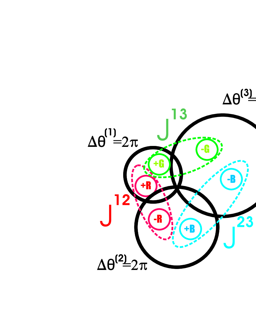
Figure 26: (Color online). A color charge representation for $N=3$ of the composite vortex lattice phase illustrated also in the left part of Fig. 24. This low-temperature phase, where the fluctuations of the composite vortex lines only involve small excursions of each of the constituent vortex lines away from the main composite object, may be viewed as a 3-color dielectric phase. The main composite vortex line is “anchored” on the thickest vortex. We assume we are at temperatures and fields such that the thickest vortex line does not undergo a melting transition. Each constituent vortex may be viewed as a bound state of certain combinations of color charges. The composite vortex line may, on the other hand, be viewed as bound states of $\pm{\rm red}$, $\pm{\rm green}$, and $\pm{\rm blue}$ charges, as indicated by the dotted ellipses. This is a three-color dielectric “insulating” phase. We strongly emphasize that the above illustration is meant to illustrate what the situation is in a typical cross section along the lines, which are not rigid straight vortex lines.

For the purposes of determining the universality class of this partial decomposition, which is a genuine phase transition, it may also be viewed as follows. The completely intact composite vortex is color charge neutral in the sense that it contains a positive and negative electric charge of each color. The fluctuation snapshot in the left part of Fig. 24 can be viewed as a completely intact composite vortex line with a small type-1 vortex loop superimposed on it as shown on Fig. 27.

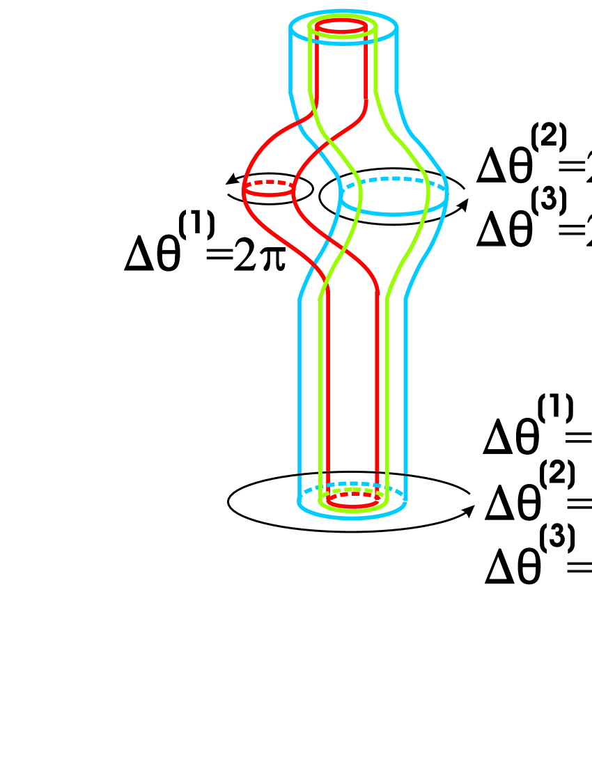
Figure 27: (Color online). A local thermally driven detachment of the type-$1$ vortex line (red color) from the composite vortex line can be viewed as a superposition of thermally created closed type-$1$ vortex loop on a completely composite vortex line. Both processes are topologically equivalent because the vorticity of the type-$1$ constituent vortex in the composite vortex line is exactly canceled by a superimposed type-$1$ vortex ring with the opposite vorticity. We stress that if left segment of a vortex loop has a counterclockwise vorticity then the opposite right segment has a clockwise vorticity.

The type-$1$ vortex loop which carries a red and green electric charges does not interact with the composite vortex which is color charge neutral. This can also be seen by examining the vortex interaction matrix given in Eq. (12). That is, when we add up the neutral-mode-mediated interactions between the type-$1$ vortex with all three type-$1,2,3$ vortices in the composite vortex $(\Delta\theta^{(1)}=2\pi,\Delta\theta^{(2)}=2\pi,\Delta\theta^{(3)}=2\pi)$ they add to zero. The situation in the right part of Fig. 24 is topologically equivalent to a completely intact composite vortex line superimposed with one segment of an unbound vortex loop. Therefore the transition may be viewed as an Onsager vortex loop proliferation transition Onsager1949 ; tesanovic1999 ; nguyen1999 of type-$1$ vortex loops in the background of a color charge neutral composite vortex lattice BSA ; SSBS . That is because type-$1$ vortex loops, from the point of view of superfluid modes, cannot “see” color charge neutral vortex lines, so this is equivalent to a type-$1$ vortex-loop proliferation transition in the complete absence of a composite color charge neutral vortex lattice. Since these vortices excite neutral modes, this transition, which is the first stage in decomposing a color charge neutral composite vortex line, is a vortex loop proliferation transition in the 3D$xy$ universality class BSA ; SSBS . In the color charge representation given in Fig. 28, this also means that the first-stage partial decomposition transition of three charged fluctuating line objects with different charges (but such that the algebraic sum of their charges add up to zero) is also a $2$-color metal-insulator phase transition in the 3D$xy$ universality class, involving flexible color line charges.

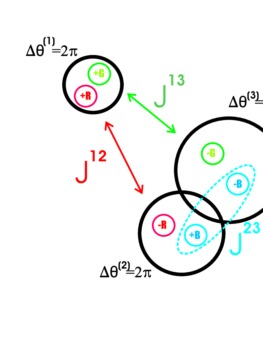
Figure 28: (Color online). A color charge representation for $N=3$ of the partial decomposition transition In the color charge representation, this may be viewed as a $\rm{red}$-$\rm{green}$ dielectric-metal transition, while the $\rm{blue}$ dielectric phase remains intact. As explained in the text, this partial 2-color metal-insulator transition involving fluctuating line charges, is in the 3D$xy$ universality class. The dotted ellipse indicates which color is involved in forming the remaining dielectric phase.

The usefulness of the color charge representation becomes particularly clear when we go on to describe the second stage of the decomposition transition, illustrated in Fig. 24. This transition may be viewed as a proliferation of type-$2$ vortex loops in the background of liberated type-$1$ vortex loops, all superimposed on a background composite vortex lattice. The situation therefore is more complicated than in the first stage illustrated in Fig. 24, since that was a proliferation of type-$1$ loops in vacuum.

However, let us view this transition in the color charge picture, illustrated in going from Fig. 28 to Fig. 29. This is a metal-insulator transition for the $\rm{blue}$-charge sector in the background of coexistent $\rm{red}$ and $\rm{green}$ metallic phases. However, $\rm{red}$ and $\rm{green}$ charges cannot screen $\rm{blue}$ charges, while these charges eliminate the neutral modes associated with them (that is the ones with bare stiffnesses $J^{12}$ and $J^{13}$). Therefore, this is a metal-insulator transition for the sector of the $\rm{blue}$ charges, while $\rm{red}$ and $\rm{green}$ charges screen themselves and do not affect this transition.

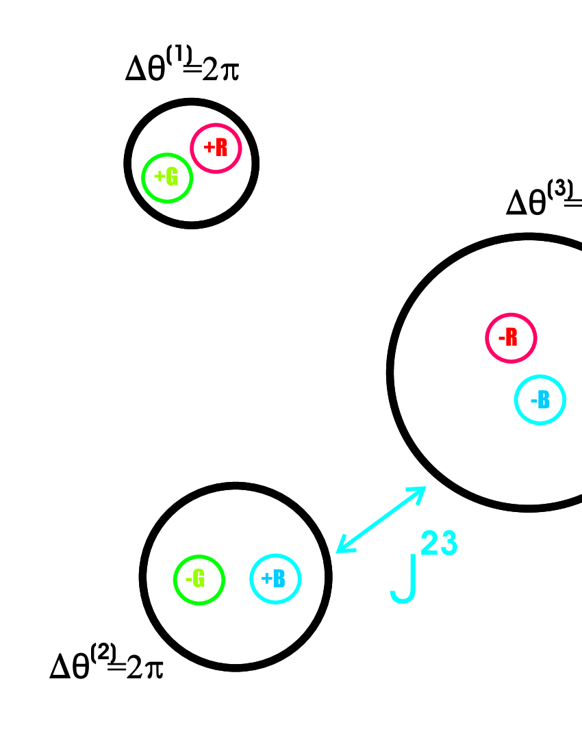
Figure 29: (Color online). A color charge representation of the complete decomposition transition also illustrated in Fig. 24. In the color charge representation, this may be viewed as a $\rm{blue}$ dielectric-metal transition, in the background of a $\rm{red}$-$\rm{green}$ metallic phase. As explained in the text, this complete “1-color” metal-insulator transition involving fluctuating line charges is in the same universality class as the partial decomposition transition, namely the 3D$xy$ universality class.

In the color charge representation given in Fig. 29, this also means that the second-stage decomposition transition depicted in Fig. 24 is a $1$-color metal-insulator transition in the 3D$xy$ universality class, involving flexible color charged strings.

VIII.3 Decomposition transitions, $N=4$

In Figs. 30, 31, 32, and 33 we illustrate the partial decomposition transitions for the case $N=4$ in the color charge picture. That is, we introduce as in the case $N=3$ case “$\pm$ red”, “$\pm$ green” and “$\pm$ blue” charges associated with $\pm 2\pi$ windings in $(\theta^{(1)}-\theta^{(2)})$, $(\theta^{(1)}-\theta^{(3)})$ and $(\theta^{(2)}-\theta^{(3)})$, respectively. In addition, we introduce “$\pm$ yellow”, “$\pm$ violet”, and “$\pm$ orange” charges associated with $\pm 2\pi$ windings in $(\theta^{(1)}-\theta^{(4)})$, $(\theta^{(2)}-\theta^{(4)})$ and $(\theta^{(3)}-\theta^{(4)})$, respectively (see Tab. 3). Therefore, the case $N=4$ features one new aspect which was absent in the case $N=3$, namely that for $N=4$ we need more color charges than number of order parameter components in order to completely cover all the possible ways that a neutral mode $(\theta^{(\alpha)}-\theta^{(\beta)})$ can be excited. Each type-$\alpha$ vortex is a bound state of three color charges, as indicated in Fig. 30.

The low-temperature phase is a $4$-composite color charge neutral vortex system, which may alternatively be viewed as a $6$-color dielectric phase, Fig. 30. The first-stage partial decomposition involves a type-$1$ vortex tearing itself off the $2$-composite vortex, i.e. a vortex loop proliferation of type-$1$ loops carrying $+\rm{red},+\rm{green},+\rm{yellow}$ color charges in the background of color charge neutral objects. So this is a phase transition in the 3D$xy$ universality class. It may alternatively be viewed as a $3$-color metal insulator transition in the $\rm{red},\rm{green},\rm{yellow}$ line-charge sectors, Fig. 31, leaving a $3$-color ($\rm{violet,blue,orange}$) dielectric phase. The second-stage decomposition process involves a type-$2$ vortex tearing itself off a $3$-composite vortex in the background of a system of proliferated type-$1$ loops. Due to screening of $\rm{red},\rm{green}$ and $\rm{yellow}$ charges, this transition may be viewed in a simplified manner. It may be considered as the first-stage decomposition in a $N=3$ system consisting of type-$2$, type-$3$, and type-$4$ vortices, involving $\rm{violet},\rm{blue}$, and $\rm{orange}$ charges. This we have already argued is a 3D$xy$ (type-$2$) vortex loop proliferation transition, when we considered the $N=3$ case. Alternatively, it may be viewed as a $2$-color metal-insulator transition in the $\rm{violet}$ and $\rm{blue}$ line-charge sectors, Fig. 32, leaving a $1$-color ($\rm{orange}$) dielectric phase. The third-stage decomposition may be viewed as a type-$3$ vortex loop proliferation in the background of type-$1$ and type-$2$ proliferated vortex lines. Due to screening of $\rm{violet}$ and $\rm{blue}$ charges this may be viewed in a simplified manner. It may be considered as a vortex loop proliferation of loops carrying $\rm{orange}$ charges in the background of an $\rm{orange}$-neutral vortex lattice, or vacuum. This is a vortex loop proliferation in the 3D$xy$ universality class BSA ; SSBS . Alternatively, it may be viewed as a $1$-color ($\rm{orange}$) metal-insulator transition, (see Fig. 33), leaving the $6$-color dielectric phase completely destroyed.

Table 3: A color charge is defined as a $\pm 2\pi$ winding in the mode $(\theta^{(\alpha)}-\theta^{(\eta)})$ with the following mapping for $N=4$.

Mode:	$(\theta^{(1)}-\theta^{(2)})$	$(\theta^{(1)}-\theta^{(3)})$	$(\theta^{(2)}-\theta^{(3)})$
Color charge:	red	green	blue
Mode:	$(\theta^{(1)}-\theta^{(4)})$	$(\theta^{(2)}-\theta^{(4)})$	$(\theta^{(3)}-\theta^{(4)})$
Color charge:	yellow	violet	orange

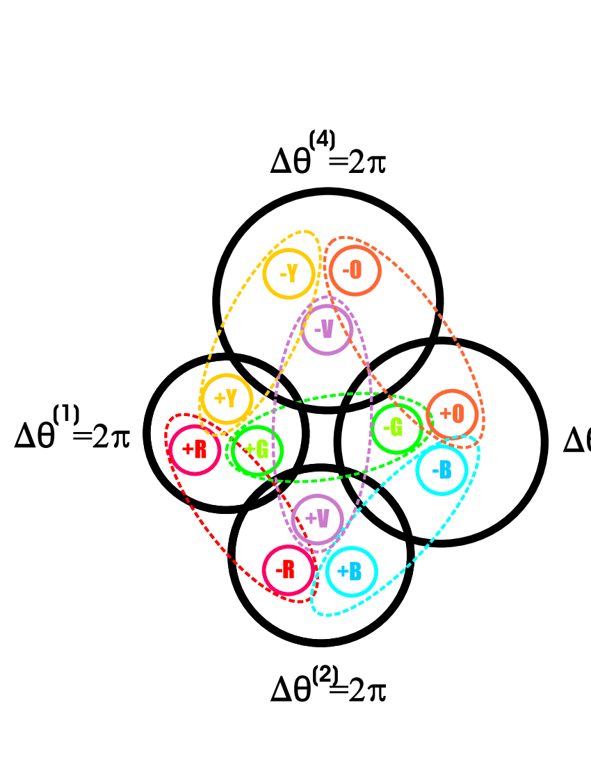
Figure 30: (Color online). A color charge representation for $N=4$ of the composite vortex lattice phase. This low-temperature phase, where the fluctuations of the composite vortex lines only involve small excursions of each of the constituent vortex lines away from the main composite object, may be viewed as a “6-color dielectric” phase. Moreover, for $N=4$, each type-$\alpha$ vortex in the $N=4$ case is a bound state of $3$ color charges. The dotted ellipses indicate which colors are involved in forming the dielectric phase.

Figure 31: (Color online). A color charge representation for $N=4$ of the first partial decomposition transition. In the color charge representation, this may be viewed as a $\rm{red}$-$\rm{green}$-$\rm{yellow}$ dielectric-metal transition, while the $\rm{violet}$-$\rm{blue}$-$\rm{orange}$ dielectric phase remains intact. As explained in the text, this partial 3-color metal-insulator transition involving fluctuating line charges, is in the 3D$xy$ universality class. The arrows indicate which three colors are involved in the metal-insulator transition. The dotted ellipses indicate which colors are involved in forming the remaining dielectric phase.

Figure 32: (Color online). A color charge representation for $N=4$ of the second partial decomposition transition. In the color charge representation, this may be viewed as a $\rm{violet}$-$\rm{blue}$ dielectric-metal transition, while the $\rm{orange}$ dielectric phase remains intact. As explained in the text, this partial 2-color metal-insulator transition involving fluctuating line charges, is in the 3D$xy$ universality class. The arrows indicate which two colors are involved in the metal-insulator transition. The dotted ellipse indicates which color is involved in forming the remaining dielectric phase.

Figure 33: (Color online). A color charge representation for $N=4$ of the third and complete decomposition transition. In the color charge representation, this may be viewed as an $\rm{orange}$ dielectric-metal transition, while the color-dielectric phase is completely destroyed. As explained in the text, this partial 1-color metal-insulator transition involving fluctuating line charges, is in the 3D$xy$ universality class. The arrow indicates which color is involved in the metal-insulator transition.

VIII.4 General $N$

In the general $N$-component case, the number of color charges that needs to be introduced to give an equivalent description as the above, may be counted as follows, starting from the third term in Eq. (4). Each combination $\theta^{(\alpha)}-\theta^{(\beta)}$ is given a color. We start with one phase, the one with the lowest bare stiffness say $\theta^{(1)}$, and introduce a non-trivial phase winding $\pm 2\pi$ in this phase. This excites $N-1$ neutral modes since $N-1$ gauge-invariant phase differences which involve $\theta^{(1)}$ can be formed. Introducing non-trivial phase-windings in the next phase $\theta^{(2)}$, the one with the next-to-lowest bare stiffness say, will also excite $N-1$ neutral modes, but only $N-2$ new neutral modes. Non-trivial phase-windings in the third phase $\theta^{(3)}$ will excite $N-3$ new neutral modes, and so on. The number of different colors $N_{\rm color}$ we will have to introduce for a theory with $N$ flavors of scalar fields is therefore given by $N_{\rm color}(N)=(N-1)+(N-2)+(N-3)+\dots+2+1=N(N-1)/2$, i.e.$N_{\rm color}(2)=1$, $N_{\rm color}(3)=3$, $N_{\rm color}(4)=6$, and $N_{\rm color}(5)=10$. A completely composite vortex, which we denote as an $N$-composite vortex, consists of $N$ constituent vortices originating in nontrivial phase windings in each of the individual phases $\theta^{(\alpha)},\alpha\in[1,\dots,N]$. Since a non-trivial phase winding in any phase $\theta^{(\eta)}$, $\eta\in[1,\dots,N]$, excites $N-1$ neutral modes $\theta^{(\eta)}-\theta^{(\alpha)}$, it is clear that a type-$\eta$ vortex may be viewed as a bound state of $N-1$ color charges. The particular combination of $N-1$ color charges, out of the total collection of $N(N-1)/2$ color charges, that will enter the $N-1$-body bound state in each vortex, will depend on $\eta$. The $N$-composite vortex is a color charge neutral object.

Small fluctuations in the $N$-composite vortex may therefore be viewed as a dielectric insulating phase of an $N(N-1)/2$-component dielectric. The first stage in the $N-1$ stage decomposition process of the $N$-composite vortex line, where a type-$1$ vortex tears itself off the $N$-composite vortex, is therefore a metal-insulator transition where $N-1$ color charges of the $N(N-1)/2$-colors dielectric system simultaneously undergo a metal insulator transition, in the 3D$xy$ universality class. The next stage, where a type-$2$ vortex tears itself off the remaining $N-1$-composite vortex in the background of a system of proliferated type-$1$ loops, is phase where $N-2$ color charges simultaneously undergo a metal insulator transition in the 3D$xy$ universality class by the same argument as used for the $N=3$ case, and so on. The complete decomposition of the $N$-composite vortex proceeds in $N-1$ steps of metal-insulator transitions for color charges, where step number $1\leq{\cal N}\leq N-1$ may be viewed as either a type-${\cal N}$ vortex tearing itself off an $N-{\cal N}-1$-composite vortex line, or equivalently a simultaneous metal-insulator transition for $N-{\cal N}$ new color charges that have not been involved in the previous ${\cal N}-1$ metal-insulator transitions. All the $N-1$ partial decomposition transitions, or metal-insulator transitions for color charges, are in the 3D$xy$ universality class.

We should emphasize that, as follows from Eq. (4) in the limit $N\to\infty$, the strength of each of the electric charges goes to zero. At the same time the number of colors of electric charges $N_{c}$ tends to infinity. From Eq. (4), it follows that even in the limit $N\to\infty$, the energy binding of a type-$\alpha$ vortex to a color charge neutral composite vortex is finite, even though the strength of each individual color charge tends to zero.

VIII.5 Graphical representation of phase disordering transitions in the $N=3$ model.

In Fig. 34, we illustrate graphically the various phase disordering transitions and partial symmetry restorations discussed in the previous section.

Figure 34: (Color online). A schematic plot of states in the $N=3$ system. The upper left panel shows the phases of the condensate order parameters that are involved. The upper right panel shows the state where all three phases $\theta^{(1)}$, $\theta^{(2)}$, and $\theta^{(3)}$ are ordered individually. This state is the low-temperature (ground) state and features one superconducting charged mode and two superfluid neutral modes. The middle left panel is a phase where $\theta^{(1)}$ is disordered, while $\theta^{(2)}$ and $\theta^{(3)}$ are ordered. Thus, this is a state which features one charged superconducting mode and one neutral superfluid mode. The middle right panel illustrates a state where all of the phases $\theta^{(1)}$, $\theta^{(2)}$, and $\theta^{(3)}$ are individually disordered. However, the differences $\theta^{(1)}-\theta^{(2)}$ and $\theta^{(2)}-\theta^{(3)}$ (and therefore also $\theta^{(1)}-\theta^{(3)}$) feature long-range order. This is therefore a state which is normal metallic, but nevertheless features two neutral superfluid modes. The bottom left panel illustrates a state where all of the phases $\theta^{(1)}$, $\theta^{(2)}$, and $\theta^{(3)}$ are individually disordered. Only the phase difference $\theta^{(2)}-\theta^{(3)}$ exhibits long-range order. This is a normal metallic state featuring one neutral superfluid mode. The bottom right panel illustrates a state where all of the phases $\theta^{(1)}$, $\theta^{(2)}$, and $\theta^{(3)}$ are individually disordered and where none of the phase differences $\theta^{(1)}-\theta^{(2)}$ and $\theta^{(2)}-\theta^{(3)}$ and $\theta^{(1)}-\theta^{(2)}$ feature long-range order. This is therefore a state which is normal metallic and normal fluid (no neutral superfluid modes). The states illustrated in the upper left, middle left, and lower right panel exist at zero as well as finite magnetic fields. The states illustrated in the middle right and lower left panels only exist at finite magnetic fields.

IX Applications

In this Section, we will briefly mention some possible applications of the results obtained in this paper. Emphasis will be on the case $N=2$, but some results for the cases $N=3$ and even $N=4$ may find applications in mixtures of superconducting condensates in the not too distant future.

IX.1 Applications of results for $N=2$

The results for $N=2$ are expected to apply to two-component superconductivity which could be achieved in metallic states of light atomsAshcroft1999 ; Neilnew , such as electronic and protonic condensates in liquid metallic hydrogen (LMH) under extreme pressure. Estimates exist for $T_{\rm c2}$ for such systems, $T_{\rm c2}\approx 160{\rm K}$ Ashcroft1999 . A rough estimate for $T_{\rm c1}$ follows from the mass ratio of the electronic and protonic condensate, $T_{\rm c1}\approx 0.1{\rm K}$. Hence, at $T_{\rm c1}$ one should observe an extra low-temperature 3D$xy$ specific heat anomaly, as well as an anomaly in the London penetration depth. An even more promising candidate is the the system $CH_{x}$ Neilnew where there are predictions of liquid metallic states at considerably lower pressures than those required to achieve LMH. In such multi-flavor superconductors it is the case $|\psi^{(1)}|\neq|\psi^{(2)}|$ which appears most naturally smiseth2004 .

Here, it is appropriate to remark briefly on the microscopic origins of superconductivity in the projected liquid metallic phase of hydrogen Ashcroft1999 ; Neilnew . The proton is four times lighter than a ${}^{4}He$ atom. It is well known that ${}^{4}He$ at normal conditions is a classic permanent liquid, because of high zero-point energy and weak ordering energies. Indeed zero-point energies of protons in a dense environment are also high, and at increasing compression there is a shift of electron density from intra-molecular regions to inter-molecular, and with it a progressive decline in the effective inter-proton attractions. Because of this there is also a decline of ordering energies from interactions relative to protonic zero-point energies. The existence of a melting point maximum as a function of pressure in hydrogen, as well as a range of densities where hydrogen may take up a fluid phase in its ground state was suggested in Ref. Ashcroft1999, . Another important circumstance is that en route hydrogen should undergo an insulator-metal transition and therefore the resulting phase should be the liquid metallic hydrogen, a translationally invariant two-component fermionic liquid. There is preliminary experimental evidence that a melting point maximum may indeed exist Datchi2000 and it has received recent powerful backing in ab initio calculations Bonev . Experimentally a 12.4 fold compression of hydrogen has already been achieved at around 320 ${\rm GPa}$ Datchi2000 ; Bonev . Estimates suggest that LMH should appear at 13.6 fold compression at pressure in the vicinity of 400 ${\rm GPa}$ Bonev , whereas hydrogen alloys may exhibit metallic behavior at significantly lower pressures Neilnew . A predicted key feature of LMH at low temperature is the coexistence of superconductivity of proton-proton and electron-electron Cooper pairs Ashcroft1999 .

The special point $|\psi^{(1)}|=|\psi^{(2)}|$ has a physical realization when Eq. (1) is viewed as an effective field theory of a quantum antiferromagnet with easy plane anisotropy, which facilitates a suppression of topological defects in the form of ”hedgehog”-configurations which appear in $O(3)$-symmetric models motrunich2004 ; sachdev2004 . (More generally, it may be viewed as a field theory of an $O(3)$ model where ”hedgehogs” are suppressed by some unspecified mechanism, not necessarily limited to easy-plane anisotropy).

We conclude this subsection on the $N=2$ case with a remark on how these results relate to multi-flavor electronic condensates. To describe this case, we need to include a Josephson coupling between the matter field species. The details of how to give a vortex representation of the $N$-flavor London model in the presence of inter-flavor Josephson coupling, is given in Appendix E. Had a Josephson coupling term between condensate species been introduced in the theory for $N\geq 2$, this would have have altered the dual theory in a completely non-perturbative way, and would tend to lock the phases of individual condensate fields to each other. (For a dual representation of this case, where the non-perturbative character of the Josephson coupling is brought out in a particularly clear way, see Appendix E). As a result, the transitions we describe here would collapse to one, namely the charged Higgs fixed point, which is in the inverted 3D$xy$ universality class.

IX.2 Applications of results for $N=3,4$

Mixtures of superconducting condensates in LMH can be extended to include also the hydrogen-isotopes deuterium and tritium thanksneil . Tritium is a $S=1/2$ fermion, so this may give rise to a superconducting condensate via forming spin-singlet Cooper pairs, just as in the protonic case. Hence, our results for $N=3$ could be applicable to to the mixtures of liquid metallic hydrogen-tritium at extremely high pressures. Another possibility is to include deuterium as a new component. Including deuterium as a new component in addition to hydrogen means that we have an $N=3$-component mixture of superconducting condensates consisting of electrons, protons, and deuterons (deuterium nuclei), all of which in principle can undergo a metal-superconductor transition. Compared to the situation for $N=2$, the situation is complicated by at least two circumstances. Firstly, deuterons are bosons, and secondly they have spin $S=1$. This means that the electrons and protons become superconducting via forming Cooper pairs, while the deuterons undergo a metal-superconducting transition via Bose-Einstein Condensation. Extending this to the case of having both tritium and deuterium in addition to hydrogen, might provide a realization of the case $N=4$.

X Summary

We have analyzed the $N$-flavor London superconductor model coupled to one gauge field with no Josephson coupling between the matter field components. The dual theory is an $N$-flavor GL theory coupled to $N$ dual gauge fields, where the sum of all dual gauge fields is massive at all couplings. There are $N-1$ charge-neutral superfluid modes and one charged superconducting mode in this model. We have given a prescription for how to identify the $N-1$ neutral modes for arbitrary $N$.

For $N=2$, a case which should apply to a superconducting state of liquid metallic hydrogen, as well as for the case $N=3$, we have performed large scale MC simulations computing i) critical exponents $\alpha$ and $\nu$, ii) gauge field and dual gauge field correlators, iii) the corresponding masses, and iv) critical couplings using FSS. For $N=2$ and $|\psi^{(1)}|\neq|\psi^{(2)}|$, we find one low-temperature critical point in the 3D$xy$ universality class at $T_{\rm c1}$, and one critical point in the inverted 3D$xy$ universality class at $T_{\rm c2}>T_{\rm c1}$. For $N=2$ with $|\psi^{(1)}|=|\psi^{(2)}|$ we find one critical point with non-3D$xy$ values of $\alpha$ and $\nu$ motrunich2004 . We propose these to be critical exponents in the universality class of a self-dual gauge theory. For $N=3$ and all $|\psi^{(\alpha)}|$ unequal, we find two fixed points in the 3D$xy$ universality class at $T_{\rm c1}$ and $T_{\rm c2}$, and one fixed point in the inverted 3D$xy$ universality class at $T_{\rm c3}(>T_{\rm c2}>T_{\rm c1})$. All critical points therefore exhibit 3D$xy$ values of $\alpha$ and $\nu$ when all bare phase stiffnesses $|\psi^{(\alpha)}|$ are different. In the case $N=3$ with $|\psi^{(1)}|=|\psi^{(2)}|<|\psi^{(3)}|$ we find two critical points. The critical point at $T_{\rm c1}<T_{\rm c2}$ is found to be in the 3D$xy$ universality class, and the critical point at $T_{\rm c2}$ is in the inverted 3D$xy$ universality class. For the case $N=3$ with equal phase stiffnesses we find one critical point which is non-3D$xy$ .

In this context, we have also noted that collapsing two neutral critical points in the 3D$xy$ universality class leads to a single critical point also in the 3D$xy$ universality class. This follows from an argument implying that collapsing any number of neutral critical points in the 3D$xy$ universality class leads to a single critical point also in the 3D$xy$ universality class. On the other hand, it appears that collapsing $N-1$ neutral critical points in the 3D$xy$ universality class and one charged fixed point in the inverted 3D$xy$ universality class leads to a single critical point in a universality class (which in principle could depend on $N$) which is not that of the 3D$xy$ or inverted 3D$xy$ type. For $N=2$, we may define the universality class as that of a 3D self-dual $U(1)\times U(1)$ gauge theory, while it is less clear what it is for other $N\geq 3$. The numerical values we have obtained for the critical exponents $\alpha$ and $\nu$ the two cases i) $N=2$, $|\psi^{(1)}|=|\psi^{(2)}|$ and ii) $N=3$, $|\psi^{(1)}|=|\psi^{(2)}|=|\psi^{(3)}|$ are remarkably similar, indicating that the values of the critical exponents are at most weakly dependent on $N$.

In an external magnetic field at low temperature, the ground state of the system is an Abrikosov vortex lattice of composite vortices. However the effect of thermal fluctuations alters the physics significantly. We discuss in detail that in the low-field regime and when the bare stiffnesses of the condensates all differ, we find that a 3D$xy$ vortex sub-lattice melting transition takes place. Upon thermal decomposition of field induced composite vortex lines, the constituent vortices originating in the condensates with lowest bare stiffness disorder, while the ones originating in the stiffer condensates remain arranged in an Abrikosov vortex lattice. When such a transition occurs, an $N=2$ system looses superfluid properties, but remains superconducting. In contrast at high magnetic fields, the neutral mode disappears via the melting transition of the lattice of composite vortices. This is a transition from the superconducting state to a non-superconducting metallic superfluid state BSA . Inside this novel metallic superfluid phase, at a temperature much lower than the zero-field metal-superconductor transition, we find a superfluid-normal fluid 3D$xy$ phase transition associated with a neutral mode-driven proliferation of vortex loops nucleating on field-induced vortex lines. These various transitions should in principle be detectable in flux-noise experiments. We extend the discussion for $N>2$, where we find phase transitions associated with partial decomposition of composite vortices, yielding several unusual states of partial symmetry breakdown. The universality class and partial symmetry breakdowns are identified by mapping the system to an ensemble of electrically charged strings where for the $N$-component system there are $N(N-1)/2$ replicas of electric charges of different color.

The sublattice melting and partial decomposition transitions are of purely topological origin. It involves what can be viewed as vortices and anti-vortices (positively and negatively charged objects). The existence of positively and negatively charged objects implies that the physics conceptually in some sense is similar to what occurs in a Kosterlitz-Thouless (KT) transition in two dimensions. In spite of being a decomposition of positively and negatively charged composite objects, such a transition can be mapped onto a proliferation of vortex loops in a vacuum, i.e a phase transition in the 3D$xy$ universality class. Another principal difference between this type of phase transition compared to the KT transition, is that in the 2D KT transition, vortices and anti-vortices (positively and negatively charged objects) are thermally generated. This can not happen in three dimensions since any vortex line in 3D has an infinite energy in an infinite sample. In the 3D transition which we consider, the neutral bound states of the charged objects are introduced by an external magnetic field. Thus we deal with a novel type of transition which in a very unusual form involves concepts both from two- and three- dimensional physics.

Appendix A Identifying charged and neutral modes

Here, we illustrate in detail the separation of variables in $N$-component London model and the extraction of the composite charged and neutral modes in the London limit. The general procedure beyond the London limit for the case $N=2$ can be found in egor2002 . The general $N$-component Ginzburg-Landau model is given by the action

$$S=\sum_{\mathbf{r}}\left\{\sum_{\alpha=1}^{N}\frac{1}{2}{|(\nabla-{\rm i}e\mathbf{A})\psi^{(\alpha)}|^{2}}+V(\{\psi^{(\alpha)}\})+\frac{1}{2}(\nabla\times\mathbf{A})^{2}\right\}.$$ (60)

Here, the masses $M^{(\alpha)}$ have been absorbed in the amplitudes $|\psi^{(\alpha)}|$ for notational simplicity. Let us rewrite the first term in Eq. (60) as follows

$$\sum_{\alpha=1}^{N}\frac{1}{2}{|(\nabla-{\rm i}e\mathbf{A})\psi^{(\alpha)}|^{2}} = \sum_{\alpha=1}^{N}\frac{1}{2}|\psi^{(\alpha)}|^{2}(\nabla\theta^{(\alpha)})^{2}-e\mathbf{A}\cdot(\nabla\theta^{(\alpha)})|\psi^{(\alpha)}|^{2}+\frac{1}{2}e^{2}\mathbf{A}^{2}|\psi^{(\alpha)}|^{2}.$$ (61)

The idea now is to first extract the charged mode of the system, and then identify the remaining terms as the neutral modes. The charged modes is the (only) linear combination of phase gradients $\nabla\theta^{(\alpha)}$ that couples to the gauge field $\mathbf{A}$. We first introduce the quantity

$$\mathbf{\Theta}\equiv\sum_{\alpha=1}^{N}|\psi^{(\alpha)}|^{2}\nabla\theta^{(\alpha)}.$$ (62)

Using this, we form the combination

$$\left(\sum_{\alpha=1}^{N}|\psi^{(\alpha)}|^{2}\left[\nabla\theta^{(\alpha)}-e\mathbf{A}\right]\right)^{2}=(\mathbf{\Theta}-e\Psi^{2}\mathbf{A})^{2},$$ (63)

where $\Psi^{2}$ is defined in Eq. (5). One can check that this combination is gauge-invariant. By adding and subtracting ${\mathbf{\Theta}}^{2}/{2\Psi^{2}}$, we now express Eq. (61) as follows

$$\sum_{\alpha=1}^{N}\frac{1}{2}|\psi^{(\alpha)}|^{2}(\nabla\theta^{(\alpha)})^{2}-e\mathbf{A}\cdot(\nabla\theta^{(\alpha)})|\psi^{(\alpha)}|^{2}+\frac{1}{2}e^{2}\mathbf{A}^{2}|\psi^{(\alpha)}|^{2}=$$

$$\frac{1}{2}\left[\sum_{\alpha=1}^{N}|\psi^{(\alpha)}|^{2}(\nabla\theta^{(\alpha)})^{2}-\frac{\mathbf{\Theta}^{2}}{\Psi^{2}}\right]+\frac{1}{2\Psi^{2}}(\mathbf{\Theta}-e\Psi^{2}\mathbf{A})^{2}.$$ (64)

The last term is identified as the charged mode. The first term on the right hand side of Eq. (64) can be rewritten as follows

$$\frac{1}{2}\left[\sum_{\alpha=1}^{N}|\psi^{(\alpha)}|^{2}(\nabla\theta^{(\alpha)})^{2}-\frac{\mathbf{\Theta}^{2}}{\Psi^{2}}\right] = \frac{1}{2\Psi^{2}}\left[\sum_{\alpha,\beta=1}^{N}|\psi^{(\alpha)}|^{2}|\psi^{(\beta)}|^{2}\nabla\theta^{(\alpha)}(\nabla\theta^{(\alpha)}-\nabla\theta^{(\beta)})\right]$$ (65)

$$= \frac{1}{4\Psi^{2}}\left[\sum_{\alpha,\beta=1}^{N}|\psi^{(\alpha)}|^{2}|\psi^{(\beta)}|^{2}(\nabla\theta^{(\alpha)}-\nabla\theta^{(\beta)})^{2}\right].$$

Therefore, the action may be expressed as

$$S=\sum_{\mathbf{r}}\left\{\left(\frac{1}{2\Psi^{2}}\sum_{\alpha=1}^{N}|\psi^{(\alpha)}|^{2}\nabla\theta^{(\alpha)}-e\Psi^{2}\mathbf{A}\right)^{2}+\frac{1}{2}(\nabla\times\mathbf{A})^{2}+\frac{1}{4\Psi^{2}}\left[\sum_{\alpha,\beta=1}^{N}|\psi^{(\alpha)}|^{2}|\psi^{(\beta)}|^{2}\left(\nabla(\theta^{(\alpha)}-\theta^{(\beta)})\right)^{2}\right]\right\},$$ (66)

which is now a sum of one charged mode and $N-1$ neutral modes. The last term in Eq. (66) is a sum consisting of $N(N-1)/2$ terms, involving all the color charges $(\theta^{(\alpha)}-\theta^{(\beta)})$ (see Section VIII) which are needed to account for all the possible ways neutral modes can be excited in the system as a consequence of multiple connectedness of physical space in the presence of vortices. Note how this term vanishes when $N=1$.

Appendix B Derivation of Eqs. (11) and (12)

Starting from the model in the Villain approximation Eq. (7) we linearize the kinetic energy terms by introducing $N$ auxiliary fields $\mathbf{v}^{(\alpha)}$ where $\alpha\in 1,\dots,N$ with a partition function

$$\begin{split}Z=&\int_{-\infty}^{\infty}\mathcal{D}\mathbf{A}\prod_{\gamma=1}^{N}\int_{-\pi}^{\pi}\mathcal{D}\theta^{(\gamma)}\int_{-\infty}^{\infty}\mathcal{D}\mathbf{v}^{(\gamma)}\sum_{\ \mathbf{n}^{(\gamma)}}\exp(-S),\\ S=&\sum_{\mathbf{r}}\left(\sum_{\alpha=1}^{N}\frac{1}{2\beta|\psi^{(\alpha)}|^{2}}(\mathbf{v}^{(\alpha)})^{2}+\sum_{\alpha=1}^{N}{\rm i}(\Delta\theta^{(\alpha)}-e\mathbf{A}+2\pi\mathbf{n}^{(\alpha)})\cdot\mathbf{v}^{(\alpha)}+\frac{\beta}{2}(\Delta\times\mathbf{A})^{2}\right),\end{split}$$ (67)

where $|\psi^{(\alpha)}|^{2}=|\Psi^{(\alpha)}_{0}|^{2}/M^{(\alpha)}$. The Poisson summation formula reads

$$\sum_{n=-\infty}^{\infty}{\rm e}^{2\pi inB}=\sum_{m=-\infty}^{\infty}\delta(m-B).$$ (68)

Here, $n,m\in\mathbb{Z}$ and $B\in\mathbb{R}$. We apply Eq. (68) to Eq. (67) and integrate out the integer fields $\mathbf{n}^{(\alpha)}$ so that the fields $\mathbf{v}^{(\alpha)}$ take only integer values which we denote $\mathbf{\hat{v}}^{(\alpha)}$. After a partial summation of $\sum_{\mathbf{r}}\sum_{\alpha=1}^{N}{\rm i}\Delta\theta^{(\alpha)}\cdot\mathbf{\hat{v}}^{(\alpha)}=-\sum_{\mathbf{r}}\sum_{\alpha=1}^{N}{\rm i}\theta^{(\alpha)}\Delta\cdot\mathbf{\hat{v}}^{(\alpha)}$, where the surface terms are omitted, we may integrate out the phase fields $\theta^{(\alpha)}$. This integration produces the local constraints

$$\Delta\cdot\mathbf{\hat{v}}^{(\alpha)}=0.$$ (69)

To fulfill this constraint we let $\mathbf{\hat{v}}^{(\alpha)}=\Delta\times\mathbf{\hat{h}}^{(\alpha)}$ where $\mathbf{\hat{h}}^{(\alpha)}$ is an integer-valued vector field. At this point the theory reads

$$\begin{split}Z=&\int_{-\infty}^{\infty}\mathcal{D}\mathbf{A}\prod_{\gamma=1}^{N}\sum_{\ \mathbf{\hat{h}}^{(\gamma)}}\exp(-S),\\ S=&\sum_{\mathbf{r}}\left[\sum_{\alpha=1}^{N}\frac{1}{2\beta|\psi^{(\alpha)}|^{2}}(\Delta\times\mathbf{\hat{h}}^{(\alpha)})^{2}-{\rm i}e\mathbf{A}\cdot\left(\sum_{\alpha=1}^{N}\Delta\times\mathbf{\hat{h}}^{(\alpha)}\right)+\frac{\beta}{2}(\Delta\times\mathbf{A})^{2}\right].\end{split}$$ (70)

Again, we apply the Poisson summation formula Eq. (68) and the integer fields $\mathbf{\hat{h}}^{(\alpha)}$ are replaced by continuous dual gauge fields $\mathbf{h}^{(\alpha)}$ at the cost of introducing the term $2\pi{\rm i}\sum_{\alpha}\mathbf{h}^{(\alpha)}\cdot\mathbf{m}^{(\alpha)}$ in the action and $\mathbf{m}^{(\alpha)}$ are integer vortex fields. Then the partition function reads

$$\begin{split}Z=&\int_{-\infty}^{\infty}\mathcal{D}\mathbf{A}\prod_{\gamma=1}^{N}\int_{-\infty}^{\infty}\mathcal{D}\mathbf{h}^{(\gamma)}\sum_{\ \mathbf{m}^{(\gamma)}}\delta_{\Delta\cdot\mathbf{m}^{(\gamma)},0}\exp(-S),\\ S=&\sum_{\mathbf{r}}\left[\sum_{\alpha=1}^{N}\frac{1}{2\beta|\psi^{(\alpha)}|^{2}}(\Delta\times\mathbf{h}^{(\alpha)})^{2}-{\rm i}e\mathbf{A}\cdot\left(\sum_{\alpha=1}^{N}\Delta\times\mathbf{h}^{(\alpha)}\right)+2\pi{\rm i}\sum_{\alpha=1}^{N}\mathbf{h}^{(\alpha)}\cdot\mathbf{m}^{(\alpha)}+\frac{\beta}{2}(\Delta\times\mathbf{A})^{2}\right],\end{split}$$ (71)

where $\delta_{n,m}$ is the Kronecker delta. The gauge symmetry of the integer valued fields $\mathbf{\hat{h}}^{(\alpha)}$ in Eq. (70) must be preserved through this transformation. Hence, the action Eq. (71) must be invariant under the gauge transformation $\mathbf{h}^{(\alpha)}\to\mathbf{h}^{(\alpha)}+\Delta\chi$. The transformation produces the term $\sum_{\mathbf{r}}\sum_{\alpha}2\pi{\rm i}\Delta\chi\cdot\mathbf{m}^{(\alpha)}$ which must be zero to preserve gauge symmetry. A partial summation therefore produces the constraint $\Delta\cdot\mathbf{m}^{(\alpha)}=0$ on each flavor of the vortex fields. At this point it is useful to write the theory in the Fourier representation and the action becomes

$$\begin{split}S=&\sum_{\mathbf{q}}\left\{\sum_{\alpha=1}^{N}\frac{1}{2\beta|\psi^{(\alpha)}|^{2}}(\mathbf{Q}_{\mathbf{q}}\times\mathbf{h}_{\mathbf{q}}^{(\alpha)})\cdot(\mathbf{Q}_{-\mathbf{q}}\times\mathbf{h}_{-\mathbf{q}}^{(\alpha)})+\pi{\rm i}\sum_{\alpha=1}^{N}\left[\mathbf{h}^{(\alpha)}_{\mathbf{q}}\cdot\mathbf{m}^{(\alpha)}_{-\mathbf{q}}+\mathbf{h}^{(\alpha)}_{-\mathbf{q}}\cdot\mathbf{m}^{(\alpha)}_{\mathbf{q}}\right]\right.\\ &\left.-\frac{{\rm i}e}{2}\left[\mathbf{A_{\mathbf{q}}}\cdot\left(\sum_{\alpha=1}^{N}\mathbf{Q}_{-\mathbf{q}}\times\mathbf{h}^{(\alpha)}_{-\mathbf{q}}\right)+\mathbf{A_{-\mathbf{q}}}\cdot\left(\sum_{\alpha=1}^{N}\mathbf{Q}_{\mathbf{q}}\times\mathbf{h}^{(\alpha)}_{\mathbf{q}}\right)\right]+\frac{\beta}{2}(\mathbf{Q}_{\mathbf{q}}\times\mathbf{A}_{\mathbf{q}})\cdot(\mathbf{Q}_{-\mathbf{q}}\times\mathbf{A}_{-\mathbf{q}})\right\},\end{split}$$ (72)

where $\mathbf{Q}_{\mathbf{q}}$ is the Fourier representation of the lattice difference operator $\Delta$. We choose the gauge $\Delta\cdot\mathbf{A}=0$ and $\Delta\cdot\mathbf{h}^{(\alpha)}=0$ which in the Fourier representation is $\mathbf{Q}_{\mathbf{q}}\cdot\mathbf{A}_{\mathbf{q}}=0$ and $\mathbf{Q}_{\mathbf{q}}\cdot\mathbf{h}^{(\alpha)}_{\mathbf{q}}=0$. We complete the squares in $\mathbf{A}_{\mathbf{q}}$ and get the action

$$\begin{split}S=&\sum_{\mathbf{q}}\left\{\sum_{\alpha=1}^{N}\frac{1}{2\beta|\psi^{(\alpha)}|^{2}}(\mathbf{Q}_{\mathbf{q}}\cdot\mathbf{Q}_{-\mathbf{q}})(\mathbf{h}_{\mathbf{q}}^{(\alpha)}\cdot\mathbf{h}_{-\mathbf{q}}^{(\alpha)})+\pi{\rm i}\sum_{\alpha=1}^{N}\left[\mathbf{h}^{(\alpha)}_{\mathbf{q}}\cdot\mathbf{m}^{(\alpha)}_{-\mathbf{q}}+\mathbf{h}^{(\alpha)}_{-\mathbf{q}}\cdot\mathbf{m}^{(\alpha)}_{\mathbf{q}}\right]\right.\\ &+\left.\left[\mathbf{A}_{\mathbf{q}}-\frac{{\rm i}e}{2}\left(\sum_{\alpha=1}^{N}\mathbf{Q}_{\mathbf{q}}\times\mathbf{h}^{(\alpha)}_{\mathbf{q}}\right)D_{\mathbf{q}}^{-1}\right]D_{\mathbf{q}}\left[\mathbf{A}_{-\mathbf{q}}-\frac{{\rm i}e}{2}\left(\sum_{\alpha=1}^{N}\mathbf{Q}_{-\mathbf{q}}\times\mathbf{h}^{(\alpha)}_{-\mathbf{q}}\right)D_{\mathbf{q}}^{-1}\right]\right.\\ &+\left.\frac{e^{2}}{4}\left(\sum_{\alpha=1}^{N}\mathbf{Q}_{\mathbf{q}}\times\mathbf{h}^{(\alpha)}_{\mathbf{q}}\right)D_{\mathbf{q}}^{-1}\left(\sum_{\alpha=1}^{N}\mathbf{Q}_{-\mathbf{q}}\times\mathbf{h}^{(\alpha)}_{-\mathbf{q}}\right)\right\},\end{split}$$ (73)

where $D_{\mathbf{q}}=\beta\mathbf{Q}_{\mathbf{q}}\cdot\mathbf{Q}_{-\mathbf{q}}/2$. After performing the gaussian integral in $\mathbf{A}_{\mathbf{q}}$, the action reads

$$\begin{split}S=&\sum_{\mathbf{q}}\left\{\sum_{\alpha=1}^{N}\frac{1}{2\beta|\psi^{(\alpha)}|^{2}}(\mathbf{Q}_{\mathbf{q}}\cdot\mathbf{Q}_{-\mathbf{q}})(\mathbf{h}_{\mathbf{q}}^{(\alpha)}\cdot\mathbf{h}_{-\mathbf{q}}^{(\alpha)})+\pi{\rm i}\sum_{\alpha=1}^{N}\left[\mathbf{h}^{(\alpha)}_{\mathbf{q}}\cdot\mathbf{m}^{(\alpha)}_{-\mathbf{q}}+\mathbf{h}^{(\alpha)}_{-\mathbf{q}}\cdot\mathbf{m}^{(\alpha)}_{\mathbf{q}}\right]\right.\\ &+\left.\frac{e^{2}}{2\beta}\left(\sum_{\alpha=1}^{N}\mathbf{h}^{(\alpha)}_{\mathbf{q}}\right)\cdot\left(\sum_{\alpha=1}^{N}\mathbf{h}^{(\alpha)}_{-\mathbf{q}}\right)\right\}.\end{split}$$ (74)

At this point it is useful to introduce matrices and vectors in flavor indices. We write the action as

$$S=\sum_{\mathbf{q}}\left[H^{\rm T}_{\mathbf{q}}G_{\mathbf{q}}H_{-\mathbf{q}}+{\rm i}\pi M^{\rm T}_{\mathbf{q}}H_{-\mathbf{q}}+{\rm i}\pi H^{\rm T}_{\mathbf{q}}M_{-\mathbf{q}}\right],$$ (75)

where $H^{\rm T}_{\mathbf{q}}=(\mathbf{h}^{(1)}_{\mathbf{q}},\mathbf{h}^{(2)}_{\mathbf{q}},\dots,\mathbf{h}^{(N)}_{\mathbf{q}})$ and $M^{\rm T}_{\mathbf{q}}=(\mathbf{m}^{(1)}_{\mathbf{q}},\mathbf{m}^{(2)}_{\mathbf{q}},\dots,\mathbf{m}^{(N)}_{\mathbf{q}})$ are vectors in flavor indices, and the matrix $G_{\mathbf{q}}$ is given by

$$G_{\mathbf{q}}=\left(\begin{array}[]{ccccc}\frac{|\mathbf{Q}_{\mathbf{q}}|^{2}}{2\beta|\psi^{(1)}|^{2}}+\frac{e^{2}}{2\beta}&\frac{e^{2}}{2\beta}&\cdots&\frac{e^{2}}{2\beta}&\frac{e^{2}}{2\beta}\\ \frac{e^{2}}{2\beta}&\frac{|\mathbf{Q}_{\mathbf{q}}|^{2}}{2\beta|\psi^{(2)}|^{2}}+\frac{e^{2}}{2\beta}&\cdots&\frac{e^{2}}{2\beta}&\frac{e^{2}}{2\beta}\\ \vdots&\ddots&\ddots&\ddots&\vdots\\ \frac{e^{2}}{2\beta}&\frac{e^{2}}{2\beta}&\cdots&\frac{|\mathbf{Q}_{\mathbf{q}}|^{2}}{2\beta|\psi^{(N-1)}|^{2}}+\frac{e^{2}}{2\beta}&\frac{e^{2}}{2\beta}\\ \frac{e^{2}}{2\beta}&\frac{e^{2}}{2\beta}&\cdots&\frac{e^{2}}{2\beta}&\frac{|\mathbf{Q}_{\mathbf{q}}|^{2}}{2\beta|\psi^{(N)}|^{2}}+\frac{e^{2}}{2\beta}\end{array}\right),$$ (76)

where $|\mathbf{Q}_{\mathbf{q}}|^{2}=\mathbf{Q}_{\mathbf{q}}\cdot\mathbf{Q}_{-\mathbf{q}}$. In flavor indices $\eta,\lambda$ we write the matrix as $G_{\mathbf{q}}^{(\eta,\lambda)}=d^{(\eta)}\delta_{\eta,\lambda}+c$, where $d^{(\eta)}=\frac{|\mathbf{Q}_{\mathbf{q}}|^{2}}{2\beta|\psi^{(\eta)}|^{2}}$ and $c=\frac{e^{2}}{2\beta}$. We complete the square and obtain the expression

$$S=\sum_{\mathbf{q}}\left[(H^{\rm T}_{\mathbf{q}}+{\rm i}\pi M^{\rm T}_{\mathbf{q}}G_{\mathbf{q}}^{-1})G_{\mathbf{q}}(H_{-\mathbf{q}}+{\rm i}\pi M_{-\mathbf{q}}G_{\mathbf{q}}^{-1})+\pi^{2}M^{\rm T}_{\mathbf{q}}G_{\mathbf{q}}^{-1}M_{-\mathbf{q}}\right],$$ (77)

where $G_{\mathbf{q}}^{-1}$ is the solution of $G_{\mathbf{q}}G_{\mathbf{q}}^{-1}=I$ and $I$ is the $N\times N$ unit matrix. Gaussian integration of $H_{\mathbf{q}}$ yields an action expressed in vortex variables of different flavors

$$S=\sum_{\mathbf{q}}\pi^{2}M^{\rm T}_{\mathbf{q}}G_{\mathbf{q}}^{-1}M_{-\mathbf{q}}.$$ (78)

The matrix $G_{\mathbf{q}}^{-1}$ is found to have the following diagonal elements

$$(G_{\mathbf{q}}^{-1})^{(\eta,\eta)}=\frac{\prod_{\alpha\neq\eta}d^{(\alpha)}+c\sum_{\alpha\neq\eta}\prod_{\gamma\neq\eta,\alpha}d^{(\gamma)}}{\prod_{\alpha=1}^{N}d^{(\alpha)}+c\sum_{\alpha=1}^{N}\prod_{\gamma\neq\alpha}d^{(\gamma)}},$$ (79)

and

$$(G_{\mathbf{q}}^{-1})^{(\eta,\lambda)}=-\frac{c\prod_{\alpha\neq\eta,\lambda}d^{(\alpha)}}{\prod_{\alpha=1}^{N}d^{(\alpha)}+c\sum_{\alpha=1}^{N}\prod_{\gamma\neq\alpha}d^{(\gamma)}},$$ (80)

as off-diagonal elements ($\eta\neq\lambda$), where $\prod_{\alpha=\varnothing}d^{(\alpha)}\equiv 1$. By dividing the numerator and denominator by $\prod_{\alpha=1}^{N}d^{(\alpha)}$, we obtain the diagonal elements

$$(G_{\mathbf{q}}^{-1})^{(\eta,\eta)}=\frac{\frac{1}{d^{(\eta)}}+\sum_{\alpha\neq\eta}\frac{c}{d^{(\eta)}d^{(\alpha)}}}{1+\sum_{\alpha=1}^{N}\frac{c}{d^{(\alpha)}}},$$ (81)

and the off-diagonal elements

$$(G_{\mathbf{q}}^{-1})^{(\eta,\lambda)}=-\frac{\frac{c}{d^{(\eta)}d^{(\lambda)}}}{1+\sum_{\alpha=1}^{N}\frac{c}{d^{(\alpha)}}},$$ (82)

where $\eta\neq\lambda$. In total, the matrix $(G_{\mathbf{q}}^{-1})^{(\eta,\lambda)}$ reads

$$(G_{\mathbf{q}}^{-1})^{(\eta,\lambda)}=\frac{(\frac{1}{d^{(\eta)}}+\sum_{\alpha=1}^{N}\frac{c}{d^{(\eta)}d^{(\alpha)}})\delta_{\eta,\lambda}-\frac{c}{d^{(\eta)}d^{(\lambda)}}}{1+\sum_{\alpha=1}^{N}\frac{c}{d^{(\alpha)}}}.$$ (83)

Inserting the expressions for $d^{(\eta)}$ and $c$ and multiplying by $|\mathbf{Q}_{\mathbf{q}}|^{4}$ in the denominator and numerator, we obtain

$$(G_{\mathbf{q}}^{-1})^{(\eta,\lambda)}=2\beta\frac{(|\psi^{(\eta)}|^{2}|\mathbf{Q}_{\mathbf{q}}|^{2}+e^{2}|\psi^{(\eta)}|^{2}\sum_{\alpha=1}^{N}|\psi^{(\alpha)}|^{2})\delta_{\eta,\lambda}-e^{2}|\psi^{(\eta)}|^{2}|\psi^{(\lambda)}|^{2}}{|\mathbf{Q}_{\mathbf{q}}|^{2}(|\mathbf{Q}_{\mathbf{q}}|^{2}+e^{2}\sum_{\alpha=1}^{N}|\psi^{(\alpha)}|^{2})}.$$ (84)

We introduce $\Psi^{2}=\sum_{\alpha=1}^{N}|\psi^{(\alpha)}|^{2}$ and split the expression by partial fractioning and obtain the matrix

$$(G_{\mathbf{q}}^{-1})^{(\eta,\lambda)}=\frac{2\beta|\psi^{(\eta)}|^{2}}{\Psi^{2}}\left[\frac{\Psi^{2}\delta_{\eta,\lambda}-|\psi^{(\lambda)}|^{2}}{|\mathbf{Q}_{\mathbf{q}}|^{2}}+\frac{|\psi^{(\lambda)}|^{2}}{|\mathbf{Q}_{\mathbf{q}}|^{2}+e^{2}\Psi^{2}}\right].$$ (85)

This is the vortex interaction matrix given in Eq. (12). Inserting this into Eq. (78), the partition function of the system is

$$\begin{split}Z=&\prod_{\alpha}\sum_{\mathbf{m}^{(\alpha)}}\delta_{\Delta\cdot\mathbf{m}^{(\alpha)},0}\exp(-S_{\rm V}),\\ S_{\rm V}=&\sum_{\mathbf{q}}\sum_{\eta,\lambda=1}^{N}\frac{2\pi^{2}\beta}{\Psi^{2}}\mathbf{m}^{(\eta)}_{\mathbf{q}}\cdot\mathbf{m}^{(\lambda)}_{-\mathbf{q}}|\psi^{(\eta)}|^{2}\left[\frac{\Psi^{2}\delta_{\eta,\lambda}-|\psi^{(\lambda)}|^{2}}{|\mathbf{Q}_{\mathbf{q}}|^{2}}+\frac{|\psi^{(\lambda)}|^{2}}{|\mathbf{Q}_{\mathbf{q}}|^{2}+e^{2}\Psi^{2}}\right],\end{split}$$ (86)

which gives the action in the partition function in Eq. (11). The above vortex action may be written in terms of charged and neutral vortex modes in a manner analogous to that of Eq. (66), as follows

$$\begin{split}\frac{S_{\rm V}}{2\pi^{2}\beta/\Psi^{2}}=&\sum_{\mathbf{q}}\left\{\frac{(\sum_{\alpha}|\psi^{(\alpha)}|^{2}\mathbf{m}^{(\alpha)}_{\mathbf{q}})\cdot(\sum_{\beta}|\psi^{(\beta)}|^{2}\mathbf{m}^{(\beta)}_{-\mathbf{q}})}{|\mathbf{Q}_{\mathbf{q}}|^{2}+m_{0}^{2}}+\sum_{\alpha,\beta}\frac{|\psi^{(\alpha)}|^{2}|\psi^{(\beta)}|^{2}(\mathbf{m}^{(\alpha)}_{\mathbf{q}}-\mathbf{m}^{(\beta)}_{\mathbf{q}})\cdot(\mathbf{m}^{(\alpha)}_{-\mathbf{q}}-\mathbf{m}^{(\beta)}_{-\mathbf{q}})}{2|\mathbf{Q}_{\mathbf{q}}|^{2}}\right\}.\end{split}$$ (87)

Here, $m_{0}^{2}=e^{2}\Psi^{2}$. While the first, screened, term in general is present for all $N\geq 1$, it is clear from the above formulation that the second, unscreened, term is only present provided $N\geq 2$. The factor $2$ in the denominator in the unscreened terms is essential in order for the interaction terms between different vortex species to cancel out when $m_{0}^{2}=0$.

Appendix C Gauge field correlator

Introducing Fourier-transformed variables in Eq. (10), prior to integrating out the gauge field $\mathbf{A}$, and adding source terms in the form of electric currents $\mathbf{J}$ coupling linearly to $\mathbf{A}$, we obtain the action (note that for convenience, we have redefined the $\mathbf{A}$-field in this Appendix by a factor $\sqrt{\beta}$ as follows: $\mathbf{A}\to\tilde{\mathbf{A}}=\sqrt{\beta}\mathbf{A}$, and then renaming $\tilde{\mathbf{A}}\to\mathbf{A}$. Thus, here we also redefine the charge as follows: $e\to\tilde{e}=e/\sqrt{\beta}$ which we then rename $\tilde{e}\to e$. In the end result we reinstate the original definitions. We thus have the action Eq. (10) on the form

$$S_{J} = \sum_{\mathbf{q}}\left[\frac{|\mathbf{Q}_{\mathbf{q}}|^{2}}{2\beta|\psi^{(\alpha)}|^{2}}\mathbf{h}^{(\alpha)}_{\mathbf{q}}\cdot\mathbf{h}^{(\alpha)}_{-\mathbf{q}}+\pi{\rm i}\left[\mathbf{m}^{(\alpha)}_{\mathbf{q}}\cdot\mathbf{h}^{(\alpha)}_{-\mathbf{q}}+\mathbf{m}^{(\alpha)}_{-\mathbf{q}}\cdot\mathbf{h}^{(\alpha)}_{\mathbf{q}}\right]-\frac{{\rm i}e}{2}\left[\mathbf{A}_{\mathbf{q}}\cdot(\mathbf{Q}_{-\mathbf{q}}\times\mathbf{h}^{(\alpha)}_{-\mathbf{q}})+(\mathbf{Q}_{\mathbf{q}}\times\mathbf{h}^{(\alpha)}_{\mathbf{q}})\cdot\mathbf{A}_{-\mathbf{q}}\right]\right.$$ (88)

$$+ \left.\frac{1}{2}\left[\mathbf{J}_{\mathbf{q}}\cdot\mathbf{A}_{-\mathbf{q}}+\mathbf{J}_{-\mathbf{q}}\cdot\mathbf{A}_{\mathbf{q}}\right]+\frac{|\mathbf{Q}_{\mathbf{q}}|^{2}}{2}\mathbf{A}_{\mathbf{q}}\cdot\mathbf{A}_{-\mathbf{q}}\right].$$

Summations over indices $(\alpha,\beta)\in[1,\dots,N]$ is understood. Integrating out the gauge fields $\mathbf{A}_{\mathbf{q}}$, we get the action on the following form

$$\tilde{S}_{J} = \sum_{\mathbf{q}}\sum_{\alpha=1}^{N}\left[\frac{|\mathbf{Q}_{\mathbf{q}}|^{2}}{2\beta|\psi^{(\alpha)}|^{2}}\mathbf{h}^{(\alpha)}_{\mathbf{q}}\cdot\mathbf{h}^{(\alpha)}_{-\mathbf{q}}+\pi{\rm i}\left[\mathbf{m}^{(\alpha)}_{\mathbf{q}}\cdot\mathbf{h}^{(\alpha)}_{-\mathbf{q}}+\mathbf{m}^{(\alpha)}_{-\mathbf{q}}\cdot\mathbf{h}^{(\alpha)}_{\mathbf{q}}\right]-\frac{\mathbf{D}_{\mathbf{q}}\cdot\mathbf{D}_{-\mathbf{q}}}{2|\mathbf{Q}_{\mathbf{q}}|^{2}}\right],$$ (89)

where we have defined $\mathbf{D}_{\mathbf{q}}=\mathbf{J}_{\mathbf{q}}+{\rm i}e\mathbf{Q}_{\mathbf{q}}\times\tilde{\mathbf{h}}_{\mathbf{q}}$ and $\tilde{\mathbf{h}}_{\mathbf{q}}=\sum_{\alpha=1}^{N}\mathbf{h}^{(\alpha)}_{\mathbf{q}}$. Thus, the last term in Eq. (89) may be written

$$\frac{\mathbf{D}_{\mathbf{q}}\cdot\mathbf{D}_{-\mathbf{q}}}{2|\mathbf{Q}_{\mathbf{q}}|^{2}} = \frac{1}{2|\mathbf{Q}_{\mathbf{q}}|^{2}}\mathbf{J}_{-\mathbf{q}}\cdot\mathbf{J}_{\mathbf{q}}+\tilde{\mathbf{h}}_{\mathbf{q}}\cdot\mathbf{\Lambda}_{-\mathbf{q}}+\tilde{\mathbf{h}}_{-\mathbf{q}}\cdot\mathbf{\Lambda}_{\mathbf{q}}-\frac{e^{2}}{2}\tilde{\mathbf{h}}_{\mathbf{q}}\cdot\tilde{\mathbf{h}}_{-\mathbf{q}},$$ (90)

where we have defined $\mathbf{\Lambda}_{\mathbf{q}}=\frac{{\rm i}e}{2|\mathbf{Q}_{\mathbf{q}}|^{2}}\mathbf{Q}_{\mathbf{q}}\times\mathbf{J}_{\mathbf{q}}$. Thus, the action may be written on the form

$$\begin{split}\tilde{S}_{J}=&\sum_{\mathbf{q}}\left[\frac{|\mathbf{Q}_{\mathbf{q}}|^{2}}{2\beta|\psi^{(\alpha)}|^{2}}\mathbf{h}^{(\alpha)}_{\mathbf{q}}\cdot\mathbf{h}^{(\alpha)}_{-\mathbf{q}}+\pi{\rm i}\left[\mathbf{m}^{(\alpha)}_{\mathbf{q}}\cdot\mathbf{h}^{(\alpha)}_{-\mathbf{q}}+\mathbf{m}^{(\alpha)}_{-\mathbf{q}}\cdot\mathbf{h}^{(\alpha)}_{\mathbf{q}}\right]\right.\\ &-\left.\left[\tilde{\mathbf{h}}_{\mathbf{q}}\cdot\mathbf{\Lambda}_{-\mathbf{q}}+\tilde{\mathbf{h}}_{-\mathbf{q}}\cdot\mathbf{\Lambda}_{\mathbf{q}}\right]+\frac{e^{2}}{2}\tilde{\mathbf{h}}_{\mathbf{q}}\cdot\tilde{\mathbf{h}}_{-\mathbf{q}}-\frac{1}{2|\mathbf{Q}_{\mathbf{q}}|^{2}}\mathbf{J}_{-\mathbf{q}}\cdot\mathbf{J}_{\mathbf{q}}\right].\end{split}$$ (91)

In Eq. (91), a summation over indices $(\alpha,\beta)$ is understood. We can now integrate out the dual gauge fields $\mathbf{h}^{(\alpha)}_{\mathbf{q}}$ to obtain

$$Z_{J} =\prod_{\alpha=1}^{N}\sum_{\mathbf{M}^{(\alpha)}}\delta_{\Delta\cdot\mathbf{M}^{(\alpha)},0}\exp\left[-S_{J\rm{eff}}\right],$$ (92)

where

$$S_{J\rm{eff}} = \sum_{\mathbf{q}}\left[\pi^{2}\mathbf{m}^{(\alpha)}_{\mathbf{q}}\widetilde{D}^{(\alpha,\beta)}(\mathbf{q})\mathbf{m}^{(\beta)}_{-\mathbf{q}}-F_{\mathbf{A}}(\mathbf{J}^{(\alpha)}_{\mathbf{q}},\mathbf{J}^{(\alpha)}_{-\mathbf{q}})\right].$$ (93)

Here, we have introduced

$$F_{\mathbf{A}}(\{\mathbf{J}_{\mathbf{q}},\mathbf{J}_{-\mathbf{q}}\}) \equiv \frac{J_{\mathbf{q}}^{\mu}P_{\rm T}^{\mu\nu}J_{-\mathbf{q}}^{\nu}}{2|\mathbf{Q}_{\mathbf{q}}|^{2}}-\pi{\rm i}\left[\mathbf{m}^{(\alpha)}_{-\mathbf{q}}\widetilde{D}^{(\alpha,\beta)}(\mathbf{q})\mathbf{L}^{(\beta)}_{\mathbf{q}}+\mathbf{L}_{-\mathbf{q}}^{(\alpha)}\widetilde{D}^{(\alpha,\beta)}(\mathbf{q})\mathbf{m}^{(\beta)}_{\mathbf{q}}\right]+\mathbf{L}^{(\alpha)}_{-\mathbf{q}}\widetilde{D}^{(\alpha,\beta)}(\mathbf{q})\mathbf{L}^{(\beta)}_{\mathbf{q}}.$$ (94)

Here, the upper index denotes a ”flavor” index $(\alpha,\beta)\in[1,\dots,N]$ indicating which matter field species the fields above correspond to, and we have introduced the vector $\mathbf{L}^{(\alpha)}_{\mathbf{q}}=\mathbf{B}_{\mathbf{q}},\alpha\in[1,\dots,N]$. Using this particular property of $\mathbf{L}^{(\alpha)}_{\mathbf{q}}$, we may simplify $F_{\mathbf{A}}(\{\mathbf{J}_{\mathbf{q}},\mathbf{J}_{-\mathbf{q}}\})$ somewhat, to obtain

$$F_{\mathbf{A}}(\{\mathbf{J}_{\mathbf{q}},\mathbf{J}_{-\mathbf{q}}\}) \equiv \frac{J_{\mathbf{q}}^{\mu}P_{\rm T}^{\mu\nu}J_{-\mathbf{q}}^{\nu}}{2|\mathbf{Q}_{\mathbf{q}}|^{2}}-\pi{\rm i}\left[\mathbf{m}^{(\alpha)}_{-\mathbf{q}}\cdot\mathbf{\Lambda}_{\mathbf{q}}+\mathbf{\Lambda}_{-\mathbf{q}}\cdot\mathbf{m}^{(\alpha)}{\mathbf{q}}\right]V^{(\alpha)}+\mathbf{\Lambda}_{-\mathbf{q}}\cdot\mathbf{\Lambda}_{\mathbf{q}}{\cal{S}}.$$ (95)

In Eq. (95), we have furthermore introduced

$$V^{(\alpha)} \equiv \sum_{\beta=1}^{N}\widetilde{D}^{(\alpha,\beta)}(\mathbf{q})=\frac{2\beta|\psi^{(\alpha)}|^{2}}{|\mathbf{Q}_{\mathbf{q}}|^{2}+m_{0}^{2}},$$

$${\cal{S}} \equiv \sum_{\alpha,\beta=1}^{N}\widetilde{D}^{(\alpha,\beta)}(\mathbf{q})=\frac{2\beta\psi^{2}}{|\mathbf{Q}_{\mathbf{q}}|^{2}+m_{0}^{2}}.$$ (96)

The last equalities in Eqs. (96) are found from using the definition of $\widetilde{D}^{(\alpha,\beta)}(\mathbf{q})$ given in Eq. (12), along with the definition of $\psi^{2}$ given immediately after Eq. (12). We have also introduced the transverse projection operator

$$P_{\rm T}^{\mu\nu}=\delta^{\mu\nu}-\frac{Q^{\mu}_{\mathbf{q}}Q^{\nu}_{-\mathbf{q}}}{|\mathbf{Q}_{\mathbf{q}}|^{2}},$$ (97)

which appears due to the transversality of the currents $\mathbf{J}$. Before doing functional derivations on $F_{\mathbf{A}}(\{\mathbf{J}_{\mathbf{q}},\mathbf{J}_{-\mathbf{q}}\})$ it is useful to multiply out the term $\mathbf{\Lambda}_{-\mathbf{q}}\cdot\mathbf{\Lambda}_{\mathbf{q}}$ and explicitly use the constraint $\mathbf{\nabla}\cdot\mathbf{J}=0$ before derivation. We find

$$\mathbf{\Lambda}_{-\mathbf{q}}\cdot\mathbf{\Lambda}_{\mathbf{q}}=-\frac{e^{2}}{4|\mathbf{Q}_{\mathbf{q}}|^{4}}\varepsilon^{\alpha\nu\lambda}\varepsilon^{\alpha\rho\eta}Q^{\nu}_{\mathbf{q}}Q^{\rho}_{-\mathbf{q}}J_{\mathbf{q}}^{\lambda}J_{-\mathbf{q}}^{\eta}=-\frac{e^{2}}{4|\mathbf{Q}_{\mathbf{q}}|^{4}}\left(\delta^{\nu\rho}\delta^{\lambda\eta}-\delta^{\nu\eta}\delta^{\lambda\rho}\right)Q^{\nu}_{\mathbf{q}}Q^{\rho}_{-\mathbf{q}}J_{\mathbf{q}}^{\lambda}J_{-\mathbf{q}}^{\eta}=-\frac{e^{2}}{4|\mathbf{Q}_{\mathbf{q}}|^{2}}J_{\mathbf{q}}^{\mu}P_{\rm T}^{\mu\nu}J_{-\mathbf{q}}^{\nu}.$$

In the cross terms between vortex fields and current fields there is no need to introduce the transverse projection operator, since the inner product automatically projects out the transverse part of $\mathbf{J}$ since the vortices form closed loops.

We may now express the gauge field correlators formally

$$\langle A_{\mathbf{q}}^{\mu}A_{-\mathbf{q}}^{\nu}\rangle = \frac{1}{Z_{0}}\left.\frac{\delta^{2}Z_{J}}{\delta J_{-\mathbf{q}}^{\mu}\delta J_{\mathbf{q}}^{\nu}}\right|_{\mathbf{J}_{-\mathbf{q}}=\mathbf{J}_{\mathbf{q}}=0}$$ (98)

$$= \frac{1}{Z_{0}}\prod_{\alpha=1}^{N}\sum_{\mathbf{M}^{(\alpha)}}\delta_{\Delta\cdot\mathbf{M}^{(\alpha)},0}\left[\frac{\delta F_{\mathbf{A}}}{\delta J_{-\mathbf{q}}^{\mu}}\frac{\delta F_{\mathbf{A}}}{\delta J_{\mathbf{q}}^{\nu}}+\frac{\delta^{2}F_{\mathbf{A}}}{\delta J_{-\mathbf{q}}^{\mu}\delta J_{\mathbf{q}}^{\nu}}\right]_{\mathbf{J}{-\mathbf{q}}=\mathbf{J}_{\mathbf{q}}=0}\exp\left[-S_{0\rm{eff}}\right],$$

where $S_{0\rm{eff}}$ is Eq. (93) with all currents set to zero. We get for the required functional derivatives

$$\frac{\delta F_{\mathbf{A}}}{\delta J_{\mathbf{q}}^{\nu}} = \frac{P_{\rm T}^{\nu\lambda}J_{-\mathbf{q}}^{\lambda}}{|\mathbf{Q}_{\mathbf{q}}|^{2}}-2\pi{\rm i}\frac{\delta\mathbf{\Lambda}_{\mathbf{q}}}{\delta J_{\mathbf{q}}^{\nu}}\cdot\mathbf{m}^{(\alpha)}_{-\mathbf{q}}V^{(\alpha)}+2\mathbf{\Lambda}_{-\mathbf{q}}\cdot\frac{\delta\mathbf{\Lambda}_{\mathbf{q}}}{\delta J_{\mathbf{q}}^{\nu}}{\cal{S}},$$

$$\frac{\delta^{2}F_{\mathbf{A}}}{\delta J_{\mathbf{q}}^{\nu}\delta J_{-\mathbf{q}}^{\mu}} = \frac{P^{\mu\nu}_{\rm{T}}}{2|\mathbf{Q}_{\mathbf{q}}|^{2}}\left[2-e^{2}{\cal{S}}\right].$$ (99)

Multiplying out everything, after setting the currents to zero, we obtain

$$\langle A_{\mathbf{q}}^{\mu}A_{-\mathbf{q}}^{\nu}\rangle=\frac{P^{\mu\nu}_{\rm{T}}}{2|\mathbf{Q}_{\mathbf{q}}|^{2}}\left[2-e^{2}{\cal{S}}\right]+\frac{\pi^{2}e^{2}}{|\mathbf{Q}_{\mathbf{q}}|^{2}}V^{(\alpha)}V^{(\beta)}\langle m^{\mu(\alpha)}_{\mathbf{q}}m^{\nu(\beta)}_{-\mathbf{q}}\rangle,$$ (100)

where a summation over $(\alpha,\beta)\in[1,\dots,N]$ is understood. Setting $\nu=\mu$ and summing over $\nu$, we get

$$\langle\mathbf{A}_{\mathbf{q}}\cdot\mathbf{A}_{-\mathbf{q}}\rangle=\frac{1}{|\mathbf{Q}_{\mathbf{q}}|^{2}}\left[2-e^{2}{\cal{S}}\right]+\frac{\pi^{2}e^{2}}{|\mathbf{Q}_{\mathbf{q}}|^{2}}V^{(\alpha)}V^{(\beta)}\langle\mathbf{m}^{(\alpha)}_{\mathbf{q}}\cdot\mathbf{m}^{(\beta)}_{-\mathbf{q}}\rangle.$$ (101)

Using the definitions of $V^{(\alpha)}$ and ${\cal{S}}$ introduced above, and moreover reintroducing the original gauge field $\mathbf{A}$ and the original charge $e$ (see start of the Appendix), this becomes

$$\langle\mathbf{A}_{\mathbf{q}}\cdot\mathbf{A}_{-\mathbf{q}}\rangle = \frac{1}{\beta}\left\{\ \frac{2}{|\mathbf{Q}_{\mathbf{q}}|^{2}+m_{0}^{2}}+\frac{4\beta\pi^{2}e^{2}}{|\mathbf{Q}_{\mathbf{q}}|^{2}}\frac{|\psi^{(\alpha)}|^{2}|\psi^{(\beta)}|^{2}}{(|\mathbf{Q}_{\mathbf{q}}|^{2}+m_{0}^{2})^{2}}\langle\mathbf{m}^{(\alpha)}_{\mathbf{q}}\cdot\mathbf{m}^{(\beta)}_{-\mathbf{q}}\rangle\right\}$$ (102)

$$= \frac{2/\beta}{|\mathbf{Q}_{\mathbf{q}}|^{2}+m_{0}^{2}}\left[1+\frac{2\beta\pi^{2}e^{2}}{|\mathbf{Q}_{\mathbf{q}}|^{2}}\frac{G^{(+)}(\mathbf{q})}{|\mathbf{Q}_{\mathbf{q}}|^{2}+m_{0}^{2}}\right],$$

when we introduce

$$G^{(+)}(\mathbf{q}) = \langle(\sum_{(\alpha)}|\psi^{(\alpha)}|^{2}\mathbf{m}^{(\alpha)}_{\mathbf{q}})\cdot(\sum_{\beta}|\psi^{(\beta)}|^{2}\mathbf{m}^{(\beta)}_{-\mathbf{q}})\rangle,$$ (103)

which are just Eqs. (24) and (25). Note how this has the structure of a ”Dyson’s equation”, where $G^{(+)}(\mathbf{q})$ plays the role of a matter field loop or ”polarizability”, where the strength of the vertex is given by $2\beta\pi e/|\mathbf{Q}_{\mathbf{q}}|$. As we shall see below, a similar statement holds for the dual gauge field correlators, but there the vertex is a scalar of strength $\pi{\rm i}$. The difference lies in the fact that while the dual gauge fields couple linearly to the vortex fields, it is the curl of the gauge field $\mathbf{A}$ that couples indirectly to the vortex fields (via the dual gauge fields).

Appendix D Dual gauge field correlators

The computation of correlators for the dual gauge fields $\mathbf{h}^{(\alpha)}$ proceeds along the same lines as for the gauge field $\mathbf{A}$, but sufficiently many details are different so we include it here for completeness. Introducing Fourier-transformed variables in Eq. (10), and after having added source terms in order to be able to compute correlators, the theory may be written on the following form

$$S_{J} = \sum_{\mathbf{q}}\left[\frac{|\mathbf{Q}_{\mathbf{q}}|^{2}}{2\beta|\psi^{(\alpha)}|^{2}}\mathbf{h}^{(\alpha)}_{\mathbf{q}}\cdot\mathbf{h}^{(\alpha)}_{-\mathbf{q}}+\pi{\rm i}\left[\mathbf{m}^{(\alpha)}_{\mathbf{q}}\cdot\mathbf{h}^{(\alpha)}_{-\mathbf{q}}+\mathbf{m}^{(\alpha)}_{-\mathbf{q}}\cdot\mathbf{h}^{(\alpha)}_{\mathbf{q}}\right]+\frac{1}{2}\left[\mathbf{J}^{(\alpha)}_{\mathbf{q}}\cdot\mathbf{h}^{(\alpha)}_{-\mathbf{q}}+\mathbf{J}^{(\alpha)}_{-\mathbf{q}}\cdot\mathbf{h}^{(\alpha)}_{\mathbf{q}}\right]+\frac{e^{2}}{2\beta}\mathbf{h}^{(\alpha)}_{\mathbf{q}}\cdot\mathbf{h}^{(\beta)}_{-\mathbf{q}}\right].$$ (104)

In Eq. (104), summation over indices $(\alpha,\beta)\in[1,\dots,N]$ is understood and the last term appears after having integrated out the gauge field $\mathbf{A}$. Notice how we in this case have added $N$ source currents $\mathbf{J}^{(\alpha)}$, one for each vortex field $\mathbf{m}^{(\alpha)}$. Integrating out the dual gauge fields $\mathbf{h}^{(\alpha)}_{\mathbf{q}}$ we get the action on the following form

$$S_{J\rm{eff}} = \sum_{\mathbf{q}}\left[\pi^{2}\mathbf{m}^{(\alpha)}_{\mathbf{q}}\widetilde{D}^{(\alpha,\beta)}(\mathbf{q})\mathbf{m}^{(\beta)}_{-\mathbf{q}}-F_{\mathbf{h}}(\{\mathbf{J}^{(\alpha)}_{\mathbf{q}},\mathbf{J}^{(\alpha)}_{-\mathbf{q}}\})\right],$$ (105)

where we have defined

$$F_{\mathbf{h}}(\{\mathbf{J}^{(\alpha)}_{\mathbf{q}},\mathbf{J}^{(\alpha)}_{-\mathbf{q}}\}) \equiv \frac{1}{4}\mathbf{J}^{(\alpha)}_{\mathbf{q}}\widetilde{D}^{(\alpha,\beta)}(\mathbf{q})\mathbf{J}^{(\beta)}_{-\mathbf{q}})+\frac{\pi{\rm i}}{2}\mathbf{J}^{(\alpha)}_{-\mathbf{q}}\widetilde{D}^{(\alpha,\beta)}(\mathbf{q})\mathbf{m}^{(\beta)}_{-\mathbf{q}}+\frac{\pi{\rm i}}{2}\mathbf{m}^{(\alpha)}_{-\mathbf{q}}\widetilde{D}^{(\alpha,\beta)}(\mathbf{q})\mathbf{J}^{(\beta)}_{-\mathbf{q}}.$$ (106)

Here, as in Appendix C, the currents are divergence-free, $\nabla\cdot\mathbf{J}^{(\alpha)}=0,\alpha\in[1,\dots,N]$, and the interaction matrix $\widetilde{D}^{(\alpha,\beta)}(\mathbf{q})$ is defined in Eq. (12). As was the case for the $\mathbf{A}$ field correlator, the constraints on the currents $\mathbf{J}^{(\alpha)}$ must be carefully kept track of when performing the necessary functional derivations in order to obtain the correlation functions. The generating functional is given by

$$Z_{J} =\prod_{\alpha=1}^{N}\sum_{\mathbf{M}^{(\alpha)}}\delta_{\Delta\cdot\mathbf{M}^{(\alpha)},0}\exp\left[-S_{J\rm{eff}}\right].$$ (107)

Applying Eq. (98) to Eqs. (105), (106), and (107), we find

$$\langle h_{\mathbf{q}}^{\mu(\alpha)}h_{-\mathbf{q}}^{\nu(\beta)}\rangle = \frac{1}{Z_{0}}\left.\frac{\delta^{2}Z_{J}}{\delta J_{-\mathbf{q}}^{\mu(\alpha)}\delta J_{\mathbf{q}}^{\nu(\beta)}}\right|_{\mathbf{J}^{(\alpha)}_{-\mathbf{q}}=\mathbf{J}^{(\beta)}_{\mathbf{q}}=0}$$ (108)

$$= \frac{1}{Z_{0}}\prod_{\alpha=1}^{N}\sum_{\mathbf{M}^{(\alpha)}}\delta_{\Delta\cdot\mathbf{M}^{(\alpha)},0}\left[\frac{\delta F_{\mathbf{h}}}{\delta J_{-\mathbf{q}}^{\mu(\alpha)}}\frac{\delta F_{\mathbf{h}}}{\delta J_{\mathbf{q}}^{\nu(\beta)}}+\frac{\delta^{2}F_{\mathbf{h}}}{\delta J_{-\mathbf{q}}^{\mu(\alpha)}\delta J_{\mathbf{q}}^{\nu(\beta)}}\right]_{\mathbf{J}^{(\alpha)}_{-\mathbf{q}}=\mathbf{J}^{(\beta)}_{\mathbf{q}}=0}\exp\left[-S_{0J\rm{eff}}\right],$$

where $S_{0J\rm{eff}}$ is Eq. (105) in the absence of source terms. We obtain from Eq. (106)

$$\frac{\delta F_{\mathbf{h}}}{\delta J_{-\mathbf{q}}^{\mu(\alpha)}} = \frac{1}{2}\widetilde{D}^{(\alpha,\beta)}(\mathbf{q})J_{\mathbf{q}}^{\mu(\beta)}(\mathbf{q})-\pi{\rm i}\widetilde{D}^{(\alpha,\beta)}(\mathbf{q})m_{\mathbf{q}}^{\mu(\beta)},$$

$$\frac{\delta^{2}F_{\mathbf{h}}}{\delta J_{-\mathbf{q}}^{\mu(\alpha)}\delta J_{\mathbf{q}}^{\nu(\beta)}} = \frac{P_{\rm T}^{\mu\nu}}{2}\widetilde{D}^{(\beta,\alpha)}(\mathbf{q}).$$ (109)

Here, we must keep track of two indices on the ”magnetic” currents $\mathbf{J}^{(\alpha)}$, since we have one current (source term) coupling to each of the $N$ dual gauge fields $\mathbf{h}^{(\alpha)},\alpha\in[1,\dots,N]$. The notation we use is that $J_{\mathbf{q}}^{\mu(\alpha)}$ is the $\mu$ Cartesian component of the current coupling to dual gauge field of flavor $\alpha[1,\dots,N]$. We use a corresponding notation for $m^{\mu(\alpha)}_{\mathbf{q}}$. Moreover, $P_{\rm T}^{\mu\nu}$ again is the transverse projection operator defined in Eq. (97), appearing due to the transversality of the currents $\mathbf{J}^{(\alpha)}$. Multiplying all of this together, we find

$$\langle h_{\mathbf{q}}^{\mu(\alpha)}h_{-\mathbf{q}}^{\nu(\beta)}\rangle=\frac{1}{2}\widetilde{D}^{(\alpha,\beta)}(\mathbf{q})P_{\rm T}^{\mu\nu}-\pi^{2}\widetilde{D}^{(\alpha,\eta)}(\mathbf{q})\widetilde{D}^{(\beta,\kappa)}(\mathbf{q})\langle m_{\mathbf{q}}^{\mu(\eta)}m_{-\mathbf{q}}^{\nu(\kappa)}\rangle.$$ (110)

Moreover, setting $\nu=\mu$ and summing over Cartesian components of the dual gauge fields, we find

$$\langle\mathbf{h}^{(\alpha)}_{\mathbf{q}}\cdot\mathbf{h}^{(\beta)}_{-\mathbf{q}}\rangle=\widetilde{D}^{(\alpha,\beta)}(\mathbf{q})-\pi^{2}\widetilde{D}^{(\alpha,\eta)}(\mathbf{q})\widetilde{D}^{(\beta,\kappa)}(\mathbf{q})\langle\mathbf{m}^{(\eta)}_{-\mathbf{q}}\cdot\mathbf{m}^{(\kappa)}_{\mathbf{q}}\rangle,$$ (111)

where we have used the fact that the trace of the projection operator is equal to $2$. In Eqs. (110) and (111), a summation over the indices $(\kappa,\eta)\in[1,\dots,N]$ is understood. Note how this, as for the $\mathbf{A}$-field correlator, has the structure of a ”Dyson’s equation”, where the vortex correlator plays a role analogous to a matter field loop, or ”polarizability”, with a scalar vertex (charge) of strength $\pi{\rm i}$. This is simply a reflection of the fact that dual gauge fields $\mathbf{h}^{(\alpha)}$ couple linearly to the vortex fields $\mathbf{m}^{(\alpha)}$ (”magnetic currents”). The factor ${\rm i}$ in the strength of the vertex appearing in Eqs. (10) and (104) gives rise to an ”anti”-Biot Savart law between vortex segments mediated by the dual gauge fields.

Appendix E Generalization of Eq. (10) in the presence of inter flavor Josephson coupling

In this Appendix, we consider the $N$-flavor London superconductor model Eq. (7) in the dual representation, including Josephson couplings between matter fields of different flavors. The Josephson coupling between $\theta^{(\alpha)}$ and $\theta^{(\eta)}$ is local in space-time, represented in the Euclidean action by the terms $g^{(\alpha,\eta)}\cos[\theta^{(\alpha)}(\mathbf{r})-\theta^{(\eta)}(\mathbf{r})]$. With $N$ matter fields there will be $N(N-1)/2$ such terms. (Note how there are no such terms when $N=1$). However, since these terms act as ferromagnetic couplings between the phase fields of different flavors, the critical properties of the model are preserved if we only include the terms that are “nearest neighbors” in flavor indices. This is precisely analogous to including only nearest-neighbor Josephson coupling in a Josephson junction array, but where the ”lattice sites” now are represented by flavor indices. In this case, we have $N-1$ Josephson terms. Therefore, we consider the action

$$\begin{split}S=-\sum_{\alpha=1}^{N}\beta|\psi^{(\alpha)}|^{2}\cos(\Delta\theta^{(\alpha)}-e\mathbf{A})-\sum_{\eta=1}^{N-1}\beta g^{(\eta)}\cos(\theta^{(\eta)}-\theta^{(\eta+1)})+\frac{\beta}{2}(\Delta\times\mathbf{A})^{2},\end{split}$$ (112)

where $g^{(\eta)}$ is the Josephson coupling. In the Villain approximation the model reads

$$\begin{split}Z=&\int\mathcal{D}\mathbf{A}\prod_{\alpha=1}^{N}\int\mathcal{D}\theta^{(\alpha)}\sum_{\mathbf{n}^{(\alpha)}}\prod_{\eta=1}^{N-1}\sum_{m^{(\eta)}}\exp(-S),\\ S=&\sum_{\mathbf{r}}\left[\sum_{\alpha=1}^{N}\frac{\beta|\psi^{(\alpha)}|^{2}}{2}(\Delta\theta^{(\alpha)}-e\mathbf{A}+2\pi\mathbf{n}^{(\alpha)})^{2}+\sum_{\eta=1}^{N-1}\frac{\beta g^{(\eta)}}{2}(\theta^{(\eta)}-\theta^{(\eta+1)}+2\pi m^{(\eta)})^{2}+\frac{\beta}{2}(\Delta\times\mathbf{A})^{2}\right].\end{split}$$ (113)

Here, $\mathbf{n}^{(\alpha)}$ are integer vector fields where $\alpha\in[1,\dots,N]$ and $m^{(\eta)}$ are integer scalar fields with $\eta\in[1,\dots,N-1]$ which take care of $2\pi$ periodicity. We introduce the Hubbard Stratonovich fields $\mathbf{v}^{(\alpha)}$ and $q^{(\eta)}$, and apply the Poisson summation formula so that they become integer fields

$$\begin{split}Z=&\int\mathcal{D}\mathbf{A}\prod_{\alpha=1}^{N}\int\mathcal{D}\theta^{(\alpha)}\sum_{\mathbf{v}^{(\alpha)}}\prod_{\eta=1}^{N-1}\sum_{q^{(\eta)}}\exp(-S),\\ S=&\sum_{\mathbf{r}}\left\{\sum_{\alpha=1}^{N}\left[\frac{(\mathbf{v}^{(\alpha)})^{2}}{2\beta|\psi^{(\alpha)}|^{2}}+{\rm i}\mathbf{v}^{(\alpha)}\cdot(\Delta\theta^{(\alpha)}-e\mathbf{A})\right]+\sum_{\eta=1}^{N-1}\left[\frac{(q^{(\eta)})^{2}}{2\beta g^{(\eta)}}+{\rm i}q^{(\eta)}(\theta^{(\eta)}-\theta^{(\eta+1)})\right]+\frac{\eta}{2}(\Delta\times\mathbf{A})^{2}\right\}.\end{split}$$ (114)

At this point we organize the phase fields and perform partial summations so that they can be integrated out. This gives the following constraints on the integer fields

$$\begin{split}\Delta\cdot\mathbf{v}^{(1)}&=q^{(1)},\\ \Delta\cdot\mathbf{v}^{(\eta)}&=q^{(\eta)}-q^{(\eta-1)},\\ \Delta\cdot\mathbf{v}^{(N)}&=-q^{(N-1)}.\end{split}$$ (115)

To enforce these constraints we introduce the non-compact gauge fields $\mathbf{h}^{(\alpha)}$ and the integer fields $\mathbf{B}^{(\eta)}$ where $\alpha\in[1,\dots,N]$ and $\eta\in[1,\dots,N-1]$ such that

$$\begin{split}\mathbf{v}^{(1)}&=\mathbf{B}^{(1)}+\Delta\times\mathbf{h}^{(1)},\\ \mathbf{v}^{(\eta)}&=\mathbf{B}^{(\eta)}-\mathbf{B}^{(\eta-1)}+\Delta\times\mathbf{h}^{(\eta)},\\ \mathbf{v}^{(N)}&=-\mathbf{B}^{(N-1)}+\Delta\times\mathbf{h}^{(N)},\end{split}$$ (116)

where $\eta\in[2,\dots,N-1]$, and $q^{(\eta)}=\Delta\cdot\mathbf{B}^{(\eta)}$ are instantons. These expressions may be simplified by introducing the dummy fields $q^{(0)}=q^{(N)}=0$ and $\mathbf{B}^{(0)}=\mathbf{B}^{(N)}=0$, so that the constraints become slightly more symmetric, given by

$$\Delta\cdot\mathbf{v}^{(\alpha)} = q^{(\alpha)}-q^{(\alpha-1)},$$

$$\mathbf{v}^{(\alpha)} = \mathbf{B}^{(\alpha)}-\mathbf{B}^{(\alpha-1)}+\Delta\times\mathbf{h}^{(\alpha)},$$ (117)

where $\alpha\in[1,\dots,N]$. Including inter-flavor Josephson couplings beyond ”nearest-neighbor” would merely have led to redundant additional constraints in the problem. Expressed in the new fields, the partition function reads

$$\begin{split}Z=&\left.\int\mathcal{D}\mathbf{A}\prod_{\alpha=1}^{N}\sum_{\mathbf{h}^{(\alpha)}}\prod_{\eta=1}^{N-1}\sum_{\mathbf{B}^{(\eta)}}\exp(-S)\right|_{\mathbf{B}^{(0)}=\mathbf{B}^{(N)}=0},\\ S=&\sum_{\mathbf{r}}\left\{\sum_{\alpha=1}^{N}\frac{(\Delta\times\mathbf{h}^{(\alpha)}+\mathbf{B}^{(\alpha)}-\mathbf{B}^{(\alpha-1)})^{2}}{2\beta|\psi^{(\alpha)}|^{2}}-{\rm i}e\mathbf{A}\cdot(\sum_{\alpha=1}^{N}\Delta\times\mathbf{h}^{(\alpha)})+\sum_{\eta=1}^{N-1}\frac{(\Delta\cdot\mathbf{B}^{(\eta)})^{2}}{2\beta g^{(\eta)}}+\frac{\beta}{2}(\Delta\times\mathbf{A})^{2}\right\}.\end{split}$$ (118)

The appearance of instantons and effectively compact dual gauge fields in the dual description when Josephson couplings are included, serves to illustrate what a non-perturbative effect this is. Instantons are singular objects and cannot possibly be introduced perturbatively. Moreover, once instantons are required, a compactification of the dual gauge fields is also required, a highly non-perturbative step. Therefore, when we consider models where Josephson coupling is absent, it is essential to be able to rule out completely inter-flavor Josephson coupling on symmetry grounds a priori, and at the level of the bare action. (In systems with multicomponent electronic condensates, with $N=2$ and where a weak inter-flavor Josephson coupling must be included, it may be possible to see the resemblance of one phase transition for a neutral mode and one phase transition for a charged mode, such as we have presented for the zero-Josephson coupling case. This would be so in small enough systems with linear extent smaller than the Josephson length given by $\lambda_{J}^{(\alpha)}=\sqrt{|\psi^{(\alpha)}|^{2}/g^{(\alpha)}}$, which in this context may be viewed as setting the scale of the inter-instanton separation. This would be a finite-size effect. For bulk systems, the apparent neutral mode will eventually be suppressed, leaving one phase transition in the universality class of the inverted 3D$xy$ model.)

We proceed by integrating out the original gauge field and apply the Poisson summation formula to introduce the integer vortex fields $\mathbf{m}^{(\alpha)}$ and the integer fields $\mathbf{J}^{(\eta)}$, where $\alpha\in[1,\dots,N]$ and $\eta\in[1,\dots,N-1]$. The resulting theory is the generalization of Eq. (10)

$$\begin{split}Z=&\left.\prod_{\alpha=1}^{N}\int\mathcal{D}\mathbf{h}^{(\alpha)}\sum_{\mathbf{m}^{(\alpha)}}\prod_{\eta=1}^{N-1}\int\mathcal{D}\mathbf{B}^{(\eta)}\sum_{\mathbf{J}^{(\eta)}}\exp(-S)\right|_{\mathbf{B}^{(0)}=\mathbf{B}^{(N)}=0},\\ S=&\sum_{\mathbf{r}}\left\{\sum_{\alpha=1}^{N}\frac{(\Delta\times\mathbf{h}^{(\alpha)}+\mathbf{B}^{(\alpha)}-\mathbf{B}^{(\alpha-1)})^{2}}{2\beta|\psi^{(\alpha)}|^{2}}+\frac{e^{2}}{2\beta}(\sum_{\alpha=1}^{N}\mathbf{h}^{(\alpha)})^{2}+\sum_{\eta=1}^{N-1}\frac{(\Delta\cdot\mathbf{B}^{(\eta)})^{2}}{2\beta g^{(\eta)}}\right.\\ &+\left.2\pi{\rm i}\left(\sum_{\alpha=1}^{N}\mathbf{h}^{(\alpha)}\cdot\mathbf{m}^{(\alpha)}+\sum_{\eta=1}^{N-1}\mathbf{B}^{(\eta)}\cdot\mathbf{J}^{(\eta)}\right)\right\}.\end{split}$$ (119)

First we note that like in Eq. (10) the integration of the gauge field $\mathbf{A}$ makes the algebraic sum of the dual gauge fields massive. This reflects the fact that the gauge field $\mathbf{A}$ cannot screen instantons, it can only screen vortices. Furthermore, in the limit $g^{(\eta)}\to 0$ for all $\eta\in[1,\dots,N-1]$ there are no Josephson coupling terms and each field $\mathbf{B}^{(\eta)}$ is constrained locally so that $\Delta\cdot\mathbf{B}^{(\eta)}=0$. The representation $\mathbf{B}^{(\eta)}\to\Delta\times\mathbf{b}^{(\eta)}$ takes care of the constraint, and the substitution $\mathbf{h}^{(\alpha)}+\mathbf{b}^{(\alpha)}-\mathbf{b}^{(\alpha-1)}\to\tilde{\mathbf{h}}^{(\alpha)}$ reduces Eq. (119) to Eq. (10). Finally we consider the uncharged case, $e\to 0$ for which it is useful to return to Eq. (114), integrate out the phase fields, and write the theory in terms of the integer fields $\mathbf{v}^{(\alpha)}$ and $q^{(\eta)}$

$$\begin{split}Z=&\prod_{\alpha=1}^{N}\sum_{\mathbf{v}^{(\alpha)}}\prod_{\eta=1}^{N-1}\sum_{q^{(\eta)}}\delta_{\Delta\cdot\mathbf{v}^{(\alpha)},q^{(\alpha)}-q^{(\alpha-1)}}\exp(-S),\\ S=&\sum_{\mathbf{r}}\left\{\sum_{\alpha=1}^{N}\frac{(\mathbf{v}^{(\alpha)})^{2}}{2\beta|\psi^{(\alpha)}|^{2}}+\sum_{\eta=1}^{N-1}\frac{(q^{(\eta)})^{2}}{2\beta g^{(\eta)}}\right\},\end{split}$$ (120)

where $\delta_{x,y}$ is the Kronecker delta. We sum over the fields $\mathbf{q}^{(\eta)}$ for all $\eta\in[1,\dots,N-1]$ and are left with the partition function

$$\begin{split}Z=&\prod_{\alpha=1}^{N}\sum_{\mathbf{v}^{(\alpha)}}\delta_{\sum_{\alpha=1}^{N}\Delta\cdot\mathbf{v}^{(\alpha)},0}\exp(-S),\\ S=&\sum_{\mathbf{r}}\left\{\sum_{\alpha=1}^{N}\frac{(\mathbf{v}^{(\alpha)})^{2}}{2\beta|\psi^{(\alpha)}|^{2}}+\sum_{\eta=1}^{N-1}\frac{(\sum_{\gamma=1}^{\eta}\Delta\cdot\mathbf{v}^{(\gamma)})^{2}}{2\beta g^{(\eta)}}\right\}.\end{split}$$ (121)

This is the theory of $N$ current fields $\mathbf{v}^{(\alpha)}$ which individually can form closed loops, or dumbbells starting and ending on instantons. There is only one remaining constraint on the $N$ matter fields in the problem, after the $N-1$ instantons have been summed out. (If we had had $M<N-1$ Josephson coupling between flavors to begin with, we would have had $N-M$ remaining constraints in the problem after summing out the instantons). The one remaining constraint leaves only one phase transition in the problem in the universality class of the 3D$xy$ model, in contrast to the $N$ phase transitions we have in the complete absence of inter-flavor Josephson couplings. The local constraint $\sum_{\alpha=1}^{N}\Delta\cdot\mathbf{v}^{(\alpha)}=0$ forces each dumbbell to form a closed loop with one or more dumbbells of any flavor. The instantons have been summed out of the problem, leaving as their only trace the possibility of having supercurrents change flavor, precisely what the inter-flavor Josephson coupling does when expressed in terms of the fields describing the supercurrents!

It is the possibility of being able to ”chop” closed current loops of a given flavor into dumbbell pieces starting and ending on instantons, and then joining together dumbbell configurations of different flavors, that facilitates this. (It has already been noted sachdev2004 that the dual field theory of a gauge theory with two complex scalar matter fields minimally coupled to a compact gauge field, features two complex scalar dual matter fields coupled to one non-compact dual gauge field and an inter-flavor Josephson coupling between the two matter field components. This is the reverse of what we have shown in this Appendix for the case $N=2$, and nicely demonstrates that ”duality squared equals unity”.)

Taking the limit $g^{(\eta)}\to 0$ for all $\eta\in[1,\dots,N-1]$ constraints $\mathbf{v}^{(\alpha)}$ to be divergence free for all $\alpha\in[1,\dots,N]$, and the model thus reverts back to the loop-gas representation of $N$ decoupled 3D$xy$ models.

Appendix F Kosterlitz-Thouless transitions in N-flavor superconductor in two spatial dimensions at finite temperatures

In $2+1$ dimensions at finite temperature, the classical critical behavior of the N-flavor superconductor is very different from the true $2+1$-dimensional case, i.e. the quantum critical behavior taking place in two spatial dimensions at zero temperature. Let us first recall some features of planar superconductivity. It is well known that in two dimensional models with a $U(1)$ gauge symmetry there is no quasi-long range order at any finite temperatures because a gauge field coupling makes the interaction between topological defects exponentially screened minnhagen . The situation is however different if one takes into account the “out of plane” magnetic field. That is, taking into account a third dimension, a vortex in a thin superconducting film produces a “mushroom”-like magnetic field outside the plane, which as shown by Pearl pearl gives rise to a logarithmic inter-vortex interaction at distances smaller than $[penetration\ length]^{2}/[film\ thickness]$, while at a distance larger than that the vortices interact via a $1/r$-law. Thus, for a thin film with a penetration length which is significantly larger than the sample size, a Kosterlitz-Thouless (KT) transition/crossover should be observable pearl ; minnhagen . The same effect is also the reason for the appearance of vortices with long-range interactions in layered systems making them being essentially coupled $U(1)$ models, where various KT transitions and crossovers were studied in numerous works Blatter1994 ; clem ; layered .

Here, we are interested in KT phase transitions in the N-flavor London superconductor in $2+1$-dimensions in the regime when (i) the effect of “out of plane” Pearl field can be neglected (short penetration length limit or alternatively a planar field theory without a third dimension), and when (ii) all components have different stiffnesses. In Ref. npb, , the case $N=2$ in such a regime was considered. It was shown that the system has a KT transition into a state where quasi-long range order is established only in phase difference which produces a quasi-superfluid state. This state, however, is principally different from e.g. SSF to MSF transition considered in BSA and in this paper, because (i) the quasi-superfluid state considered in npb is a purely two-dimensional phenomenon (ii) in this state there is no true off-diagonal long-range order, (iii) there is no phase transitions from superconductivity to superfluidity in a planar system at finite temperature npb .

Let us now consider Eq. (4) for the case $N=3$, when $|\psi^{(1)}|\ll|\psi^{(2)}|\ll|\psi^{(3)}|$. In the most interesting case of finite penetration length, the charged mode formally can never develop quasi-long range order. That is because the composite single-quantum vortices $(\Delta\theta^{(1)}=2\pi,\Delta\theta^{(2)}=2\pi,\Delta\theta^{(3)}=2\pi)$ and $(\Delta\theta^{(1)}=-2\pi,\Delta\theta^{(2)}=-2\pi,\Delta\theta^{(3)}=-2\pi)$ have finite energy and have only screened short range interaction. Thus, in the limit where the magnetic penetration length is short, such vortices are always unbound at any finite temperature. We do not consider here the possibility of a “would be” KT crossover which is possible in a charged system with significantly large penetration length minnhagen . The absence of superconductivity means that individually all phases are disordered and the system is not superconducting. However, considering quasi-long range order in phase differences in $d=2$, several interesting possibilities arise. Composite one flux quantum vortices have short range interactions. On the other hand, vortices with windings only in one or two phases excite neutral modes and thus can undergo a true KT transition. This opens up the possibility for a KT phase transitions associated with establishing quasi-long-range order in phase differences npb . The key feature of the $N>2$ system where bare stiffnesses are different, is that, as discussed in Appendix A, the neutral modes have also different stiffnesses [see Eqs. (53), (59)].

Let us consider first the low temperature regime. Then the vortices with short-ranged interactions, namely $(\Delta\theta^{(1)}=2\pi,\Delta\theta^{(2)}=2\pi,\Delta\theta^{(3)}=2\pi)$ and $(\Delta\theta^{(1)}=-2\pi,\Delta\theta^{(2)}=-2\pi,\Delta\theta^{(3)}=-2\pi)$ are liberated, while vortices with phase windings only in one or two phases are bound into pairs of vortices and anti-vortices. In this state there is quasi-long range order in the phase differences $\theta^{(1)}-\theta^{(2)}$, $\theta^{(1)}-\theta^{(3)}$, and $\theta^{(2)}-\theta^{(3)}$. Recall that the gradient terms of neutral modes which follow from separating of variable in GL functional and dropping terms describing charged modes in Eq. (53) are

$$H_{\rm neutral} = \frac{1}{2}\frac{|\psi^{(1)}|^{2}|\psi^{(2)}|^{2}}{\Psi^{2}}(\nabla(\theta^{(1)}-\theta^{(2)}))^{2}+$$ (122)

$$\frac{1}{2}\frac{|\psi^{(1)}|^{2}|\psi^{(3)}|^{2}}{\Psi^{2}}(\nabla(\theta^{(1)}-\theta^{(3)}))^{2}+$$

$$\frac{1}{2}\frac{|\psi^{(2)}|^{2}|\psi^{(3)}|^{2}}{\Psi^{2}}(\nabla(\theta^{(2)}-\theta^{(3)}))^{2}.$$

From this, we have the following stiffnesses of neutral modes

$$J^{12} = \frac{|\psi^{(1)}|^{2}|\psi^{(2)}|^{2}}{\Psi^{2}},$$

$$J^{23} = \frac{|\psi^{(1)}|^{2}|\psi^{(3)}|^{2}}{\Psi^{2}},$$

$$J^{13} = \frac{|\psi^{(2)}|^{2}|\psi^{(3)}|^{2}}{\Psi^{2}}.$$ (123)

Consider now what will happen as the temperature is increased. Pictorially, we may illustrate this by considering Fig. 24 by slicing through the pictures at a given coordinate along the vortex lines, considering typical cross sections. Upon increasing the temperature, first there will take place a deconfinement of vortex pairs $(\Delta\theta^{(1)}=2\pi,\Delta\theta^{(2)}=0,\Delta\theta^{(3)}=0)$+ $(\Delta\theta^{(1)}=-2\pi,\Delta\theta^{(2)}=0,\Delta\theta^{(3)}=0)$ because vortices in such a pair are bound by the two weakest neutral modes $J^{12}$ and $J^{13}$ [$J^{12}<J^{13}<|\psi^{(1)}|^{2}/2$]. This will be accompanied by partial decomposition of deconfined thermally created composite vortices $(\Delta\theta^{(1)}=2\pi,\Delta\theta^{(2)}=2\pi,\Delta\theta^{(3)}=2\pi)\to(\Delta\theta^{(1)}=2\pi,\Delta\theta^{(2)}=0,\Delta\theta^{(3)}=0)+(\Delta\theta^{(1)}=0,\Delta\theta^{(2)}=2\pi,\Delta\theta^{(3)}=2\pi)$, because a vortex $(\Delta\theta^{(1)}=0,\Delta\theta^{(2)}=2\pi,\Delta\theta^{(3)}=2\pi)$ has the same neutral vorticity as a vortex $(\Delta\theta^{(1)}=-2\pi,\Delta\theta^{(2)}=0,\Delta\theta^{(3)}=0)$ namely $-2\pi$ windings in neutral modes $\theta^{(1)}-\theta^{(2)}$ and $\theta^{(1)}-\theta^{(3)}$. This transition takes place at

$$T^{(1)}_{\rm KT}=\frac{\pi}{2}[J^{12}+J^{13}]=\frac{\pi}{2}\frac{|\psi^{(1)}|^{2}}{\Psi^{2}}[{|\psi^{(2)}|^{2}}+{|\psi^{(3)}|^{2}}].$$ (124)

This phase transition disorders the variable $\theta^{(1)}$ and correspondingly eliminates quasi-long-range order in phase differences $\theta^{(1)}-\theta^{(2)}$ and $\theta^{(1)}-\theta^{(3)}$. Consequently above $T^{(1)}_{\rm KT}$ the only surviving neutral mode is associated with $\theta^{(2)}-\theta^{(3)}$. The remaining phase transition can be mapped onto that in $N=2$ system npb . Thus the second phase transition takes place at

$$T^{(2)}_{\rm KT}=\frac{\pi}{2}\frac{|\psi^{(2)}|^{2}|\psi^{(3)}|^{2}}{\Psi^{2}}.$$ (125)

We can now solve the general problem of KT transitions in a system of $N$ planar condensates with all different bare stiffnesses. In the general case of $N$-flavor London model the temperatures of the lowest KT transition is given by

$$T^{(1)}_{\rm KT} = \frac{\pi}{2}\sum_{\alpha=2}^{N}J^{1\alpha}=\frac{\pi}{2}\frac{|\psi^{(1)}|^{2}}{\Psi^{2}}\sum_{\alpha=2}^{N}|\psi^{(\alpha)}|^{2}$$ (126)

$$= \frac{\pi}{2}{|\psi^{(1)}|^{2}}\frac{\Psi^{2}-|\psi^{(1)}|^{2}}{\Psi^{2}}.$$

The subsequent KT transitions at higher temperatures are mapped onto the $N-1$, $N-2$, $\dots$ cases. Taking the $N\to\infty$ limit in Eq. (126) and provided that $|\psi^{(1)}|^{2}\ll\Psi^{2}$ we obtain

$$T^{(1)\ [{N\to\infty}]}_{\rm KT}\to\frac{\pi}{2}{|\psi^{(1)}|^{2}}.$$ (127)

This expression quite remarkably shows that in the limit $N\to\infty$, even in the system with short penetration length, $T^{(1)}_{\rm KT}$ tends to the value in a neutral system with the bare stiffness $|\psi^{(1)}|$. In contrast in the one component case with short penetration length the system does not exhibit a KT transition.

In conclusion, we note that the KT transitions considered in this Appendix are still significantly simpler than the situation arising in this model in three dimensions because, as we have considered in previous sections, in three dimensions the charged mode plays an extremely important role. It is precisely the interplay between neutral and charged modes which is particularly important in three dimensions and which gives the model a variety of different phases and phase transitions. Also, we note that this situation is quite different from KT transitions that are known to exist in the $2+1$-dimensional N-component Chiral Gross-Neveu model pgNJL where there is only one KT transition which occurs at finite temperature (when the system is effectively two-dimensional through dimensional compactification).

References

- (1) T. D. Lee, Phys. Rev. D 8, 1226 (1973); A. J. Niemi, K. Palo and S. Virtanen, Phys. Rev. D 61, 085020 (2000); L. D. Faddeev and A. J. Niemi, Phys. Lett. B 525, 195 (2002).
- (2) J. Jaffe and N. W. Ashcroft, Phys. Rev. B 23, 6176 (1981); ibid B 27, 5852 (1983); K. Moulopolos and N. W. Ashcroft, Phys. Rev. Lett. 66, 2915 (1991); K. Moulopolos and N. W. Ashcroft, Phys. Rev. B 59 12309 (1999); J. Oliva and N. W. Ashcroft, Phys. Rev. B 30, 1326 (1984); N. W. Ashcroft, J. Phys. A129, 12, (2000); N.W. Ashcroft, ’Condensed matter at higher densities’ in High Pressure Phenomena, Edited by R.J.Hemley and G.L.Chiarotti, Proceedings of the International School of Physics ”Enrico Fermi”, Course CXLVII, 2002, p. 151; N.W. Ashcroft, J. Phys. A: Math. Gen 36, 6137(2003).
- (3) N.W. Ashcroft Phys. Rev. Lett. 92, 187002 (2004).
- (4) T. Senthil, L. Balents, S. Sachdev, A. Vishwanath and M. P. A. Fisher, Phys. Rev. B 70, 144407 (2004).
- (5) O. Motrunich and A. Vishwanath, Phys. Rev. B 70, 075104 (2004).
- (6) S. Sachdev, Lecture Notes in Physics, U. Schollwock, J. Richter, D. J. J. Farnell, and R. A. Bishop eds. Springer, Berlin (2004), cond-mat/0401041.
- (7) H. Suhl B.T. Matthias, L.R. Walker, Phys. Rev. Lett. 3, 552 (1959); A. J. Leggett, Prog. of Theor.Phys. 36, 901 (1966).
- (8) F. Datchi, P. Loubeyre, and R. le Toullec, Phys. Rev. B 61, 6535 (2000).
- (9) S. A. Bonev, E. Schwegler, T. Ogitsu, and G. Galli, submitted to Nature.
- (10) J. R. Clem, Phys. Rev. B 43, 7837 (1991).
- (11) E. Babaev, L. Faddeev, and A Niemi, Phys. Rev. B 65, 100512 (2002).
- (12) E. Babaev, Phys. Rev. Lett. 89, 067001 (2002); E. Babaev and J. M. Speight cond-mat/0411681. The latter work also contains a discussion of magnetic properties of the superconductor where one condensate is type-I and another is type-II.
- (13) F. D. M. Haldane, Phys. Rev. Lett. 61, 1029 (1988).
- (14) N. Read and S. Sachdev, Phys. Rev. Lett. 62, 1694 (1989).
- (15) T. Senthil, A. Vishwanath, L. Balents, S. Sachdev, and M. P. A. Fisher, Science 303, 1490 (2004).
- (16) J. M. Kosterlitz and D. J. Thouless, J. Phys. C, 1974.
- (17) G. E. Volovik The Universe in a Helium Droplet Clarendon Press (2003).
- (18) E. Babaev, cond-mat/0404078.
- (19) J. Smiseth, E. Smørgrav, and A. Sudbø, Phys. Rev. Lett. 93, 077002 (2004).
- (20) E. Babaev, A. Sudbø, and N. W. Ashcroft, Nature 431, 666 (2004).
- (21) E. Smørgrav, J. Smiseth, E. Babaev, and A. Sudbø, cond-mat/0411031, to be published in Phys. Rev. Lett.
- (22) J. Hove and A. Sudbø, Phys. Rev. Lett. 84, 3426 (2000).
- (23) Under certain conditions, the Andreev-Bashkin effect in condensate mixtures (mass currents of one condensate carried by superfluid velocity of another) is relevant for multicomponent systems, see A. F Andreev, E. Bashkin, Sov. Phys. JETP 42, 164 (1975). See also G.E. Volovik, V.P. Mineev, I.M. Khalatnikov, JETP 42, 342 (1975).
- (24) C. Dasgupta and B. I. Halperin, Phys. Rev. Lett. 47, 1556 (1981).
- (25) We thank F. S. Nogueira for several useful discussions on this point, and for pointing out Reference Hikami, to us.
- (26) S. Coleman and E. Weinberg, Phys. Rev D 7, 1888 (1973).
- (27) B. I. Halperin, T. C. Lubensky, and S.-K. Ma, Phys. Rev. Lett. 32, 292 (1974).
- (28) S. Hikami, Prog. Theor. Phys. 62, 226 (1979).
- (29) M. Peskin, Ann. Phys. (N. Y.) 113 (1978).
- (30) P. R. Thomas and M. Stone, Nucl. Phys. B 144, 513 (1978). These authors derive the duality map on the lattice, as in Ref. Peskin, , but also take the first significant steps towards a continuum approximation to the duality map, for the purpose of setting up a renormalization group approach to the dual theory. See Section 3, Eq. 3.12, p. 520 of this reference.
- (31) E. Babaev, Nucl. Phys. B686, 397 (2004).
- (32) I. F. Herbut and Z. Tesanovic, Phys. Rev. Lett. 76, 4588 (1996).
- (33) S. Mo, J. Hove, and A. Sudbø, Phys. Rev. B 65, 104501 (2002); J. Hove, S. Mo, and A. Sudbø, Phys. Rev. B 66, 012504 (2002). Here, a tricritical value separating a first-order phase transition from a second-order phase transition was found to be given by . This was also shown to be the value that separates type-I superconductors from type-II superconductors near their critical points. The above value of is in very good agreement with the value found in Ref. kleinert_book, .
- (34) H. Kleinert, Lett. Nuovo Cimento, 35, 405 (1982); Gauge fields in condensed matter physics, Vol. 1, World Scientific, Singapore (1989).
- (35) Z. Tesanovic, Phys. Rev. B 59, 6449 (1999).
- (36) A. K. Nguyen and A. Sudbø, Phys. Rev. B 60, 15307 (1999).
- (37) The phase transition from a superconductor to a normal metal is not driven by the vanishing of the amplitudes of the order parameter, which is a measure of thermal dissociation of Cooper pairs. The amplitude of the order parameter, whose square gives the density of Cooper pairs, is finite across the superconducting phase transition. See Fig. 1 of Ref. nguyen1999, , or Fig. 10.1 of Ref. Fossheim_Sudbo_book, . For practical purposes in conventional superconductors, the BCS treatment of leaving phase fluctuations out of the description and considering only amplitude fluctuations, is essentially correct. In extreme type-II strong coupling superconductors, phase fluctuations cannot be ignored (see also early paper V. J. Emery and S. A. Kivelson, Nature, 374, 434 (1995)). However, in three dimensional superconductors, the only phase fluctuations that are not innocuous are transverse phase fluctuations, or vortex loops, see Refs. tesanovic1999, ; nguyen1999, . While transverse phase fluctuations are the ones responsible for driving the phase transition, the critical temperature itself may be renormalized by also taking into account thermal depletion of the amplitude of the order parameter instead of fixing the amplitude at its zero-temperature value. For a self-consistent calculation of the effect on from such depletion, see Ref. Babaev:1999in, . Similar considerations apply in high-energy physics, see Refs. Babaev:1999in, ; pgNJL, .
- (38) E. Babaev, Int. J. Mod. Phys. A 16, 1175 (2001).
- (39) E. Babaev, Phys. Lett. B 497, 323 (2001); S. J. Hands, J. B. Kogut and C. G. Strouthos, Phys. Lett. B 515, 407 (2001); M. Kitazawa, T. Koide, T. Kunihiro and Y. Nemoto, Phys. Rev. D 70, 056003 (2004).
- (40) The striking effects that transverse phase fluctuations, have in can be seen in the pseudogap-phase of the high-temperature superconducting oxides. These are extreme type-II and feature nodal fermions due to their -wave order parameter. Vortex loops interact with the nodal fermions and perturb them sufficiently in the vicinity of a superconductor-normal metal phase transition to destroy the quasi-particle residue in the non-superconducting state. For a comprehensive treatment of this effect, see M. Franz and Z. Tesanovic, Phys. Rev. Lett. 87, 257002 (2001); Z. Tesanovic, O. Vafek, and M. Franz, Phys. Rev. 65, 180511 (2002); M. Franz, Z. Tesanovic, and O. Vafek, ibid, 66, 054535 (2002); I. F. Herbut, Phys. Rev. Lett. 88, 047006 (2002); B. Seradjeh and I. F. Herbut, Phys. Rev. B 66, 184507 (2002). The key ingredient in obtaining this insight is the reduction of the action for a phase-fluctuating lattice -wave superconductor to an effective theory describing nodal pseudo-fermions (in which the charge has been gauged away in a singular gauge transformation) interacting with a massless non-compact gauge field, i.e. QED(2+1). The importance of the non-compactness of the gauge field, originating as it does in the vortex excitations, has been strongly emphasized by Tesanovic and Franz.
- (41) A. Sudbø, E. Smørgrav, J. Smiseth, F. S. Nogueira, and J. Hove, Phys. Rev. Lett. 89, 226403 (2002); J. Smiseth, E. Smørgrav, F. S. Nogueira, J. Hove, and A. Sudbø, Phys. Rev. B 67, 205104 (2003).
- (42) K. Kajantie, M. Laine, T. Neuhaus, A. Rajantie, and K. Rummukainen, Nucl. Phys. B 699, 632 (2004).
- (43) B. Bergerhoff, D. Litim, S. Lola, and C. Wetterich, Int. J. Mod. Phys. A 11 4273 (1996); B. Bergerhoff, F. Freire, D. Litim, S. Lola and C. Wetterich, Phys. Rev. B 53 5734 (1996).
- (44) H. Kleinert, Phys. Rev. D 60, 085001 (1999); H. Kleinert and V. Schulte-Frohlinde, Critical Properties of -Theories, World Scientific, Singapore (2001). These authors find the values to be and .
- (45) M. Campostrini, M. Hasenbusch, A. Pelissetto, P. Rossi and E. Vicari, Phys. Rev. B 63, 214503 (2001). These authors obtain the values and .
- (46) For the most precise (microgravity) measurements on the specific heat exponent to date, see J. A. Lipa, J. A. Nissen, D. A. Stricker, D. R. Swanson, and T. C. P. Chui, cond-mat/0310163. They find .
- (47) K. Fossheim and A. Sudbø Superconductivity: Physics and Applications, John Wiley & Sons, London (2004).
- (48) R. E. Hetzel, A. Sudbø, and D. A. Huse, Phys. Rev. Lett. 69, 518 (1992).
- (49) D. R. Nelson, Phys. Rev. Lett. 60 1973 (1988).
- (50) A. Houghton, R. A. Pelcovits, and A. Sudbø, Phys. Rev. B 40, 6763 (1989).
- (51) G. Blatter, M. V. Feigel’man, V. B. Geshkenbein, A. I. Larkin, and V. M. Vinokur, Rev. Mod. Phys. 66, 1125 (1994).
- (52) Y. Nonomura, X. Hu, and M. Tachiki, Phys. Rev. B 59, 11657 (1998).
- (53)
- (54) L. Onsager, Nuovo Cimento Suppl. 6, 249 (1949).
- (55) We thank N.W. Ashcroft for alerting us to this fact.
- (56) P. Minnhagen, Rev. Mod. Phys. 59, 1001 (1987).
- (57) J. Pearl, Appl. Phys. Lett. 5 65 (1964); and in Low Temperature Physics–LT 9, edited by J.G. Daunt et al. (Plenum, New York, 1965), p. 566.
- (58) S. N. Artemenko et al., JETP Lett. 49, 654 (1989); A. Buzdin and D. Feinberg, J. Phys. (France) 51, 1971 (1990); M. V. Feigelman, V. B. Geshkenbein, and A. I. Larkin, Physica (Amsterdam) 167C, 177 (1990); L. N. Bulaevskii, S. V. Meshkov, and D. Feinberg Phys. Rev. B 43, 3728 (1991); V. Pudikov Physica C, 212, 155 (1993); G. Blatter, V. Geshkenbein, A. Larkin, and H. Nordborg Phys. Rev. B 54, 72 (1996); M. J. W. Dodgson, A. E. Koshelev, V. B. Geshkenbein, and G. Blatter Phys. Rev. Lett. 84, 2698 (2000); A. De Col, V.B. Geshkenbein, G. Blatter cond-mat/0408633.