Microscopic theory of glassy dynamics and glass transition for molecular crystals

Abstract

We derive a microscopic equation of motion for the dynamical orientational correlators of molecular crystals. Our approach is based upon mode coupling theory. Compared to liquids we find four main differences: (i) the memory kernel contains Umklapp processes if the total momentum of two orientational modes is outside the first Brillouin zone, (ii) besides the static two-molecule orientational correlators one also needs the static one-molecule orientational density as an input, where the latter is nontrivial due to the crystal’s anisotropy, (iii) the static orientational current density correlator does contribute an anisotropic, inertia-independent part to the memory kernel, (iv) if the molecules are assumed to be fixed on a rigid lattice, the tensorial orientational correlators and the memory kernel have vanishing $l,l^{\prime}=0$ components, due to the absence of translational motion. The resulting mode coupling equations are solved for hard ellipsoids of revolution on a rigid sc-lattice. Using the static orientational correlators from Percus-Yevick theory we find an ideal glass transition generated due to precursors of orientational order which depend on $X_{0}$ and $\varphi$, the aspect ratio and packing fraction of the ellipsoids. The glass formation of oblate ellipsoids is enhanced compared to that for prolate ones. For oblate ellipsoids with $X_{0}\lesssim 0.7$ and prolate ellipsoids with $X_{0}\gtrsim 4$, the critical diagonal nonergodicity parameters in reciprocal space exhibit more or less sharp maxima at the zone center with very small values elsewhere, while for prolate ellipsoids with $2\lesssim X_{0}\lesssim 2.5$ we have maxima at the zone edge. The off-diagonal nonergodicity parameters are not restricted to positive values and show similar behavior. For $0.7\lesssim X_{0}\lesssim 2$, no glass transition is found because of too small static orientational correlators. In the glass phase, the nonergodicity parameters show a much more pronounced ${\bf q}$-dependence.

I Introduction

The experimental and theoretical investigation of systems with self-generated disorder has mainly been devoted to simple and molecular liquids Proc1 ; Spe03 . In their supercooled state at low temperatures or high densities, liquids exhibit nontrivial dynamics, often called glassy dynamics. Decreasing the temperature $T$ or increasing the number density $n$ may result in a glass transition. The physical origin of glassy dynamics and the glass transition is the formation of a cage by the particles. For not too low temperatures and not too high densities, the cage’s lifetime is finite, i.e. a particle can escape with a finite probability. However, if the lifetime diverges, e.g. at a critical temperature, the particles remain localized in their cages. In that case an ideal glass transition occurs at that temperature.

There is no general agreement about the theoretical description of the glass transition. From a practical point of view one often considers the so-called calorimetric glass transition temperature $T_{g}$ as the temperature at which a supercooled liquid becomes a structural glass. But $T_{g}$ depends on the cooling process. Therefore, it is not well defined. Besides $T_{g}$, there exist two better defined characteristic temperatures, which are $T_{c}$, the mode coupling transition temperature, and $T_{K}$, the Kauzmann temperature. At $T_{K}$ the excess entropy of a supercooled liquid with respect to its crystalline phase disappears. This is a very old concept which only recently has been put onto a microscopic basis by the replica theory for structural glasses (see Mezo02 and references therein). The existence of a purely dynamical glass transition at a critical temperature $T_{c}$ has been suggested about two decades ago UBen84 . This approach is based on mode coupling theory (MCT). MCT describes the cage effect (as explained above) in a self-consistent way. At $T_{c}$ a transition from an ergodic to a nonergodic phase occurs. Close to $T_{c}$ the relaxational dynamics of e.g. the density fluctuations, exhibits two time scaling laws with relaxation times which diverge at $T_{c}$. For more details and comparison of the MCT predictions with experimental and simulational results the reader is referred to Refs. WGoe91 ; RSRi54 ; WGoe98 ; WGoe99 ; KBin03 . A review of MCT, replica theory of structural glasses and a selection of phenomenological theories is given in Ref. RS04 .

Glassy behavior of systems with self-generated disorder is not restricted to liquids. There exist so-called molecular crystals JDW01 were molecules are located at sites of a periodic lattice. At higher temperatures their orientational degrees of freedom (ODOF) may be dynamically disordered, i.e. ergodic. This phase is called the plastically crystalline phase Past79 . Decreasing temperature lowers the lattice constants which in turn leads to an increase of the steric hindrance between the ODOF. This may result in the formation of an “orientational” cage in which the orientation of a molecule is captured on a certain time scale, quite similar to liquids. If this time scale diverges the plastic crystal undergoes an ideal orientational glass transition. The corresponding phase is called glassy crystal. That such a glass transition really occurs has been proven experimentally several decades ago. First systematic experimental indication for the formation of glassy crystals has been given in 1974 for several molecular crystals HSU74 . Since then a lot of glassy crystals were found. Without claiming completeness the most intensively studied molecular crystals are cyanoadamantane JLSan82 ; RBranLu ; AffDes99 ; JKoga00 , chloradamantane AffCoDe01 and ethanol ASriBe96 ; RamVie97 . Ethanol has the big advantage that it can form either a supercooled liquid, a structural glass, a plastic crystal, a glassy crystal and an orientationally ordered crystal within a small temperature interval around 100 K. Therefore, it has been investigated experimentally to explore the role of translational degrees of freedom (TDOF) and ODOF for glassy behavior RamVie97 . These experiments have shown that the ODOF of molecular crystals exhibit quite similar glassy behavior than conventional supercooled liquids. Additionally, comparing different molecular crystals with each other, similar glassy behavior was found RBranLu . These similarities also include dynamical heterogeneities WinZi03 . The largest deviations of molecular crystals from supercooled liquids were observed in dielectric spectroscopy. The former exhibit a rather weak excess wing, or even no such wing, in contrast to supercooled liquids RBranLu .

An interesting model for molecular crystals has been studied some years ago. The molecules were approximated by infinitely thin hard rods with length $L$ which were either fixed with their centers on a fcc-lattice CRenLoe97 or with their endpoints on a sc-lattice SPOb97 . MD- CRenLoe97 and MC-simulations SPOb97 , respectively, have shown the existence of glasslike dynamics. Particularly a critical length $l_{c}=L/a$ ($a$ is the lattice constant) has been determined at which an orientational glass transition occurs CRenLoe97 ; SPOb97 . However, this transition is not sharp, in close analogy to supercooled liquids. The system of infinitely thin hard rods is particularly interesting since there are no static orientational correlations. Consequently, glassy behavior does not originate from growing static correlations, but results from entanglement which leads to a “dynamical cage”.

As far as we know there is no microscopic theory which describes glassy behavior of molecular crystals with self-generated disorder. For mixed crystals UTHoe90 , i.e. crystals with quenched disorder, a microscopic theory for the glass transition has been worked out KHMi87 . This theory is based on MCT and takes into account ODOF and TDOF, i.e. lattice displacements, as well as translation-rotation RML94 coupling. The displacements are crucial, since the statistical substitution, of e.g. CN molecules in KCN by Br atoms, leading to the well-known mixed crystal compound (KBr)_1-x (KCN)_x UTHoe90 , generates random displacements. Due to the translation-rotation coupling, these random displacements induce random fields acting on the ODOF. MCT was also applied to spin glass models, where the coupling constants between spins are at random WGoeSj84 . Unfortunately, the quality of MCT predictions for mixed crystals and spin glasses has not really been tested, in contrast to supercooled liquids WGoe91 ; RSRi54 ; WGoe98 ; WGoe99 ; KBin03 .

Since MCT has been very successful WGoe91 ; RSRi54 ; WGoe98 ; WGoe99 ; KBin03 to describe glassy dynamics of supercooled liquids, and since it has also been applied to mixed crystals and spin glasses, it is natural to derive MCT equations for plastic crystals, as well. This will be done in Sec. II. The calculation of the glass transition line and the critical nonergodicity parameters from the MCT equations will be presented in Sec. III for hard ellipsoids on a sc-lattice. The final section contains a discussion of the results and some conclusions. More technical details are put into four appendices.

II Theoretical framework

In this section we will describe how MCT equations can be derived for molecular crystals. The strategy is quite similar to that for simple liquids WGoe91 ; RSRi54 , molecular liquids of linear molecules RSTS97 ; RSP02 and arbitrary molecules LFa99 . The introduction of the microscopic orientational density, the corresponding current density and their time-dependent correlators will be described in subsection II.1. Then, in subsection II.2, we apply the Mori-Zwanzig projection formalism JPHa86 ; DFor75 to derive an equation of motion for the time-dependent orientational correlators. Following MCT for liquids, the memory kernel is then approximated by a bilinear superposition of the time-dependent orientational correlators.

II.1 Microscopic orientational densities and their correlators

We consider a Bravais lattice with $N$ lattice sites. Since the experimental and simulational results for supercooled molecular crystals JLSan82 ; RBranLu ; AffDes99 ; JKoga00 ; AffCoDe01 ; ASriBe96 ; RamVie97 ; WinZi03 have demonstrated that glassy behavior can occur due to steric hindrance of the ODOF, we restrict ourselves to a rigid lattice, i.e. we neglect the translation-rotation coupling. Then, the increase of steric hindrance by decreasing temperature can be accounted for by either a variation of the lattice constant or equivalently by an increase of the size of the molecules. At each lattice site we fix a molecule. The natural way is to fix its center of mass. All molecules are assumed to be identical and rigid, as well. We will consider linear molecules only. Generalization to arbitrary molecules can be performed like for molecular liquids LFa99 .

It is also obvious that the ODOF are best described in a molecule-fixed frame with its origin coinciding with the lattice site. In principle one could choose any other reference point RSP02 . But this would artificially introduce TDOF, besides the ODOF. Using the former choice, the ODOF of the $n$-th molecule at the site with lattice vector ${\bf x}_{n}$ is given by the angles $\Omega_{n}=(\theta_{n},\phi_{n})$. The third angle $\chi_{n}$ with respect to the symmetry axis is irrelevant for the glassy dynamics. The moment of inertia for the axes perpendicular to the symmetry axis is denoted by $I$. The interaction between the molecules is given by $V(\Omega_{1},\ldots,\Omega_{N})$ and the classical dynamics follows from the classical Hamiltonian

$$H(\{\theta_{n}, \phi_{n}\},\{p_{\theta_{n}},p_{\phi_{n}}\})=$$

$$=\frac{1}{2I}\,\sum\limits_{n=1}^{N}\,\left[\,p_{\theta_{n}}^{2}+\frac{p_{\phi_{n}}^{2}}{\sin^{2}\theta_{n}}\,\right]+V(\{\theta_{n},\phi_{n}\})\,,$$ (1)

where $p_{\theta_{n}}$ and $p_{\phi_{n}}$ are the momenta conjugate to $\theta_{n}$ and $\phi_{n}$, respectively.

Next we introduce the microscopic, local orientational density

$$\rho_{n}(\Omega,t)=\delta(\Omega|\Omega_{n}(t))\,,$$ (2)

with $\delta(\Omega|\Omega^{\prime})=(\sin\theta)^{-1}\delta(\theta-\theta^{\prime})\delta(\phi-\phi^{\prime})$ and $\Omega_{n}(t)$ the classical trajectory of the $n$-th molecule. The one-molecule orientational density $\rho^{(1)}(\Omega)$ is given by

$$\rho^{(1)}(\Omega)=\big{\langle}\,\delta(\Omega|\Omega_{n}(t))\,\big{\rangle}\,,$$ (3)

which is independent on $t$ and, for identical molecules, also on $n$. $\langle(\cdot)\rangle$ denotes canonical averaging with respect to initial conditions in the $4N$-dimensional phase space.

Taking the time derivative of $\rho_{n}(\Omega,t)$ leads to the continuity equation.

$$\dot{\rho}_{n}(\Omega,t)=i\,\hat{{\bf L}}_{\Omega_{n}}\cdot{\bf j}_{n}(\Omega,t)\,.$$ (4)

Here, $\hat{{\bf L}}_{\Omega_{n}}$ is the angular momentum operator acting on $\Omega_{n}$, and

$${\bf j}_{n}(\Omega,t)={\bm{\omega}}_{n}(t)\,\delta(\Omega|\Omega_{n}(t))\equiv{\bm{\omega}}_{n}(t)\,\rho_{n}(\Omega,t)$$ (5)

is the corresponding orientational current density, which involves the angular velocity ${\bm{\omega}}_{n}(t)$. We also introduce the “longitudinal” orientational current density

$$j_{n}(\Omega,t)=\hat{{\bf L}}_{\Omega_{n}}\cdot{\bf j}_{n}(\Omega,t)\,.$$ (6)

With these quantities we can define the time-dependent orientational correlators:

$$G_{nn^{\prime}}(\Omega,\Omega^{\prime},t)=\big{\langle}\,\delta\rho_{n}(\Omega,t)\,\delta\rho_{n^{\prime}}(\Omega^{\prime})\,\big{\rangle}$$ (7)

of the local orientational density fluctuations

$$\delta\rho_{n}(\Omega,t)=\rho_{n}(\Omega,t)-\big{\langle}\,\rho_{n}(\Omega,t)\,\big{\rangle}=\rho_{n}(\Omega,t)-\rho^{(1)}(\Omega)\,,$$ (8)

as well as

$$J_{nn^{\prime}}(\Omega,\Omega^{\prime},t)=4\pi\,\big{\langle}\,j_{n}(\Omega,t)\,j_{n^{\prime}}(\Omega^{\prime})\,\big{\rangle}\,.$$ (9)

Here, $\delta\rho_{n}(\Omega)\equiv\delta\rho_{n}(\Omega,0)$ and $j_{n}(\Omega)\equiv j_{n}(\Omega,0)$.

Similar to molecular liquids RSTS97 ; RSP02 , we expand the orientation-dependent functions with respect to spherical harmonics $Y_{\lambda}(\Omega)$, $\lambda=(lm)$, as already done for the static correlators MRic04 . This allows to represent any functions $f_{n}(\Omega,t)$ and $F_{nn^{\prime}}(\Omega,\Omega^{\prime},t)$ by their $\lambda$- and Fourier-transforms. The corresponding transform of $G_{nn^{\prime}}(\Omega,\Omega^{\prime},t)$ leads to the intermediate scattering functions

$$S_{\lambda\lambda^{\prime}}({\bf q},t)=\frac{4\pi}{N}\;\big{\langle}\,\delta\rho^{*}_{\lambda}({\bf q},t)\,\delta\rho_{\lambda^{\prime}}({\bf q})\,\big{\rangle}$$ (10)

and the corresponding current density correlators

$$J_{\lambda\lambda^{\prime}}({\bf q},t) =\frac{4\pi}{N}\;\big{\langle}\,j^{*}_{\lambda}({\bf q},t)\,j_{\lambda^{\prime}}({\bf q})\,\big{\rangle}\,.$$ (11)

These correlators form matrices ${\bf S}({\bf q},t)=(S_{\lambda\lambda^{\prime}}({\bf q},t))$, etc. The wave vectors ${\bf q}$ are restricted to the 1. Brillouin zone (1.BZ), due to the lattice translational invariance. The correlators $S_{\lambda\lambda^{\prime}}({\bf q},t)$ form a complete set. For example the neutron scattering function $S_{\rm neutron}({\bf q},t)$ can be expressed by $\{S_{\lambda\lambda^{\prime}}({\bf q},t)\}$ using the scattering lengths of the molecular sites CThRS99 .

Note that the correlators (10) and (11) vanish for $l=0$ and/or $l^{\prime}=0$, due to the absence of TDOF. The symmetries of the orientational correlators discussed in Ref. MRic04 also hold for the time dependent quantities. They will be applied to reduce the number of independent correlators.

II.2 Mode coupling theory

The goal of this subsection is to derive an approximate equation of motion for the intermediate scattering functions $S_{\lambda\lambda^{\prime}}({\bf q},t)$ of molecular crystals. Due to the rigid lattice, only ODOF are involved. In case that the steric hindrance is large enough the orientational density fluctuations $\delta\rho_{\lambda}({\bf q},t)$ contain slow parts. Choosing $\delta\rho_{\lambda}({\bf q},t)$ and the “longitudinal” current density $j_{\lambda}({\bf q},t)$ as slow variables, we can apply the Mori-Zwanzig formalism JPHa86 ; DFor75 to derive an equation of motion for ${\bf S}({\bf q},t)$:

$$\ddot{{\bf S}}({\bf q},t) +{\bf J}\,{\bf S}^{-1}({\bf q})\,{\bf S}({\bf q},t)+$$

$$+\int\limits_{0}^{t}\text{d}t^{\prime}\,{\bf M}({\bf q},t-t^{\prime})\,{\bf J}^{-1}\,\dot{{\bf S}}({\bf q},t^{\prime})={\bf 0}\,.$$ (12)

The notation ^-1 means the inverse of the $l,l^{\prime}>0$ block of the respective matrix, i.e. the inverse with respect to the subspace of non-constant functions in angular space. This is because the first rows and columns of these matrices vanish. The only exception from this rule is ${\bf d}^{-1}$ in App. D. The prefactor ${\bf J}\,{\bf S}^{-1}({\bf q})$ in Eq. (II.2) is related to

$${\bf\Omega}^{2}({\bf q}) ={\bf S}^{-1/2}({\bf q})\,{\bf J}\,{\bf S}^{-1/2}({\bf q})\,,$$ (13)

which is the square of the symmetric microscopic frequency matrix $(\Omega_{\lambda\lambda^{\prime}}({\bf q}))$. It depends on the static orientational correlators ${\bf S}({\bf q})$ and on ${\bf J}\equiv(J_{\lambda\lambda^{\prime}}({\bf q}))$, which is independent of ${\bf q}$ (see App. A). The matrix elements of the memory kernel ${\bf M}({\bf q},t)$ are given by

$$M_{\lambda\lambda^{\prime}}({\bf q},t)=\frac{4\pi}{N}\,\big{\langle}\left(\mathcal{L}\,j_{\lambda}({\bf q})\right)^{*}\big{|}\,Q\,\text{e}^{-i\,Q\,\mathcal{L}\,Q\,t}\,Q\,\big{|}\,\mathcal{L}\,j_{\lambda^{\prime}}({\bf q})\,\big{\rangle}\,,$$ (14)

the correlations of the fluctuating forces $Q\,|\,{\cal L}\,j_{\lambda}({\bf q})\,\rangle$. ${\cal L}$ is the Liouville operator and $Q=1-P_{\rho}-P_{j}$ (see Eq. (38)) projects perpendicular to the slow variables $\delta\rho_{\lambda}({\bf q})$ and $j_{\lambda}({\bf q})$.

In a final step we perform the mode coupling approximation for the slow part ${\bf m}({\bf q},t)$ of ${\bf J}^{-1}\,{\bf M}({\bf q},t)\,{\bf J}^{-1}$, which enters Eq. (23), yielding (see Appendices B-D)

$$m_{\lambda\lambda^{\prime}} ({\bf q},t)\approx\frac{1}{2N}\,\sum\limits_{{\bf Q}}\,\sum\limits_{{\bf q}_{1},{\bf q}_{2}\atop\in\text{1.BZ}}\!^{\prime}\sum\limits_{\lambda_{1}\lambda_{1}^{\prime}\lambda_{2}\lambda_{2}^{\prime}}^{\prime}$$ (15)

$$V({\bf q}\lambda\lambda^{\prime}|{\bf q}_{1}\lambda_{1}\lambda_{1}^{\prime};{\bf q}_{2}\lambda_{2}\lambda_{2}^{\prime})\,S_{\lambda_{1}\lambda_{1}^{\prime}}({\bf q}_{1},t)\,S_{\lambda_{2}\lambda_{2}^{\prime}}({\bf q}_{2},t)\,.$$

The vertices are

$$V({\bf q}\lambda\lambda^{\prime}|{\bf q}_{1}\lambda_{1}\lambda_{1}^{\prime};{\bf q}_{2}\lambda_{2}\lambda_{2}^{\prime})=$$

$$=\frac{1}{(4\pi)^{2}}\,\sum\limits_{\lambda_{3}\lambda_{3}^{\prime}}\!^{\prime}\;\big{(}\widetilde{\bf J}^{-1}\big{)}_{\lambda\lambda_{3}}\left[\,\sum\limits_{\lambda^{\prime\prime}}\!^{\prime}\,\,v({\bf q}\lambda_{3}|{\bf q}_{1}\lambda_{1};{\bf q}_{2}\lambda_{2};\lambda^{\prime\prime})\,\right]\times$$

$$\times\left[\,\sum\limits_{\lambda^{\prime\prime\prime}}\!^{\prime}\,\,v({\bf q}\lambda_{3}^{\prime}|{\bf q}_{1}\lambda_{1}^{\prime};{\bf q}_{2}\lambda_{2}^{\prime};\lambda^{\prime\prime\prime})\,\right]^{*}\big{(}\widetilde{\bf J}^{-1}\big{)}_{\lambda_{3}^{\prime}\lambda^{\prime}}\;,$$ (16)

where

$$v({\bf q}\lambda|{\bf q}_{1}\lambda_{1};{\bf q}_{2}\lambda_{2};\lambda^{\prime\prime})=$$

$$=b(l^{\prime\prime}l_{2}l)\,C(l^{\prime\prime}l_{2}l,m^{\prime\prime}m_{2}m)\,c_{\lambda^{\prime\prime}\lambda_{1}}({\bf q}_{1})+(1\leftrightarrow 2)\,,$$ (17)

$$\,b(ll^{\prime}l^{\prime\prime})=\frac{1}{2}\,i^{l+l^{\prime}-l^{\prime\prime}}\left[\frac{(2l+1)(2l^{\prime}+1)}{2l^{\prime\prime}+1}\right]^{\frac{1}{2}}\times$$ (18)

$$\times\left[\,1+(-1)^{l+l^{\prime}+l^{\prime\prime}}\,\right]\sqrt{l(l+1)}\,\sqrt{l^{\prime\prime}(l^{\prime\prime}+1)}\;C(ll^{\prime}l^{\prime\prime},101)\,,$$

and

$$\widetilde{J}_{\lambda\lambda^{\prime}}=\frac{I}{kT}\,J_{\lambda\lambda^{\prime}}\,,$$ (19)

is the inertia and temperature-independent part of $J_{\lambda\lambda^{\prime}}$. $\sum_{{\bf q}_{1},{\bf q}_{2}}\!^{\prime}\,$ denotes summation such that ${\bf q}_{1}+{\bf q}_{2}={\bf q}+{\bf Q}$, with ${\bf Q}$ a reciprocal lattice vector, and $\sum_{\lambda}\!^{\prime}\,$ indicates summation over all $\lambda\neq(00)$. $C(ll^{\prime}l^{\prime\prime},mm^{\prime}m^{\prime\prime})$ are the Clebsch-Gordon coefficients and $c_{\lambda\lambda^{\prime}}({\bf q})$ the direct correlation function matrix elements.

The result, Eqs. (15)-(19), has a striking similarity to the slow rotational part $m^{\rm RR}_{\lambda\lambda^{\prime}}({\bf q},t)$ of the memory kernel for molecular liquids RSTS97 ; RSP02 . This is not surprising. Particularly $\upsilon({\bf q}\lambda|{\bf q}_{1}\lambda_{1};{\bf q}_{2}{\lambda_{2}};\lambda^{\prime\prime})$ are identical, up to a factor $\sqrt{l(l+1)}$. This similarity originates from the factorization of a static three-point correlator described in Appendix D. It is this approximation which leads to the rather simple result, Eqs. (II.2) and (II.2), for the vertices. Of course, taking the static three-point correlator from a simulation would make this factorization approximation unnecessary. However, we do not expect any qualitative influence using our approximation instead of the correct simulational result. Such an influence is only to be expected for systems which interact through three-, four- $\ldots$ body potentials. Since the molecules are fixed on lattice sites, such covalent bonds may be less important for molecular crystals.

There are four main differences with respect to MCT for molecular liquids. First, the tensorial MCT equations for molecular liquids are first order integro-differential equations which can not be transformed to a second order integro-differential equation, like Eq. (II.2). Second, for molecular crystals $m_{\lambda\lambda^{\prime}}({\bf q},t)$ contains a sum over reciprocal lattice vectors ${\bf Q}$. Therefore, the sum over ${\bf q}_{1},{\bf q}_{2}$ involves Umklapp processes. Third, due to the rigid lattice, only the $l,l^{\prime}>0$ matrix elements are nonzero. Fourth, the static current density correlator $J_{\lambda\lambda^{\prime}}$ in Eq. (15) does not cancel completely, as it does for a molecular liquid. There remains an anisotropic part $\tilde{J}_{\lambda\lambda^{\prime}}$, which equals $l(l+1)\delta_{\lambda\lambda^{\prime}}$ for a liquid and is defined in Eq. (19). $\tilde{J}_{\lambda\lambda^{\prime}}$, can be related to the $\lambda$-transform $\rho^{{}_{(1)}}_{{}_{\lambda}}$ of the one-molecule orientational density $\rho^{(1)}(\Omega)$, which is needed as an input (for details see App. A).

There is no explicit dependence of the kernel ${\bf m}({\bf q},t)$ on $T$ and $I$. On a large time scale we can neglect $\ddot{{\bf S}}({\bf q},t)$ in Eq. (II.2). The remaining equation does not involve any inertia effect, i.e. the glassy dynamics depends not on $I$, except for fixing the time scale.

The vertices $V({\bf q}\lambda\lambda^{\prime}|{\bf q}_{1}\lambda_{1}\lambda^{\prime}_{1};{\bf q}_{2}\lambda_{2}\lambda^{\prime}_{2})$ depend on $\tilde{{\bf J}}$ and the direct correlation function ${\bf c}({\bf q})$ only, where ${\bf c}({\bf q})$ is related to the static orientational correlators ${\bf S}({\bf q})$ by the Ornstein-Zernike (OZ) equation for molecular crystals MRic04 :

$${\bf S}({\bf q})=\left[{\bf D}^{-1}-\frac{1}{4\pi}\,{\bf c}({\bf q})\right]^{-1}.$$ (20)

This equation is similar to that for molecular liquids RSTS97 ; CGG84 , with exception of the appearance of ${\bf D}$. $D_{\lambda\lambda^{\prime}}$ is the $\lambda$-transform of $D(\Omega,\Omega^{\prime})=4\pi\,[\,\rho^{(1)}(\Omega)\,\delta(\Omega|\Omega^{\prime})-\rho^{(1)}(\Omega)\,\rho^{(1)}(\Omega^{\prime})\,]$ and can be expressed by the $\lambda$-transform of $\rho^{(1)}(\Omega)$, too.

This discussion makes clear that the closed set of MCT equations (II.2)-(19) requires two different static input quantities, the one-molecule quantities $D_{\lambda\lambda^{\prime}},\tilde{J}_{\lambda\lambda^{\prime}}$ which can be expressed by $\{\rho^{(1)}_{\lambda}\}$ and the two-molecule correlators $S_{\lambda\lambda^{\prime}}({\bf q})$, or $c_{\lambda\lambda^{\prime}}({\bf q})$. Note also that we have neglected contributions to $m_{\lambda\lambda^{\prime}}({\bf q},t)$ coming from the fast part of $\delta\rho({\bf q},t)$ which leads to a damping term in Eq. (II.2). On a long time scale this has no influence.

Here we restrict ourselves to the investigation of the orientational glass transition itself. For this we introduce the nonergodicity parameters (NEP, not normalized!)

$$F_{\lambda\lambda^{\prime}}({\bf q})=\lim_{t\to\infty}\,S_{\lambda\lambda^{\prime}}({\bf q},t)\,.$$ (21)

In the limit $t\to\infty$, Eq. (II.2) leads to

$${\bf S}^{-1}({\bf q})\,{\bf F}({\bf q})\,\left[\,{\bf S}({\bf q})-{\bf F}({\bf q})\,\right]^{-1}=\mathcal{F}[{\bf F}({\bf q})]$$ (22)

where

$$\mathcal{F}[{\bf F}({\bf q})]=\lim_{t\to\infty}\,{\bf m}({\bf q},t)\,.$$ (23)

Eqs. (22) and (23) are matrix equations for $l,l^{\prime}>0$, since the first columns and rows of the involved matrices vanish, due to the rigid lattice.

III Results for hard ellipsoids

After having derived equations of motion for the orientational correlators $S_{\lambda\lambda^{\prime}}({\bf q},t)$, their time dependence could be calculated numerically. Although the mathematical structure of the MCT-equations (II.2), (15)-(19) is identical to that of more-component liquids, the numerical solution is hampered due to the anisotropy of the lattice, in contrast to liquids. Because of this anisotropy the correlators also depend on the direction of ${\bf q}$. For liquids it has turned out that the restriction to several hundreds of values for $q=|{\bf q}|$ leads to rather precise solutions of the MCT-equations. We will see below that we have to choose several thousands of ${\bf q}$ vectors within the first Brillouin zone. In addition, in comparison to molecular liquids, there are more independent correlators for each pair $(l,l^{\prime})$, increasing the number of equations even more. Consequently, a numerical solution will require either an improvement of the numerical code Hofack91 usually used for the numerical solution of the MCT-equations and/or further simplification of $S_{\lambda\lambda^{\prime}}({\bf q})$, e.g. neglecting the dependence on ${\bf q}/|{\bf q}|$. Since we want to avoid such type of approximations we will restrict ourselves to the calculation of the glass transition point and the corresponding critical nonergodicity parameters and leave the solution of the time-dependent equations for future. Nevertheless, their identical structure to that of liquids already ensures the validity of, e.g., the two time scaling laws WGoe91 for molecular crystals as well.

In order to solve Eq. (22) we have chosen hard ellipsoids of revolution, fixed with their centers on a sc-lattice with lattice constant equal to one. The symmetry axis of the ellipsoids has length $a$ and the length of the perpendicular axes is $b$. Replacing linear, rigid molecules by hard ellipsoids is probably not a bad approximation since the steric hindrance is qualitatively the same. In addition, the choice of hard ellipsoids has two advantages: First, we have already calculated the static orientational correlators $S_{\lambda\lambda^{\prime}}({\bf q})$ for $l,l^{\prime}\leq 4$ within the Percus-Yevick (PY) approximation, and $\rho^{(1)}_{\lambda}$ (which yields $\tilde{J}_{\lambda\lambda^{\prime}}$ and $D_{\lambda\lambda^{\prime}}$) for $l\leq 8$ by MC-simulations. Second, we have recently solved the MCT-equations for a molecular liquid of hard ellipsoids MLeRS00 which allows to compare the conditions for the appearance of the ideal glass transition for the ellipsoids on a lattice and in their liquid phase. This comparison will allow to estimate the qualitative or quantitative role of TDOF for the freezing of the ODOF. Furthermore, the ellipsoids’ head-tail symmetry leads to a decomposition of Eq. (II.2) and therefore of Eq. (22) into a closed set of equations for $S_{\lambda\lambda^{\prime}}({\bf q},t)$ and $F_{\lambda\lambda^{\prime}}({\bf q})$, respectively, for $l,l^{\prime}$ both even and a set of these quantities for $l,l^{\prime}$ both odd. All correlators with $l$ even and $l^{\prime}$ odd or vice versa are zero. The set of equations for $l,l^{\prime}$ both even is closed because the memory kernel only contains correlators with $l$ and $l^{\prime}$ even. This is in contrast to the equations for $l,l^{\prime}$ odd. The corresponding memory kernel contains a bilinear coupling of correlators with $l,l^{\prime}$ even with those where $l,l^{\prime}$ are odd. It is easy to prove that

$$S^{(s)}_{\lambda\lambda^{\prime}}(t)\equiv S_{\lambda\lambda^{\prime}}({\bf q},t)\,,$$ (24)

for $l,l^{\prime}$ both odd. The “self” correlator $S^{(s)}_{\lambda\lambda^{\prime}}(t)$ is the $\lambda$-transform of $G_{nn}(\Omega,\Omega^{\prime},t)$, up to a prefactor. In contrast to this the “self” correlator with $l,l^{\prime}$ even is given by

$$S^{(s)}_{\lambda\lambda^{\prime}}(t)=\frac{1}{N}\,\sum_{{\bf q}\in\text{1.BZ}}\,S_{\lambda\lambda^{\prime}}({\bf q},t)\,.$$ (25)

Similar relations hold for the NEP.

There is a technical disadvantage connected with the hard body potential between the ellipsoids. The inversion of the static correlators, occurring e.g. in the projectors (cf. Eq.(14)) and vertices (cf. Eq. (II.2)), needs some caution. Readers interested in this point are referred to Refs. MRic04 ; MRicker04 . We stress that the second paper cited in Ref. MRic04 and MRicker04 contain additional technical information, particularly the discussion of those mathematical problems related to hard core interactions. However, these details will not be needed in the following.

The numerical solution of Eqs. (22), (23) requires a restriction of the matrices to $l,l^{\prime}\leq l_{\rm max}$. We have chosen $l_{\rm max}=4$. The ${\bf q}$-vectors are discretized, i.e. for the $\alpha$-component of ${\bf q}$ we have chosen $q_{\alpha}=\nu_{\alpha}\frac{2\pi}{M}$, $\nu_{\alpha}=-\frac{M}{2},-\frac{M}{2}+1,\cdots,0,\cdots,\frac{M}{2}-1$ with $M=32$, which makes a total of $32768$ ${\bf q}$-vectors. Due to the point symmetry of the lattice, the number of independent $F_{\lambda\lambda^{\prime}}({\bf q})$ can be reduced. For more details the reader is referred to Refs. MRic04 ; MRicker04 . The solution of Eqs. (22) yields the NEP $F_{\lambda\lambda^{\prime}}({\bf q})$ and the corresponding normalized quantities $f_{\lambda\lambda^{\prime}}({\bf q})$, where the normalization $f_{\lambda\lambda^{\prime}}({\bf q})=F_{\lambda\lambda^{\prime}}({\bf q})\,[\,S_{\lambda\lambda}({\bf q})\,S_{\lambda^{\prime}\lambda^{\prime}}({\bf q})\,]^{-1/2}$ has been chosen. Varying the aspect ratio $X_{0}=\frac{a}{b}$ and the volume fraction $\varphi=\frac{\pi}{6}ab^{2}$, we have located the glass transition line, at which for $l,l^{\prime}$ both even a nontrivial solution for $F_{\lambda\lambda^{\prime}}({\bf q})$ bifurcates.

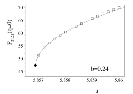
Figure 1: $a$-dependence of the NEP $F_{21,21}({\bf q}={\bf 0})$ in the vicinity of the glass transition point for fixed $b=0.24$ and different values of $a$ (squares). Also shown is the square root fit $47+400\sqrt{a-5.85688}$, leading to the critical values $(a_{c},F_{21,21}^{c}({\bf 0}))$ (black dot). Note the rather large prefactor of the square root.

This has been done by approaching the glass transition point from the glass side. Fig. 1 shows an example where $F_{21,21}({\bf q}={\bf 0})$ is represented as function of $a$ for fixed $b$. The fit with a square root, predicted by MCT for a type B-transition WGoe91 allows to locate the glass transition point $a_{c}(b)$ for fixed $b=0.24$ up to a relative deviation better than $10^{-4}$! The NEP $F_{21,21}({\bf 0})$ for $a=5.857$ (see Fig. 10) deviates less than ten percent from the critical NEP $F^{c}_{21,21}({\bf 0})=47$ at $a_{c}=5.85688$, and no qualitative change is to be expected on further approach towards $a_{c}$.

III.1 Phase diagram

Figure 2: Phase diagram of hard ellipsoids on a sc lattice. Shown is the curve below which the ellipsoids are free rotators (full line with cusp at $X_{0}=1$), the equilibrium phase transition line $\varphi_{\text{eq}}(X_{0})$ from MC simulations (full thin lines), the line $\varphi_{\text{PY}}(X_{0})$ of highest densities to be reached by numerical solution of the OZ/PY equations (dash-dotted lines), the line $\varphi_{\text{extra}}(X_{0})$ for $X_{0}\gtrsim 4$, where the extrapolated OZ/PY results diverge (dotted line) and the MCT glass transition line $\varphi_{c}(X_{0})$ (full thick lines). For $X_{0}\gtrsim 8$, $\varphi_{\text{extra}}(X_{0})$ and $\varphi_{c}(X_{0})$ are almost identical. $\bullet$ denote the five state points for which the nonergodicity parameters presented in Figs. 3-12 were calculated.

The glass transition line $\varphi_{c}(X_{0})$ obtained in this way is shown in Fig. 2. Fig. 2 also contains the equilibrium phase transition line $\varphi_{\text{eq}}(X_{0})$ from MC-simulations, and the line $\varphi_{\text{PY}}(X_{0})$. Also shown is the curve $\varphi_{\text{extra}}(X_{0})$ where the extrapolated OZ/PY static orientational correlators for $X_{0}\gtrsim 4$ at the zone center diverge. $\varphi_{\text{eq}}(X_{0})$ and $\varphi_{\text{PY}}(X_{0})$ were obtained from the corresponding lines $a_{\text{eq}}(b)$ and $a_{\text{PY}}(b)$ of Ref. MRic04 . Finally, the solid line with the cusp at $X_{0}=1$ is the location of all $\varphi(X_{0})$ at which the rotators start to interact.

At $\varphi_{\text{eq}}(X_{0})$, an equilibrium phase transition from a (dynamically) disordered to an orientationally ordered phase occurs. The line $\varphi_{\text{PY}}(X_{0})$ locates the $(X_{0},\varphi)$-pairs for which the iterative numerical procedure to solve the OZ/PY equations becomes unstable. This is associated with some of the maxima of ${\bf S}({\bf q})$ becoming very large, giving evidence of a divergency. Since the $X_{0}$-dependence of $\varphi_{\text{eq}}$ and $\varphi_{\text{PY}}$ is qualitatively similar, this behavior may indicate an equilibrium phase transition, as speculated for a liquid of hard ellipsoids MLe99 . However, in contrast to the latter, the deviation of $\varphi_{\text{PY}}(X_{0})$ from $\varphi_{\text{eq}}(X_{0})$ is much larger, especially for prolate ellipsoids. Using the static correlators from OZ/PY-theory as an input for the calculation of the NEP from Eqs. (22) and (23) we have found a glass transition for $X_{0}\lesssim 0.7$ and $2\lesssim X_{0}\lesssim 2.5$, only. For $0.7\lesssim X_{0}\lesssim 2$ and $X_{0}\gtrsim 4$ the system is ergodic for all $\varphi\leq\varphi_{\text{PY}}(X_{0})$, because the static correlators at the Brillouin zone center and/or edge are too small. Unfortunately, the iterative procedure to solve the OZ/PY equations for $0.7\lesssim X_{0}\lesssim 2$ and $X_{0}\gtrsim 4$ becomes unstable for $\varphi\geq\varphi_{\text{PY}}(X_{0})$. Therefore, we have decided to extrapolate the static correlators to $\varphi\geq\varphi_{\text{PY}}(X_{0})$. This extrapolation is guided by the physical assumption that long range orientational order should occur at the line $\varphi_{\text{extra}}(X_{0})$. It only works for $X_{0}\gtrsim 4$, but not for the gap in between $X_{0}\approx 0.7$ and $X_{0}\approx 2$. Accordingly, the missing glass transition line for $0.7\lesssim X_{0}\lesssim 2$ first of all is based upon the lack of the static input. Since the ergodic and nonergodic phase are separated by a critical line of Type-B transitions WGoe91 ; RSRi54 , $\varphi_{\text{c}}(X_{0})$ can not terminate at $X_{0}\approx 0.7$ or $X_{0}\approx 2$. There exist two possible scenarios for $\varphi_{\text{c}}(X_{0})$ within this gap. First, $\varphi_{\text{c}}(X_{0})$ converges to $\varphi_{\text{c}}(X_{0}=1)$ from above and below $X_{0}=1$, with a possible cusp at $X_{0}=1$. Second, $\varphi_{\text{c}}(X_{0})\to\varphi_{\text{max}}(X_{0}^{\pm})$ for $X_{0}\to X_{0}^{\pm}$ with $0.7\lesssim X_{0}^{-}<1$ and $1<X_{0}^{+}\lesssim 2$, where $\varphi_{\text{max}}(X_{0})$ is the maximum possible volume fraction of an orientationally disordered configuration for given $X_{0}$. The second scenario would imply that there is no glass transition for $X_{0}^{-}\leq X_{0}\leq X_{0}^{+}$, i.e. for ellipsoids which are not sufficiently aspherical.

The non-monotonous behavior of $\varphi_{\text{PY}}(X_{0})$ for prolate ellipsoids with $1<X_{0}\lesssim 4$, which induces a non-monotonicity of $\varphi_{c}(X_{0})$, seems to be an artefact of the PY approximation, as our MC results for hard prolate ellipsoids suggest, though the static orientational correlators from OZ/PY theory are qualitatively correct, anyway MRic04 .

If it is true that the divergence of the PY solutions corresponds to an equilibrium phase transition, this implies that the ideal glass transition is driven by the growth of some $S_{\lambda\lambda^{\prime}}({\bf q})$ at the zone center or/and edge due to the growth of the orientational order, as will be seen in the following figures. This is quite similar to the central peak phenomenon above the equilibrium transition temperature at structural phase transitions of first and second order Bru90 . The central peak can be interpreted as a quasi-nonergodic behavior and has also been described by MCT VLA87 .

The freezing of the $l,l^{\prime}$ odd correlators occurs beyond the $l,l^{\prime}$ even glass transition line and is treated in subsection III.4.

III.2 Critical nonergodicity parameters

The critical NEP $F^{c}_{\lambda\lambda^{\prime}}({\bf q})$ and the normalized critical NEP $f^{c}_{\lambda\lambda^{\prime}}({\bf q})$ together with the static orientational correlators are shown in Figs. 3, 6, 7, 9 and 10 for oblate and prolate ellipsoids, respectively, along the three highly symmetric directions in reciprocal space from the zone center to its edge. For each of the three directions and each matrix element, a separate subfigure is provided, where the indices $lml^{\prime}m^{\prime}$ are displayed at the top of each figure. We have restricted our illustrations to the diagonal elements $l=l^{\prime}=2$, $m=m^{\prime}=0,1,2$ and $l=l^{\prime}=4$, $m=m^{\prime}=0,1,2,3,4$, and the off-diagonal elements $l=2$, $l^{\prime}=4$, $m=m^{\prime}=0,1,2$. By the symmetries of the cubic lattice, these correlators are all real. The scales on the l.h.s. of each tableau belong to $S_{\lambda\lambda^{\prime}}({\bf q})$ and $F^{c}_{\lambda\lambda^{\prime}}({\bf q})$, those on the r.h.s. to $f^{c}_{\lambda\lambda^{\prime}}({\bf q})$. Note the different scales of the axes for different values of $m=m^{\prime}$.

For two pairs $(a,b)$ we also present the corresponding tensorial quantities in real space. Figs. 4 and 8 show log-lin representations of the direct space static orientational correlators $G_{xyz,\lambda\lambda^{\prime}}$ and the corresponding NEP $F^{c}_{xyz,\lambda\lambda^{\prime}}=\lim_{t\to\infty}G_{xyz,\lambda\lambda^{\prime}}(t)$ along lattice directions of high symmetry, i.e. $xyz=00n$, $0nn$ and $nnn$ for $n=0,1,\ldots,8$. Along these directions, all $G_{xyz,\lambda\lambda^{\prime}}$ and $F^{c}_{xyz,\lambda\lambda^{\prime}}$ are real, too, for $\lambda\lambda^{\prime}$ as above. Note that a step $\Delta n=1$ corresponds to different lengths in direct space, namely $1$, $\sqrt{2}$ and $\sqrt{3}$ for the different lattice directions. For each $m=m^{\prime}$ and each lattice direction, a separate figure is provided and a logarithmic plotting has been chosen for positive and negative values of $G_{xyz,\lambda\lambda^{\prime}}$ and $F^{c}_{xyz,\lambda\lambda^{\prime}}$ separately, i.e. the negative values are presented as $-\ln\,|G_{xyz,\lambda\lambda^{\prime}}|$ and $-\ln\,|F^{c}_{xyz,\lambda\lambda^{\prime}}|$, respectively. The values of $xyz,lml^{\prime}m^{\prime}$ are included in each subfigure.

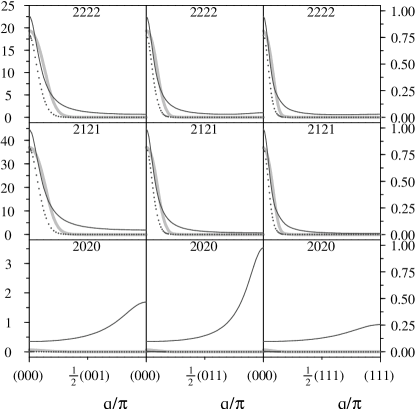
Figure 3: ${\bf q}$-dependence of the nonergodicity parameters $F^{c}_{\lambda\lambda^{\prime}}({\bf q})$ (dotted lines), the normalized ones $f^{c}_{\lambda\lambda^{\prime}}({\bf q})=F^{c}_{\lambda\lambda^{\prime}}({\bf q})\,[\,S_{\lambda\lambda}({\bf q})\,S_{\lambda^{\prime}\lambda^{\prime}}({\bf q})\,]^{-1/2}$ (thick grey lines) and of the static structure factors $S_{\lambda\lambda^{\prime}}({\bf q})$ (solid lines) for $l=l^{\prime}=2$ and $m=m^{\prime}=0,1,2$. Results are shown within the first Brillouin zone along the three highly symmetric reciprocal space directions for oblate ellipsoids with $a=0.08$ and $b=1.412$, i.e. $(X_{0},\varphi)\cong(0.0567,0.0835)$.

Figure 4: The nonergodicity parameters $F^{c}_{xyz,\lambda\lambda^{\prime}}$ in real space (solid circles) and the static orientational density correlators $G_{xyz,\lambda\lambda^{\prime}}$ (squares; dashed lines are a guide to the eye) along the three highly symmetric direct lattice directions for oblate ellipsoids with $a=0.08$ and $b=1.412$, i.e. $(X_{0},\varphi)\cong(0.0567,0.0835)$. Shown are the diagonal correlators for $l=l^{\prime}=2$, $m=m^{\prime}=0,1,2$ and $xyz=00n$, $0nn$ or $nnn$ for $n=0,1,\ldots,8$.

Figure 5: $n$-dependence of the ratio $F^{c}_{00n,21,21}/G_{00n,21,21}$ of the NEP $F^{c}_{00n,21,21}$ and his static counterpart $G_{00n,21,21}$ for oblate ellipsoids with $a=0.08$ and $b=1.412$, i.e. $(X_{0},\varphi)\cong(0.0567,0.0835)$.

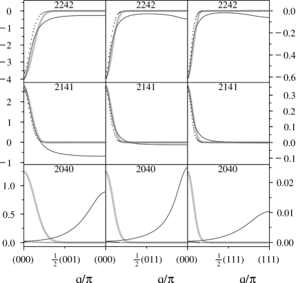
Figure 6: Same as Fig. 3, but for $l=2$, $l^{\prime}=4$.

Figs. 3-6 present the NEP for $l=l^{\prime}=2$ and $l^{\prime}=2,4$ for oblate ellipsoids with $a=0.08$ and $b=1.412$, which yields $(X_{0},\varphi)\cong(0.0567,0.0835)$. In comparison to liquids, the NEP possess less structure in $q$-space. For $l=l^{\prime}=2$, they are maximum exclusively at the zone center. A similar behavior is found for $l\neq l^{\prime}$ (cf. Fig. 6), but here, e.g. for $m=m^{\prime}=2$, minima appear instead of maxima. None of the maxima of the static structure factors $S_{2m,2m}({\bf q})$ and maxima/minima of $S_{2m,4m}({\bf q})$ at the zone boundary persits in the limit $t\to\infty$. Since these maxima belong to alternating orientational density fluctuations, this proves that such alternating local arrangements of the particles do not arrest. This can also be seen in real space. Fig. 4 exhibits the static orientational density correlators $G_{xyz,2m,2m}$ and the $F^{c}_{xyz,2m,2m}$ for $a=0.08$ and $b=1.412$. Indeed, the oscillations in the correlators $G_{00n,20,20}$ and $G_{0nn,20,20}$ vanish completely in the long time limit, while the monotonous decay with $n$ of the $(m=m^{\prime}>0)$-quantities is rather stable, even for infinite time. The almost vanishing of some critical NEP, however, does not require oscillations in the corresponding $G_{xyz,\lambda\lambda^{\prime}}$, as can be seen from $G_{nnn,20,20}$ and $F^{c}_{nnn,20,20}$. Another remarkable feature is the behavior at small $n$, particularly at $n=0$. Fig. 4 demonstrates that, e.g., the magnitude of $F^{c}_{000,2m,2m}$ for $m=1,2$ is only a few percent or even less of that of $G_{000,2m,2m}$. Fig. 5 shows that the ratio $F^{c}_{00n,21,21}/G_{00n,21,21}$ becomes very small as $n$ is lowered. A similar behavior has been found for all values $(X_{0},\varphi)$ on the glass transition lines we have investigated. The dips in $F^{c}_{xyz,\lambda\lambda^{\prime}}/G_{xyz,\lambda\lambda^{\prime}}$ at $n=0$ demonstrate that the relaxation of the “self” part of the orientational correlators is practically not arrested by an orientational cage.

Moving for oblate ellipsoids along the glass transition line towards the spherical limit $X_{0}=1$, no qualitatively new behavior of the critical NEP is found, but it resembles always the characteristics of Figs. 3 and 6. However, this picture will change as we turn for oblate ellipsoids into the glass phase, as will be seen in subsection III.3.

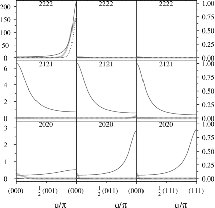
Figure 7: Same as Fig. 3, but for prolate ellipsoids with $a=1.4524$ and $b=0.72$, i.e. $(X_{0},\varphi)\cong(2.02,0.394)$.

Figure 8: Same as Fig. 4, but for prolate ellipsoids with $a=1.4524$ and $b=0.72$, i.e. $(X_{0},\varphi)\cong(2.02,0.394)$.

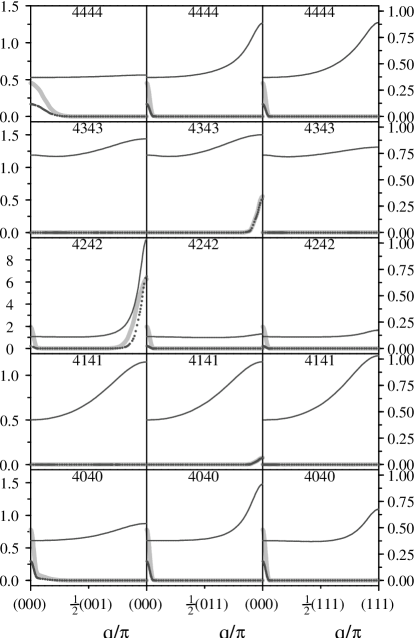
Figure 9: Same as Fig. 3, but for prolate ellipsoids with $a=1.4524$ and $b=0.72$, i.e. $(X_{0},\varphi)\cong(2.02,0.394)$, and for $l=l^{\prime}=4$, $m=m^{\prime}=0,1,2,3,4$.

The $q$-dependence of the critical NEP for prolate ellipsoids is sensitive on the shape of the ellipsoids (see Figs. 7, 9 and 10). The reader should note the higher values of the maxima in $S_{\lambda\lambda^{\prime}}({\bf q})$, which are necessary to get a glass transition, compared to the corresponding correlators for oblate ellipsoids. Let us have a closer look at prolate ellipsoids with $a=1.4524$ and $b=0.72$, i.e. $(X_{0},\varphi)\cong(2.02,0.394)$. Fig. 7 shows that the structural arrest of these ellipsoids is completely different from that of oblate ones. The huge peak in $F^{c}_{22,22}({\bf q}=(0,0,\pi))$ at the zone boundary has a height of 157 and dominates the transition. Since this peak belongs to a wavelength of period two, it leads to strong frozen oscillations in the orientational density fluctuations on the lattice, as can be seen in direct space from Fig. 8. Note that for the correlators $F^{c}_{00n,21,21}$ almost no decay exists if $n$ is increased. Again, like for oblate ellipsoids, the frozen $F^{c}_{xyz,20,20}$ seem to play a special role, since they are much weaker than the NEP for $m=m^{\prime}>0$. Fig. 9 shows the diagonal correlators for $l=l^{\prime}=4$. Note the very small scale for the static structure factors and NEP, in comparison with Fig. 7. Fig. 9 shows other interesting features of the MCT results for molecular crystals: besides the appearance of simultaneous maxima of the normalized NEP at the zone center and its boundary (see $f_{42,42}({\bf q})$ along the fourfold reciprocal space direction), the rule that the normalized NEP in reciprocal space are in phase with the corresponding static correlators GS1992 is violated.

Finally, it must be said that the static structure factors for ellipsoids with $a=1.4524$, $b=0.72$ have been calculated by OZ/PY theory. But MC results MRic04 for other values of $(a,b)$ in the vicinity of these parameters show that OZ/PY overestimates the maxima at the zone bondary in this region of the phase diagram. Therefore, the interpretation of Figs. 7-9 should be taken with some caution. Perhaps this overestimation is the indirect cause for the dip in $\varphi_{\text{PY}}(X_{0})$ for $2\lesssim X\lesssim 4$ (see Fig. 2). Why OZ/PY fails in this region of ellipsoids is currently unknown.

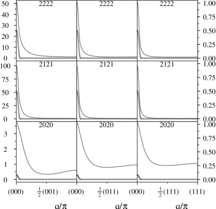
Figure 10: Same as Fig. 3, but for prolate ellipsoids with $a=5.857$ and $b=0.24$, i.e. $(X_{0},\varphi)\cong(24.4,0.177)$.

As we turn to very elongated prolate ellipsoids, the transition scenario becomes simpler again. Fig. 10 for $a=5.857$ and $b=0.24$ [yielding $(X_{0},\varphi)\cong(24.4,0.177)$] serve as an illustration. The behavior of the $(l=l^{\prime}=2)$-NEP with peaks at the zone center reminds one of the NEP for flat oblate ellipsoids (see Fig. 3). This means that for long prolate ellipsoids only nematic-like orientational fluctuations may freeze. Such an extreme narrowness of the peaks at ${\bf q}={\bf 0}$ as seen in Fig. 10 is observed for prolate ellipsoids with $X_{0}\gtrsim 8$ only, indicating the huge spatial extension of the frozen nematic-like fluctuations.

III.3 Nonergodicity parameters in the glass phase

In this subsection, we show by means of two examples how the NEP change in comparison to the critical NEP on moving slightly into the glass phase. The corresponding pairs $(X_{0},\varphi)$ are indicated in Fig. 2, too.

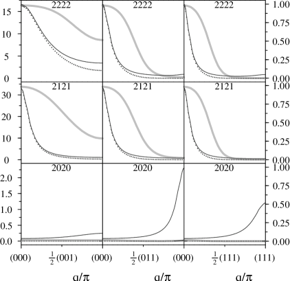
Figure 11: Same as Fig. 3, but for oblate ellipsoids with $a=0.78$ and $b=1.1$, i.e. $(X_{0},\varphi)\cong(0.709,0.494)$, above the glass line.

For densely packed oblate ellipsoids with $a=0.78$ and $b=1.1$, i.e. $(X_{0},\varphi)\cong(0.709,0.494)$ in the glass phase, the prototypical behavior of the critical NEP for oblate ellipsoids on the glass transition line shown in Figs. 3 and 6 is clearly changed, as can be seen from Fig. 11 . Now, the Gaussian-like shape of the normalized NEP is much broader, indicating an enhanced arrest of orientational density fluctuations for ${\bf q}\neq{\bf 0}$, which is expected due to the high packing fraction. This leads to a deviation of the frozen orientational correlators in direct space from the exclusive monotonous decay, which is present almost everywhere along the glass transition line for oblate ellipsoids. For example, the frozen $F_{00n,20,20}$ for the $(a,b)$-pair of Fig. 11 (not shown here) have weak oscillations, reminiscent of the strong oscillations being present in the associated static $G_{00n,20,20}$.

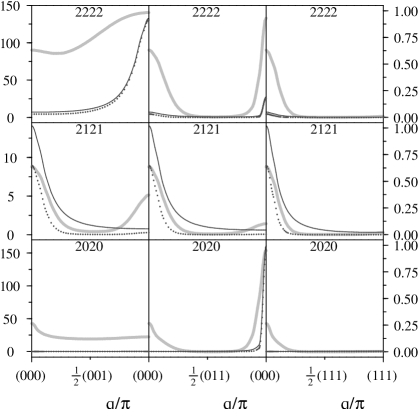
Figure 12: Same as Fig. 3, but for prolate ellipsoids with $a=1.7$ and $b=0.66$, i.e. $(X_{0},\varphi)\cong(2.58,0.389)$, above the glass line.

Considering prolate ellipsoids with $a=1.7$ and $b=0.66$, i.e. $(X_{0},\varphi)\cong(2.58,0.389)$, slightly above the glass transition line, many different patterns of behavior occur in the NEP, as can be seen from Fig. 12. This figure can directly be compared with Fig. 7, since the ellipsoids for both figures have almost the same packing fraction. Again, for one and the same NEP there partly exist simultaneous maxima at the zone center and its boundary. Accordingly, in the limit of long times, we have frozen density-density correlators with either oscillatory or monotonous behavior, depending on $\lambda\lambda^{\prime}$.

III.4 Glass transition of the $l,l^{\prime}$ odd correlators

So far we have discussed the NEP for $l,l^{\prime}$ even. For $l,l^{\prime}$ odd only the “self” part of the NEP is nonzero. It is useful to investigate the normalized, rotationally invariant “self” part of the NEP, i.e.

$$f^{(s)}_{l}=\frac{\sum_{m=-l}^{l}F_{000,lm,lm}}{\sum_{m=-l}^{l}G_{000,lm,lm}}\,.$$ (26)

Values for $f^{(s)}_{l}$ are given in Table 1 for those pairs $(a,b)$ for which the glass transition has been found for $l,l^{\prime}$ odd. For comparison, the $f^{(s)}_{l}$ for $l$ even are given in Table 1, too. The relation

$$f^{(s)}_{l}<f^{(s)}_{l^{\prime}}\,,\quad\quad l>l^{\prime}\,,$$ (27)

which is similar to

$$f^{c}(q)<f^{c}(q^{\prime})\,,\quad\quad q>q^{\prime}$$ (28)

for simple liquids, seems to be fulfilled for even and odd $l$ separately. Note that the pairs $(a,b)$ in Table 1 are located in the glass phase for $l,l^{\prime}$ even.

$(a,b)$	$l=1$	$l=2$	$l=3$	$l=4$
$(0.776,1.1)$	$0.203$	$0.208$	$0.124$	$0.106$
$(0.778,1.1)$	$0.406$	$0.268$	$0.262$	$0.143$
$(0.78,1.1)$	$0.546$	$0.333$	$0.371$	$0.185$
$(1.7,0.66)$	$3.00\times 10^{-2}$	$0.197$	$8.14\times 10^{-3}$	$3.93\times 10^{-2}$

Table 1: Selected normalized NEP $f^{(s)}_{l}$ of the “self” part of the orientational density-density correlation function (see Eqs. (24), (25)).

IV Discussion and conclusions

We have extended the mode coupling theory (MCT) for liquids to molecular crystals. The natural choice is the use of tensorial correlators, instead of correlators defined in a site-site representation SHCH98 . This leads for the dynamical correlators $S_{\lambda\lambda^{\prime}}({\bf q},t)$ to an integro-differential equation of second order in time. Truncating $l$ at $l_{\text{max}}$, this set of equations is equivalent to the corresponding equation for a multi-component liquid of isotropic particles (for binary systems see, e.g., VG ). The memory kernel is approximated in the framework of MCT. The main differences to liquids are (i) the occurrence of Umklapp processes, if the sum of the wave vectors ${\bf q}_{1}$, ${\bf q}_{2}$ of the orientational density modes $\delta\rho_{\lambda_{1}}({\bf q}_{1})$ and $\delta\rho_{\lambda_{2}}({\bf q}_{2})$ is outside of the first Brillouin zone, (ii) besides the static two-point orientational correlators $S_{\lambda\lambda^{\prime}}({\bf q})$ the need of the one-molecule orientational density $\rho^{(1)}(\Omega)$ as an input for the vertices of the memory kernel and (iii) the anisotropy of the static orientational current density correlators $J_{\lambda\lambda^{\prime}}$ which do not cancel completely from the memory kernel $m_{\lambda\lambda^{\prime}}({\bf q},t)$. Nevertheless, the factor $k_{B}T/I$ of $J_{\lambda\lambda^{\prime}}$ drops out. Accordingly, the glassy dynamics and the ideal glass transition does not exhibit inertia effects, i.e. they are independent on $I$, the moment of inertia. Additionally, for rigid lattices, all $l,l^{\prime}=0$ tensorial correlators vanish and can be skipped, due to the lack of TDOF.

In order to discuss this set of MCT-equations for molecular crystals we have chosen hard ellipsoids of revolution with aspect ratio $X_{0}=a/b$ fixed with their centers of mass at the sites of a sc-lattice with lattice constant equal to one. Increasing the size of the ellipsoids, which is equivalent to a decrease of the lattice constant, results in an increase of steric hindrance and finally in an orientational glass transition at the MCT-glass transition line $\varphi_{c}(X_{0})$ shown in Fig. 2 for oblate and prolate ellipsoids. Since this orientational glass transition is mainly driven by the growth of $S_{\lambda\lambda^{\prime}}({\bf q})$ at the zone center or/and the zone edge, its origin lies in the growth of the orientational order close to but below the equilibrium phase transition line from OZ/PY theory. This is quite similar to what has been found for a liquid of hard ellipsoids MLeRS00 if the aspect ratio becomes larger than about 2 or smaller than about $\frac{1}{2}$. However, there is a difference between the molecular liquid (of ellipsoids) and the molecular crystal. Whereas the former already undergoes a glass transition for $X_{0}>2$ or $X_{0}<\frac{1}{2}$ when $S_{2m,2m}({\bf 0})$ is of order one, it must be $S_{2m,2m}({\bf 0})$ of order 10 for oblate (cf. Fig. 3) or even order 100 for prolate ellipsoids (cf. Fig. 7). This proves that the translational degrees of freedom of the liquid still have a strong influence on the glass formation, although they are not primarily responsible for the transition for $X_{0}>2$ and $X_{0}<\frac{1}{2}$. This finding is consistent with results found from a MD simulation for difluorotetrachloroethane in its supercooled liquid and plastic crystal phase FAffpri . For both phases, the glass transition temperatures $T_{c}^{\text{liquid}}$ and $T_{c}^{\text{plastic crystal}}$ were determined. That $T_{c}^{\text{liquid}}\cong 139\mathrm{K}>T_{c}^{\text{plastic crystal}}\cong 129\mathrm{K}$ implies that the translational degrees of freedom of a liquid enhance the glass formation which might be related to a facilitated cage formation for systems where the center of mass of the particles can move freely.

Comparing $S_{\lambda\lambda^{\prime}}({\bf q})$ on the glass transition line for oblate (Figs. 3 and 6) with prolate ellipsoids (Figs. 7 and 9-10) already shows that the tendency to an orientational glass formation for oblate ellipsoids is larger than for prolate ones. This can also be seen from Fig. 2 since the distance $\varphi_{\text{PY}}(X_{0})-\varphi_{c}(X_{0})$ is large for very flat oblate ellipsoids, only. This difference may be explained as follows. If we fix the length $a$ of prolate ellipsoids and decrease their thickness $b$ to zero, then the excluded volume interaction becomes zero. Particularly, the static correlators become trivial, which leads to vanishing vertices and consequently to a disappearance of the MCT glass transition. If on the other hand we fix the diameter $b$ of the oblate ellipsoids and decrease their thickness $a$ to zero the excluded volume interaction still exists for $a=0$. This seems to be an important difference between oblate and prolate particles.

From the solution of the MCT equations for $t\to\infty$ we obtained results for the critical NEP $F_{\lambda\lambda^{\prime}}^{c}({\bf q})$ and the corresponding normalized ones, $f_{\lambda\lambda^{\prime}}^{c}({\bf q})$, as well as NEP deeper in the glass. Due to the lattice translational invariance, ${\bf q}$ can be restricted to the first Brillouin zone. Within this zone the critical NEP do not have much structure. Almost all of them either exhibit a maximum (or minimum for $l\neq l^{\prime}$) at the zone center and/or at its edge, depending on $\lambda\lambda^{\prime}$ and the direction of ${\bf q}$. However, going deeper into the glass and varying the ellipsoid shape, i.e. $X_{0}$ and/or $\varphi$, leads to significant changes in the ${\bf q}$-dependence especially of the normalized NEP, as demonstrated in Figs. 11 and 12.

The MD-simulations for cyanoadamantane AffDes99 and chloradamantane AffCoDe01 reveal quite similar glassy dynamics as found for supercooled liquids WGoe98 ; WGoe99 ; KBin03 . Particularly, the authors of Refs. AffDes99 ; AffCoDe01 stress that their molecular crystals can be supercooled and that the relaxational dynamics is consistent with MCT predictions, at least where this has been checked AffDes99 ; AffCoDe01 . Since both model systems exhibit tremendous slowing down in the supercooled regime an orientational glass transition or at least a crossover from ergodic to quasi-nonergodic dynamics must also occur in the supercooled phase. This is different from what we have found for the hard ellipsoids. In our case the glass transition line is located within the dynamically disordered equilibrium phase of PY theory, which itself is a consequence of the static input taken from PY theory. It would be very interesting to insert the static correlators  from the MD simulations in the supercooled phase into our MCT equations and to check whether one obtains a glass transition. The investigation of hard ellipsoids on the sc lattice has demonstrated that the magnitude of the extrema in $S_{\lambda\lambda^{\prime}}({\bf q})$ at the zone center or/and edge must be rather large (at least for prolate particles). It is not obvious that the simulational results in the supercooled phase fulfill this criterion. Of course, it could be that the average height of $S_{\lambda\lambda^{\prime}}({\bf q})$ in $q$-space is much larger than for the ellipsoids such that large maxima/minima of $S_{\lambda\lambda^{\prime}}({\bm{q}})$ at the zone center and/or edge are not really necessary. We hope that these questions can be answered in future.

To conclude, we have shown that MCT can be derived for molecular crystals, as well. Whether or not the MCT approximation (which mainly consists of the factorization of a time dependent four point correlator) is also a reasonable approximation for molecular crystals as it is for glass-forming liquids has to be investigated by comparison of the results from present MCT for molecular crystals with simulational and experimental results. As already mentioned above our conventional MCT approach will become worse if the thickness of prolate particles becomes small. In that case it is the entanglement which is responsible for glassy dynamics CRenLoe97 ; SPOb97 . This requires a different theoretical description, as recently discussed RSGZ03 ; RSAd04 .

Appendix A Calculation of $J_{\lambda\lambda^{\prime}}({\bf q})\equiv J_{\lambda\lambda^{\prime}}$

Substituting the $\lambda$-Fourier transform $j_{\lambda}({\bf q})$ of $j_{n}(\Omega)$ (Eq. (6)) into Eq. (11) yields

$$J_{\lambda\lambda^{\prime}}({\bf q})=\frac{4\pi}{N}\,i^{l^{\prime}-l}\,\sum_{nn^{\prime}}\,\text{e}^{i{\bf q}\cdot{\bf x}_{nn^{\prime}}}\,\times$$

$$\times\,\big{\langle}\,({\bm{\omega}}_{n}\cdot\hat{{\bf L}}_{\Omega_{n}}Y_{\lambda}(\Omega_{n}))^{*}\,({\bm{\omega}}_{n^{\prime}}\cdot\hat{{\bf L}}_{\Omega_{n^{\prime}}}Y_{\lambda^{\prime}}(\Omega_{n^{\prime}}))\,\big{\rangle}\,.$$ (29)

Since $\bm{\omega}_{n}\cdot\hat{{\bf L}}_{\Omega_{n}}=\bm{\omega}^{\prime}_{n}\cdot\hat{{\bf L}}^{\prime}_{\Omega_{n}}$ (where the primed quantities refer to the body fixed frame) we get for the canonical average in Eq. (A) in close analogy to molecular liquids RSTS97

$$\big{\langle} \ldots\big{\rangle}=\sum_{\alpha\alpha^{\prime}}\,\big{\langle}\omega_{n}^{\prime\alpha}\omega_{n^{\prime}}^{\prime\alpha^{\prime}}\big{\rangle}\,\big{\langle}\,(\hat{L^{\prime}}_{\Omega_{n}}^{\alpha}\,Y_{\lambda}(\Omega_{n}))^{*}\,(\hat{L^{\prime}}_{\Omega_{n^{\prime}}}^{\alpha^{\prime}}\,Y_{\lambda^{\prime}}(\Omega_{n^{\prime}}))\,\big{\rangle}\,$$

$$=\sum_{\alpha\alpha^{\prime}}\,\frac{kT}{I}\,\delta_{nn^{\prime}}\delta_{\alpha\alpha^{\prime}}\,\big{\langle}\,(\hat{L^{\prime}}_{\Omega_{n}}^{\alpha}Y_{\lambda}(\Omega_{n}))^{*}\,(\hat{L^{\prime}}_{\Omega_{n^{\prime}}}^{\alpha^{\prime}}Y_{\lambda^{\prime}}(\Omega_{n^{\prime}}))\,\big{\rangle}\,,$$ (30)

where, $\alpha=x,y,z$ are the cartesian components in the body fixed frame. This leads to

$$J_{\lambda\lambda^{\prime}}({\bf q}) =4\pi\,\frac{kT}{I}\,i^{l^{\prime}-l}\,\big{\langle}\,(\hat{{\bf L}}_{\Omega_{n}}Y_{\lambda}(\Omega_{n}))^{*}\,\cdot\,(\hat{{\bf L}}_{\Omega_{n}}Y_{\lambda^{\prime}}(\Omega_{n}))\,\big{\rangle}\,,$$ (31)

which is ${\bf q}$- and $n$-independent, and can therefore be evaluated for arbitrary $n$. Using $\hat{L}^{\alpha}_{\Omega}\,Y_{lm}(\Omega)=\sum_{m^{\prime}=-l}^{l}L^{\alpha}_{l,mm^{\prime}}Y_{lm^{\prime}}(\Omega)$ and the product rule for the spherical harmonics and substituting the explicit expression for $L^{\alpha}_{l,mm^{\prime}}$ we get with $c(l,l^{\prime},l^{\prime\prime})$ as in (47)

$$J_{\lambda\lambda^{\prime}}({\bf q})=\> 4\pi\,\frac{kT}{I}\,i^{l^{\prime}-l}\,(-1)^{m}\,\sum_{\lambda^{\prime\prime}}\Big{[}\,mm^{\prime}\,C(ll^{\prime}l^{\prime\prime},-mm^{\prime}m^{\prime\prime})$$

$$-\frac{1}{2}\sqrt{l(l+1)-m(m+1)}\,\sqrt{l^{\prime}(l^{\prime}+1)-m^{\prime}(m^{\prime}+1)}\;C(ll^{\prime}l^{\prime\prime},-m-1,m^{\prime}+1,m^{\prime\prime})$$

$$-\frac{1}{2}\sqrt{l(l+1)-m(m-1)}\,\sqrt{l^{\prime}(l^{\prime}+1)-m^{\prime}(m^{\prime}-1)}\;C(ll^{\prime}l^{\prime\prime},-m+1,m^{\prime}-1,m^{\prime\prime})\,\Big{]}\,c(ll^{\prime}l^{\prime\prime})\,\big{\langle}\,Y_{\lambda^{\prime\prime}}\,\big{\rangle}\,.$$ (32)

This expression strongly simplifies since

$$[\cdots]\,c(ll^{\prime}l^{\prime\prime}) =-\frac{1}{2}\,\sqrt{l(l+1)}\,\sqrt{l^{\prime}(l^{\prime}+1)}\,\left[\frac{(2l+1)(2l^{\prime}+1)}{4\pi\,(2l^{\prime\prime}+1)}\right]^{\frac{1}{2}}\big{\{}C(ll^{\prime}l^{\prime\prime},1-10)+C(ll^{\prime}l^{\prime\prime},-110)\big{\}}\,C(ll^{\prime}l^{\prime\prime},-mm^{\prime}m^{\prime\prime})\,.$$ (33)

This leads to the final result

$$J_{\lambda\lambda^{\prime}}({\bf q}) =4\pi\,\frac{kT}{I}\,i^{l^{\prime}-l}\,(-1)^{m+1}\,\frac{1}{2}\,\sqrt{l(l+1)}\,\sqrt{l^{\prime}(l^{\prime}+1)}\,\times$$

$$\times\sum_{\lambda^{\prime\prime}}\left[\frac{(2l+1)(2l^{\prime}+1)}{4\pi\,(2l^{\prime\prime}+1)}\right]^{\frac{1}{2}}\big{\{}C(ll^{\prime}l^{\prime\prime},1-10)+C(ll^{\prime}l^{\prime\prime},-110)\big{\}}\,C(ll^{\prime}l^{\prime\prime},-mm^{\prime}m^{\prime\prime})\,\big{\langle}\,Y_{\lambda^{\prime\prime}}\,\big{\rangle}\,.$$ (34)

Note that $\langle Y_{\lambda}\rangle$ is given by

$$\big{\langle}\,Y_{\lambda}\,\big{\rangle}=\int\,\text{d}\Omega\,\rho^{(1)}(\Omega)\,Y_{\lambda}(\Omega)=(-i)^{l}\,\rho^{(1)}_{\lambda}\,,$$ (35)

i.e. $J_{\lambda\lambda^{\prime}}({\bf q})\equiv J_{\lambda\lambda^{\prime}}$ only involves the $\lambda$-transform of $\rho^{(1)}(\Omega)$.

Appendix B Mode coupling approximation

In this appendix we shortly describe the mode coupling approximation leading to the results presented by Eqs. (15)-(19).

The derivation of the Mori-Zwanzig equation is standard by using the projectors onto the slow variables $\delta\rho_{\lambda}({\bf q})$ and $j_{\lambda}({\bf q})$,

$$P_{\rho} =\frac{4\pi}{N}\,\sum_{\lambda\lambda^{\prime}}\!^{\prime}\,\,\big{|}\,\delta\rho_{\lambda}({\bf q})\,\big{\rangle}\,({\bf S}^{-1}({\bf q}))_{\lambda\lambda^{\prime}}\,\big{\langle}\,\delta\rho^{*}_{\lambda^{\prime}}({\bf q})\,\big{|}\,,$$ (36)

$$P_{j} =\frac{4\pi}{N}\,\sum_{\lambda\lambda^{\prime}}\!^{\prime}\,\,\big{|}\,j_{\lambda}({\bf q})\,\big{\rangle}\,({\bf J}^{-1})_{\lambda\lambda^{\prime}}\,\big{\langle}\,j^{*}_{\lambda^{\prime}}({\bf q})\,\big{|}\,.$$ (37)

The prime on sums denotes summation such that $l,l^{\prime}>0$. The projector $Q$ in Eq. (14) is the given by

$$Q=1-P_{\rho}-P_{j}\,.$$ (38)

In order to approximate $M_{\lambda\lambda^{\prime}}({\bf q},t)$ Eq. (14) we introduce the projector onto pairs of orientational density modes:

$$\mathcal{P}=\sum_{\begin{subarray}{c}{\bf q}_{1}{\bf q}_{1}^{\prime},{\bf q}_{2}{\bf q}_{2}^{\prime}\\ \in\,\text{1.BZ}\end{subarray}}\;\sum_{\lambda_{1}\lambda_{1}^{\prime}\lambda_{2}\lambda_{2}^{\prime}}^{\prime}\;\;\big{|}\,\delta\rho_{\lambda_{1}}({\bf q}_{1})\,\delta\rho_{\lambda_{1}^{\prime}}({\bf q}_{1}^{\prime})\,\big{\rangle}\,\times$$

$$\times\,g_{\lambda_{1}\lambda_{1}^{\prime};\lambda_{2}\lambda_{2}^{\prime}}({\bf q}_{1}{\bf q}_{1}^{\prime},{\bf q}_{2}{\bf q}_{2}^{\prime})\;\big{\langle}\,\delta\rho^{*}_{\lambda_{2}}({\bf q}_{2})\,\delta\rho^{*}_{\lambda_{2}^{\prime}}({\bf q}_{2}^{\prime})\,\big{|}\,,$$ (39)

where $(g_{\lambda_{1}\lambda^{\prime}_{1},\lambda_{2}\lambda^{\prime}_{2}}({\bf q}_{1}{\bf q}^{\prime}_{1};{\bf q}_{2}{\bf q}^{\prime}_{2}))$ is the inverse of the static four-point correlation matrix $(\langle\,\delta\rho^{*}_{\lambda_{1}}({\bf q}_{1})\,\delta\rho^{*}_{\lambda^{\prime}_{1}}({\bf q}^{\prime}_{1})\,\times$ $\times\,\delta\rho_{\lambda_{2}}({\bf q}_{2})\,\delta\rho_{\lambda^{\prime}_{2}}({\bf q}^{\prime}_{2})\,\rangle)$. We use the approximation

$$g_{\lambda_{1}\lambda_{1}^{\prime};\lambda_{2}\lambda_{2}^{\prime}}({\bf q}_{1}{\bf q}_{1}^{\prime},{\bf q}_{2}{\bf q}_{2}^{\prime})\approx\frac{1}{4}\,\left(\frac{4\pi}{N}\right)^{2}\times$$ (40)

$$\times\Big{[}\,\delta_{{\bf q}_{1}{\bf q}_{2}}\,\delta_{{\bf q}_{1}^{\prime},{\bf q}_{2}^{\prime}}\,({\bf S}^{-1}({\bf q}_{1}))_{\lambda_{1}\lambda_{2}}\,({\bf S}^{-1}({\bf q}_{2}))_{\lambda^{\prime}_{1}\lambda^{\prime}_{2}}+(1\leftrightarrow 2)\,\Big{]},$$

which is consistent with the mode coupling approximation of $M_{\lambda\lambda^{\prime}}({\bf q},t)$ for $t=0$ (see Eq. (B)).

The mode coupling approximation consists of two main steps. First, the fluctuating force is approximated

$$Q\;\big{|}\,\mathcal{L}j_{\lambda}({\bf q})\,\big{\rangle}\approx\mathcal{P}Q\;\big{|}\,\mathcal{L}j_{\lambda}({\bf q})\big{\rangle}\,.$$ (41)

Substituting (41) into Eq. (14) leads to a time-dependent four-point correlator, which in a second approximation is factorized. For ${\bf q}_{1},{\bf q}^{\prime}_{1},{\bf q}_{2},{\bf q}^{\prime}_{2}\in$ 1.BZ we have

$$\big{\langle}\,\delta\rho^{*}_{\lambda_{1}}({\bf q}_{1})\,\delta\rho^{*}_{\lambda_{1}^{\prime}}({\bf q}_{1}^{\prime})\,\big{|}\,Q\,\text{e}^{-i\,Q\,\mathcal{L}\,Q\,t}\,Q\,\,\big{|}\,\delta\rho_{\lambda_{2}}({\bf q}_{2})\,\delta\rho_{\lambda_{2}^{\prime}}({\bf q}_{2}^{\prime})\,\big{\rangle}\approx$$

$$\frac{N^{2}}{(4\pi)^{2}}\,\Big{[}\,\,\delta_{{\bf q}_{1},{\bf q}_{2}}\,\delta_{{\bf q}_{1}^{\prime},{\bf q}_{2}^{\prime}}\,S_{\lambda_{1}\lambda_{2}}({\bf q}_{1},t)\,S_{\lambda_{1}^{\prime}\lambda_{2}^{\prime}}({\bf q}_{2},t)+(1\leftrightarrow 2)\,\Big{]}.$$ (42)

With these approximations we obtain

$$M_{\lambda\lambda^{\prime}} ({\bf q},t)\approx\frac{1}{2}\,\left(\frac{4\pi}{N}\right)^{3}\,\sum\limits_{{\bf q}_{1}{\bf q}_{2}\atop\in\text{1.BZ}}\;\sum\limits_{\begin{subarray}{c}\lambda_{1}\lambda_{2}\lambda_{3}\lambda_{4}\\ \lambda_{1}^{\prime}\lambda_{2}^{\prime}\lambda_{3}^{\prime}\lambda_{4}^{\prime}\end{subarray}}^{\prime}$$

$$\times\big{\langle}\,(\mathcal{L}\,j_{\lambda}({\bf q}))^{*}\,\big{|}\,Q\,\big{|}\,\delta\rho_{\lambda_{1}}({\bf q}_{1})\,\delta\rho_{\lambda_{2}}({\bf q}_{2})\,\big{\rangle}\,\times$$

$$\times({\bf S}^{-1}({\bf q}_{1}))_{\lambda_{1}\lambda_{3}}\,({\bf S}^{-1}({\bf q}_{2}))_{\lambda_{2}\lambda_{4}}\times$$

$$\times S_{\lambda_{3}\lambda^{\prime}_{3}}({\bf q}_{1},t)\,S_{\lambda_{4}\lambda^{\prime}_{4}}({\bf q}_{2},t)\,\times$$

$$\times({\bf S}^{-1}({\bf q}_{1}))_{\lambda_{3}^{\prime}\lambda_{1}^{\prime}}\,({\bf S}^{-1}({\bf q}_{2}))_{\lambda_{4}^{\prime}\lambda_{2}^{\prime}}\times$$

$$\times\big{\langle}\,\delta\rho^{*}_{\lambda_{2}^{\prime}}({\bf q}_{2})\,\delta\rho^{*}_{\lambda_{1}^{\prime}}({\bf q}_{1})\,\big{|}\,Q\,\big{|}\,\mathcal{L}\,j_{\lambda^{\prime}}({\bf q})\,\big{\rangle}\,.$$ (43)

Appendix C Calculation of $\langle\,(\mathcal{L}j_{\lambda}({\bf q}))^{*}\,|\,Q\,|\,\delta\rho_{\lambda_{1}}({\bf q}_{1})\,\delta\rho_{\lambda_{2}}({\bf q}_{2})\,\rangle$

This correlator is calculated quite similar to simple WGoe91 and molecular liquids RSTS97 ; RSP02 ; LFa99 by using Eq. (38) and $P_{j}\,|\,\delta\rho_{\lambda_{1}}({\bf q}_{1})\,\delta\rho_{\lambda_{2}}({\bf q}_{2})\,\rangle=0$, due to time reversal symmetry. Then we get

$$\big{\langle}\,(\mathcal{L}j_{\lambda}({\bf q}))^{*}\,\big{|}\,Q\,\big{|}\,\delta\rho_{\lambda_{1}}({\bf q}_{1})\,\delta\rho_{\lambda_{2}}({\bf q}_{2})\,\big{\rangle}=$$

$$=\big{\langle}\,(\mathcal{L}j_{\lambda}({\bf q}))^{*}\,\delta\rho_{\lambda_{1}}({\bf q}_{1})\,\delta\rho_{\lambda_{2}}({\bf q}_{2})\,\big{\rangle}$$

$$-\big{\langle}\,(\mathcal{L}j_{\lambda}({\bf q}))^{*}\,\big{|}\,P_{\rho}\,\big{|}\,\delta\rho_{\lambda_{1}}({\bf q}_{1})\,\delta\rho_{\lambda_{2}}({\bf q}_{2})\,\big{\rangle}\,.$$ (44)

The first term on the r.h.s. of Eq. (C) is easily rewritten by taking into account the hermiticity of ${\cal L}$ and the continuity equation Eq. (4) and Eq. (6). This leads to

$$\big{\langle}\,(\mathcal{L}j_{\lambda}({\bf q}))^{*}\,\delta\rho_{\lambda_{1}}({\bf q}_{1})\,\delta\rho_{\lambda_{2}}({\bf q}_{2})\,\big{\rangle}=$$

$$=\big{\langle}\,j^{*}_{\lambda}({\bf q})\,j_{\lambda_{1}}({\bf q}_{1})\,\delta\rho_{\lambda_{2}}({\bf q}_{2})\,\big{\rangle}+(1\leftrightarrow 2)\,.$$ (45)

Substituing the $\lambda$-Fourier transform of $\delta\rho_{n}(\Omega)$ and $j_{n}(\Omega)$ into the r.h.s of Eq. (C) we arrive at

$$\big{\langle}\,j^{*}_{\lambda}({\bf q})\,j_{\lambda_{1}}({\bf q}_{1})\,\delta\rho_{\lambda_{2}}({\bf q}_{2})\,\big{\rangle}= \frac{N}{4\pi}\,\frac{kT}{I}\,\sum_{{\bf Q}}\delta_{{\bf q}_{1}+{\bf q}_{2},{\bf q}+{\bf Q}}\sum_{\lambda^{\prime\prime}}\!^{\prime}\;i^{l_{1}+l^{\prime\prime}-l}\,\,(-1)^{m+m^{\prime\prime}}\,\bigg{[}\,mm_{1}\,C(ll_{1}l^{\prime\prime},-mm_{1}-m^{\prime\prime})$$

$$-\frac{1}{2}\sqrt{l(l+1)-m(m+1)}\, \sqrt{l_{1}(l_{1}+1)-m_{1}(m_{1}+1)}\;C(ll_{1}l^{\prime\prime},-m-1,m_{1}+1,-m^{\prime\prime})$$

$$-\frac{1}{2}\sqrt{l(l+1)-m(m-1)}\, \sqrt{l_{1}(l_{1}+1)-m_{1}(m_{1}-1)}\;C(ll_{1}l^{\prime\prime},-m+1,m_{1}-1,-m^{\prime\prime})\,\bigg{]}\,c(ll_{1}l^{\prime\prime})\,S_{\lambda^{\prime\prime}\lambda_{2}}({\bf q}_{2})$$ (46)

with

$$c(ll^{\prime}l^{\prime\prime})=\left[\frac{(2l+1)(2l^{\prime}+1)}{4\pi\,(2l^{\prime\prime}+1)}\right]^{\frac{1}{2}}C(ll^{\prime}l^{\prime\prime},000)\,.$$ (47)

Here we have used the product rule for the spherical harmonics and the factorization of canonic integrals as in Eq. (A). The second term on the r.h.s. of Eq. (C) is rewritten by using $P_{\rho}$ from Eq. (36) and again the hermiticity of ${\cal L}$, as well as the continuity equation:

$$\big{\langle}\,(\mathcal{L} j_{\lambda}({\bf q}))^{*}\,\big{|}\,P_{\rho}\,\big{|}\,\delta\rho_{\lambda_{1}}({\bf q}_{1})\,\delta\rho_{\lambda_{2}}({\bf q}_{2})\,\big{\rangle}=\sum_{\lambda^{\prime}\lambda^{\prime\prime}}\!^{\prime}\;J_{\lambda\lambda^{\prime}}\,({\bf S}^{-1}({\bf q}))_{\lambda^{\prime}\lambda^{\prime\prime}}\,\big{\langle}\,\delta\rho^{*}_{\lambda^{\prime\prime}}({\bf q})\,\delta\rho_{\lambda_{1}}({\bf q}_{1})\,\delta\rho_{\lambda_{2}}({\bf q}_{2})\,\big{\rangle}\,.$$ (48)

Substituting Eqs. (C), (C) and (48) into Eq. (C), the l.h.s of Eq. (C) is expressed by the static two-point and three-point correlators $S_{\lambda\lambda^{\prime}}({\bf q})$ and $\langle\,\delta\rho^{*}_{\lambda^{\prime\prime}}({\bf q})\,\delta\rho_{\lambda_{1}}({\bf q}_{1})\,\delta\rho_{\lambda_{2}}({\bf q}_{2})\,\rangle$, respectively, and by $J_{\lambda\lambda^{\prime}}.$ ${\bf J}=(J_{\lambda\lambda^{\prime}})$ is calculated in App. A, $\langle\,\delta\rho^{*}_{\lambda^{\prime\prime}}({\bf q})\,\delta\rho_{\lambda_{1}}({\bf q}_{1})\,\delta\rho_{\lambda_{2}}({\bf q}_{2})\,\rangle$ in App. D.

Now we rewrite $\sum_{\lambda^{\prime\prime}}\!^{\prime}\ldots$ in Eq. (C) as follows:

$$\sum_{\lambda^{\prime\prime}}\!^{\prime}\ldots\,=\,\sum_{\lambda^{\prime\prime}}\!^{\prime}\,\sum_{\lambda_{1}^{\prime}}^{\prime}\,i^{l_{1}+l^{\prime\prime}-l}\, \,(-1)^{m+m^{\prime\prime}}\,\bigg{[}\,mm^{\prime}_{1}\,C(ll^{\prime}_{1}l^{\prime\prime},-mm^{\prime}_{1}-m^{\prime\prime})$$

$$-\frac{1}{2}\sqrt{l(l+1)-m(m+1)}\, \sqrt{l^{\prime}_{1}(l^{\prime}_{1}+1)-m^{\prime}_{1}(m^{\prime}_{1}+1)}\;C(ll^{\prime}_{1}l^{\prime\prime},-m-1,m^{\prime}_{1}+1,-m^{\prime\prime})$$

$$-\frac{1}{2}\sqrt{l(l+1)-m(m-1)}\, \sqrt{l^{\prime}_{1}(l^{\prime}_{1}+1)-m^{\prime}_{1}(m^{\prime}_{1}-1)}\;C(ll^{\prime}_{1}l^{\prime\prime},-m+1,m^{\prime}_{1}-1,-m^{\prime\prime})\,\bigg{]}\,\times$$

$$\times\,c(ll^{\prime}_{1}l^{\prime\prime})\, \sum_{\lambda^{\prime\prime\prime}}\,({\bf S}^{-1}({\bf q}_{1}))_{\lambda_{1}^{\prime}\lambda^{\prime\prime\prime}}\,S_{\lambda^{\prime\prime\prime}\lambda_{1}}({\bf q}_{1})\,S_{\lambda^{\prime\prime}\lambda_{2}}({\bf q}_{2})\,,$$ (49)

and substitute succesively the terms on the r.h.s. of

$${\bf S}^{-1}({\bf q}_{1})={\bf d}^{-1}-{\bf d}^{-1}+{\bf D}^{-1}-\frac{1}{4\pi}\,{\bf c}({\bf q}_{1})\,,$$ (50)

which is a rearrangement of the OZ equation (20), into Eq. (C).

In the first step we replace $d^{-1}_{\lambda_{1}^{\prime}\lambda^{\prime\prime\prime}}\,S_{\lambda^{\prime\prime\prime}\lambda_{1}}({\bf q}_{1})\,S_{\lambda^{\prime\prime}\lambda_{2}}({\bf q}_{2})=d_{\lambda^{\prime\prime}\lambda^{\prime}_{2}}\,(\,d^{-1}\,S\,)_{\lambda_{1}^{\prime}\lambda_{1}}({\bf q}_{1})\,(\,d^{-1}S\,)_{\lambda^{\prime}_{2}\lambda_{2}}({\bf q}_{2})$. This expression arises if the matrix elements of ${\bf d}^{-1}$ on the r.h.s. of (50) are used with (C). Using the explicit result for the matrix ${\bf d}$ (see MRic04 ) and the relations

$$\sum\limits_{\lambda^{\prime\prime}}\big{[} mm_{1}^{\prime}\,c(ll_{1}^{\prime}l^{\prime\prime})\,C(ll_{1}^{\prime}l^{\prime\prime},-mm_{1}^{\prime}m^{\prime\prime})\,c(l^{\prime\prime}l_{2}^{\prime}l^{\prime})\,C(l^{\prime\prime}l_{2}^{\prime}l^{\prime},m^{\prime\prime}m_{2}^{\prime}m^{\prime})$$

$$+\, mm_{2}^{\prime}\,c(ll_{2}^{\prime}l^{\prime\prime})\,C(ll_{2}^{\prime}l^{\prime\prime},-mm_{2}^{\prime}m^{\prime\prime})\,c(l^{\prime\prime}l_{1}^{\prime}l^{\prime})\,C(l^{\prime\prime}l_{1}^{\prime}l^{\prime},m^{\prime\prime}m_{1}^{\prime}m^{\prime})\,\big{]}$$

$$=\sum\limits_{\lambda^{\prime\prime}} \,mm^{\prime\prime}c(l_{1}^{\prime}l_{2}^{\prime}l^{\prime\prime})\,C(l_{1}^{\prime}l_{2}^{\prime}l^{\prime\prime},m_{1}^{\prime}m_{2}^{\prime}m^{\prime\prime})\,c(ll^{\prime\prime}l^{\prime})\,C(ll^{\prime\prime}l^{\prime},-mm^{\prime\prime}m^{\prime})\,,$$ (51)

$$\sum\limits_{\lambda^{\prime\prime}}\big{[} \sqrt{l(l+1)-m(m\mp 1)}\,\sqrt{l_{1}^{\prime}(l_{1}^{\prime}+1)-m_{1}^{\prime}(m_{1}^{\prime}\mp 1)}\,c(ll_{1}^{\prime}l^{\prime\prime})\,C(ll_{1}^{\prime}l^{\prime\prime},-m\pm 1,m_{1}^{\prime}\mp 1,m^{\prime\prime})\,c(l^{\prime\prime}l_{2}^{\prime}l^{\prime})\,C(l^{\prime\prime}l_{2}^{\prime}l^{\prime},m^{\prime\prime}m_{2}^{\prime}m^{\prime})$$

$$+\, \sqrt{l(l+1)-m(m\mp 1)}\,\sqrt{l_{2}^{\prime}(l_{2}^{\prime}+1)-m_{2}^{\prime}(m_{2}^{\prime}\mp 1)}\,c(ll_{2}^{\prime}l^{\prime\prime})\,C(ll_{2}^{\prime}l^{\prime\prime},-m\pm 1,m_{2}^{\prime}\mp 1,m^{\prime\prime})\,c(l^{\prime\prime}l_{1}^{\prime}l^{\prime})\,C(l^{\prime\prime}l_{1}^{\prime}l^{\prime},m^{\prime\prime}m_{1}^{\prime}m^{\prime})\,\big{]}$$

$$=\sum\limits_{\lambda^{\prime\prime}} \,\sqrt{l(l+1)-m(m\mp 1)}\,\sqrt{l^{\prime\prime}(l^{\prime\prime}+1)-m^{\prime\prime}(m^{\prime\prime}\mp 1)}\,c(l_{1}^{\prime}l_{2}^{\prime}l^{\prime\prime})\,C(l_{1}^{\prime}l_{2}^{\prime}l^{\prime\prime},m_{1}^{\prime}m_{2}^{\prime}m^{\prime\prime})\,c(ll^{\prime\prime}l^{\prime})\,C(ll^{\prime\prime}l^{\prime},-m\pm 1,m^{\prime\prime}\mp 1,m^{\prime})\,,$$ (52)

we find that this part of (C) taken together with the same part in the partner expression of (C) due to (C) cancels with the part $\langle\,(\mathcal{L}j_{\lambda}({\bf q}))^{*}\,|\,P_{\rho}\,|\,\delta\rho_{\lambda_{1}}({\bf q}_{1})\,\delta\rho_{\lambda_{2}}({\bf q}_{2})\,\rangle$ of (C), if Eqs. (D) and (A) are used in Eq. (48).

We turn to the term ${\bf D}^{-1}-{\bf d}^{-1}$ of (50), which leads to $({\bf D}^{-1}-{\bf d}^{-1})_{\lambda_{1}^{\prime}\lambda^{\prime\prime\prime}}S_{\lambda^{\prime\prime\prime}\lambda_{1}}({\bf q}_{1})$ if substituted in (C). Since

$$\left[D^{-1}-d^{-1}\right](\Omega,\Omega^{\prime})=\frac{1}{4\pi}\left[-\frac{1}{4\pi}\,\frac{1}{\rho^{(1)}(\Omega)}-\frac{1}{4\pi}\,\frac{1}{\rho^{(1)}(\Omega^{\prime})}+\frac{1}{(4\pi)^{2}}\,\int_{S^{2}}\,\frac{1}{\rho^{(1)}(\Omega)}\,\text{d}\Omega\,\right]\,,$$ (53)

${\bf D}^{-1}-{\bf d}^{-1}$ consists just of a nontrivial first row and column, while ${\bf S}({\bf q}_{1})$ has a vanishing first row and column. So the product $({\bf D}^{-1}-{\bf d}^{-1})\,{\bf S}({\bf q}_{1})$ has nonvanishing elements in its first row, only. Therefore, $({\bf D}^{-1}-{\bf d}^{-1})_{\lambda_{1}^{\prime}\lambda^{\prime\prime\prime}}S_{\lambda^{\prime\prime\prime}\lambda_{1}}({\bf q}_{1})=0$, if not $l_{1}^{\prime}=m_{1}^{\prime}=0$. But if we evaluate the coefficients of (C) with $l_{1}^{\prime}=m_{1}^{\prime}=0$, we find that the part ${\bf D}^{-1}-{\bf d}^{-1}$ of (50) contributes nothing.

What remains is the last term on the r.h.s. of (50). If substituted into Eq. (C) and the corresponding partner expression due to Eq. (C), respectively, this term delivers the final result

$$\big{\langle} \,(\mathcal{L}j_{\lambda}({\bf q}))^{*}\,\big{|}\,Q\,\big{|}\,\delta\rho_{\lambda_{1}}({\bf q}_{1})\,\delta\rho_{\lambda_{2}}({\bf q}_{2})\,\big{\rangle}=$$

$$=-\frac{N}{(4\pi)^{\frac{5}{2}}}\,\frac{kT}{I}\,\sum_{{\bf Q}}\delta_{{\bf q}_{1}+{\bf q}_{2},{\bf q}+{\bf Q}}\sum\limits_{\lambda_{1}^{\prime}\lambda_{2}^{\prime}\lambda_{3}^{\prime}}^{\prime}\,\left[\,b(l_{3}^{\prime}l_{2}^{\prime}l)\,C(l_{3}^{\prime}l_{2}^{\prime}l,m_{3}^{\prime}m_{2}^{\prime}m)\,c_{\lambda_{3}^{\prime}\lambda_{1}^{\prime}}({\bf q}_{1})\,S_{\lambda_{1}^{\prime}\lambda_{1}}({\bf q}_{1})\,S_{\lambda_{2}^{\prime}\lambda_{2}}({\bf q}_{2})+(1\leftrightarrow 2)\,\right],$$ (54)

with $b(l,l^{\prime},l^{\prime\prime})$ from Eq. (18). Here we have used the relation (33) for the Clebsch-Gordan-coefficients. If Eq. (C) and its conjugate is substituted into Eq. (B) one obtains the mode coupling approximation of the slow part of $M_{\lambda\lambda^{\prime}}({\bf q},t)$, which then leads to the final result for ${\bf m}({\bf q},t)$, Eqs. (15)-(19).

Appendix D Approximation of $\langle\,\delta\rho^{*}_{\lambda}({\bf q}_{1})\delta\rho_{\lambda_{2}}({\bf q}_{2})\delta\rho_{\lambda_{3}}({\bf q}_{3})\,\rangle$

The approximation of the static three-point correlator is rather involved. Therefore, the most crucial steps are presented only. Readers which are interested in more details are referred to Ref. MRicker04 .

The corresponding static three-point-correlator for simple liquids was approximated by the convolution approximation WGoe91 . It has been proven that the approximation of the corresponding correlator for molecular liquids RSTS97 is again the convolution approximation as defined in Ref. F1967 . However, performing the convolution approximation for molecular crystals does not lead to a simple result. Therefore, we have chosen a different approximation. $\langle\,\delta\rho^{*}_{\lambda_{1}}({\bf q}_{1})\,\delta\rho_{\lambda_{2}}({\bf q}_{2})\,\delta\rho_{\lambda_{3}}({\bf q}_{3})\,\rangle$ is the $\lambda$-Fourier transform of $\langle\,\delta\rho_{n_{1}}(\Omega_{1})\,\delta\rho_{n_{2}}(\Omega_{2})\,\delta\rho_{n_{3}}(\Omega_{3})\,\rangle$ given by:

$$\big{\langle}\,\delta \rho^{*}_{\lambda_{1}}({\bf q}_{1})\,\delta\rho_{\lambda_{2}}({\bf q}_{2})\,\delta\rho_{\lambda_{3}}({\bf q}_{3})\,\big{\rangle}=$$

$$= \sum\limits_{n_{1}n_{2}n_{3}}\text{e}^{i(-{\bf q}_{1}\cdot{\bf x}_{n_{1}}+{\bf q}_{2}\cdot{\bf x}_{n_{2}}+{\bf q}_{3}\cdot{\bf x}_{n_{3}})}\,i^{l_{2}+l_{3}-l_{1}}\times$$

$$\times\iiint\text{d}\Omega_{1}\,\text{d}\Omega_{2}\,\text{d}\Omega_{3}\,Y_{\lambda_{1}}^{*}(\Omega_{1})\,Y_{\lambda_{2}}(\Omega_{2})\,Y_{\lambda_{3}}(\Omega_{3})\,\times$$

$$\times\,\big{\langle}\,\delta\rho_{n_{1}}(\Omega_{1})\,\delta\rho_{n_{2}}(\Omega_{2})\,\delta\rho_{n_{3}}(\Omega_{3})\,\big{\rangle}\,.$$ (55)

For $\langle\,\delta\rho_{n_{1}}(\Omega_{1})\,\delta\rho_{n_{2}}(\Omega_{2})\,\delta\rho_{n_{3}}(\Omega_{3})\,\rangle$, one can prove that a reasonable approximation is

$$\big{\langle}\,\delta \rho_{n_{1}}(\Omega_{1})\,\delta\rho_{n_{2}}(\Omega_{2})\,\delta\rho_{n_{3}}(\Omega_{3})\,\big{\rangle}\,\approx\,\sum\limits_{n}\int\text{d}\Omega\,{\rho^{(1)}(\Omega)}\,\times$$

$$\times\,\frac{G_{n_{1}n}(\Omega_{1},\Omega)}{\rho^{(1)}(\Omega)}\,\frac{G_{nn_{2}}(\Omega,\Omega_{2})}{\rho^{(1)}(\Omega)}\,\frac{G_{nn_{3}}(\Omega,\Omega_{3})}{\rho^{(1)}(\Omega)}\,,$$ (56)

where $G_{nn_{1}}(\Omega,\Omega_{1})=G_{n_{1}n}(\Omega_{1},\Omega)$ has been used. Performing the Fourier sums of Eq. (D) on approximation (D) yields

$$\frac{N}{(4\pi)^{3}} \,\sum_{{\bf Q}}\,\delta_{{\bf q}_{2}+{\bf q}_{3},{\bf q}_{1}+{\bf Q}}\int\text{d}\Omega\,\rho^{(1)}(\Omega)\,\times$$

$$\times\,\frac{S({\bf q}_{1},\Omega_{1},\Omega)}{\rho^{(1)}(\Omega)}\,\frac{S({\bf q}_{2},\Omega,\Omega_{2})}{\rho^{(1)}(\Omega)}\,\frac{S({\bf q}_{3},\Omega,\Omega_{3})}{\rho^{(1)}(\Omega)}\,,$$ (57)

where

$$S({\bf q},\Omega,\Omega^{\prime})=4\pi\,\sum_{{\bf x}_{nn^{\prime}}}G_{nn^{\prime}}(\Omega,\Omega^{\prime})\,\text{e}^{i{\bf q}\cdot{\bf x}_{nn^{\prime}}}\,.$$ (58)

Substituting

$$S({\bf q},\Omega,\Omega^{\prime})=\sum_{\lambda\lambda^{\prime}}^{\prime}(-i)^{l^{\prime}-l}S_{\lambda\lambda^{\prime}}({\bf q})\,Y_{\lambda}(\Omega)\,Y^{*}_{\lambda^{\prime}}(\Omega^{\prime})$$ (59)

and

$$\frac{S({\bf q},\Omega,\Omega^{\prime})}{\rho^{(1)}(\Omega)}=4\pi\int\text{d}\Omega^{\prime\prime}\,d^{-1}(\Omega,\Omega^{\prime\prime})\,S({\bf q},\Omega^{\prime\prime},\Omega^{\prime})=$$

$$=4\pi\sum_{\lambda}\sum_{\lambda^{\prime}}^{\prime}(-i)^{l^{\prime}-l}\left(d^{-1}S\right)_{\lambda\lambda^{\prime}}({\bf q})\,Y_{\lambda}(\Omega)\,Y^{*}_{\lambda^{\prime}}(\Omega^{\prime})\,,$$ (60)

with

$$d(\Omega,\Omega^{\prime}) =4\pi\,\rho^{(1)}(\Omega)\,\delta(\Omega|\Omega^{\prime})\,,$$ (61a)

$$d^{-1}(\Omega,\Omega^{\prime}) =\frac{1}{4\pi}\,\frac{\delta(\Omega|\Omega^{\prime})}{\rho^{(1)}(\Omega)}$$ (61b)

into Eq. (D) and taking the $\lambda$-transforms as defined in Eq. (D) afterwards we get

$$\big{\langle}\,\delta \rho_{\lambda_{1}}^{*}({\bf q}_{1})\,\delta\rho_{\lambda_{2}}({\bf q}_{2})\,\delta\rho_{\lambda_{3}}({\bf q}_{3})\,\big{\rangle}\approx$$

$$\approx \;\frac{N}{4\pi}\,\sum_{{\bf Q}}\,\delta_{{\bf q}_{2}+{\bf q}_{3},{\bf q}_{1}+{\bf Q}}\,\sum_{\lambda_{1}^{\prime}}^{\prime}\sum\limits_{\lambda_{2}^{\prime}\lambda_{3}^{\prime}}\,i^{l_{2}^{\prime}+l_{3}^{\prime}-l_{1}^{\prime}}\,\times$$

$$\times\,c(l_{2}^{\prime}l_{3}^{\prime}l_{1}^{\prime})\,C(l_{2}^{\prime}l_{3}^{\prime}l_{1}^{\prime},m_{2}^{\prime}m_{3}^{\prime}m_{1}^{\prime})\,\times$$

$$\times\,S_{\lambda_{1}\lambda_{1}^{\prime}}({\bf q}_{1})\,(d^{-1}S)_{\lambda_{2}^{\prime}\lambda_{2}}({\bf q}_{2})\,(d^{-1}S)_{\lambda_{3}^{\prime}\lambda_{3}}({\bf q}_{3})\,.$$ (62)

Although, the product of the last three factors of Eq. (D) does not look symmetric, one can show that all three factors indeed are equivalent.

References

- (1) Proc. of 4th International Discussion Meeting on Relaxations in Complex Systems, eds. K. L. Ngai, G. Floudas, A. K. Rizos and E. Riande, J. Non-Cryst. Solids, 307-310 (2001).
- (2) Special issue: Third Workshop on Non-equilibrium Phenomena in Supercooled Fluids, Glasses and Amorphous Materials, eds. L. Andreozzi, M. Giordano, D. Leporini and M. Tosi, J. Phys.: Condens. Matter 15, 11 (2003).
- (3) M. Mézard, Physica A 306, 25 (2002).
- (4) U. Bengtzelius, W. Götze and A. Sjölander, J. Phys. C 17, 5915 (1984).
- (5) W. Götze, in Liquids, Freezing and the Glass Transition, Proceedings of the Les Houches Summer School of Theoretical Physics, Session LI, 1989, eds. J.-P. Hansen, D. Levesque and J. Zinn-Justin (North-Holland, Amsterdam, 1991).
- (6) R. Schilling, in Disorder Effects on Relaxational Processes, eds. R. Richert and A. Blumen (Springer-Verlag, Berlin, 1994).
- (7) W. Götze, J. Phys.: Condens. Matter 11, A1 (1999).
- (8) W. Kob, J. Phys.: Condens. Matter 11, R85 (1999); W. Kob, Les Houches 2002 lecture notes, cond-mat/0212344 (2002).
- (9) K. Binder, J. Baschnagel and W. Paul, Prog. Polym. Sci. 28, 115 (2003).
- (10) R. Schilling, in Collective Dynamics of Nonlinear and Disordered Systems, eds. G. Radons, W. Just and P. Häussler (Springer-Verlag, Berlin, 2005); cond-mat/0305565 (2003).
- (11) J. D. Wright, Molecular Crystals (Cambridge University Press, Cambridge, 1987).
- (12) The Plastically Crystalline State, ed. J. N. Sherwood (Wiley, Chichester, 1979).
- (13) H. Suga and S. Seki, J. Non-Cryst. Solids 16, 171 (1974).
- (14) J. L. Sauvajol, M. Foulon, J. P. Amoureux, J. Lefebvre and M. Descamps, J. Phys. (Paris) 43, supplement no. 12, C9 (1982); M. Descamps and C. Caucheteux, J. Phys. C 20, 5073 (1987).
- (15) R. Brand, P. Lunkenheimer, U. Schneider and A. Loidl, Phys. Rev. Lett. 82, 1951 (1999); R. Brand, P. Lunkenheimer and A. Loidl, J. Chem. Phys. 116, 10386 (2002).
- (16) F. Affouard and M. Descamps, Phys. Rev. B 59, R9011 (1999).
- (17) J. I. Koga and T. Odagaki, J. Phys. Chemistry B 104, 3808 (2000).
- (18) F. Affouard and M. Descamps, in “Physics of Glasses”, eds. P. Jund and R. Jullien (AIP, 1999); F. Affouard and M. Descamps, Phys. Rev. Lett. 87, 035501 (2001); F. Affouard, E. Cochin, R. Decressain and M. Descamps, Europhys. Lett. 53, 611 (2001).
- (19) A. Srinivasan, F. J. Bermejo, A. de Andrés, J. Dawidowski, J. Zúñiga and A. Criado, Phys. Rev. B 53, 8172 (1996); M. Jiménez-Ruiz, A. Criado, F. J. Bermejo, G. J. Cuello, F. R. Trouw, R. Fernández-Perea, H. Löwen, C. Cabrillo and H. E. Fischer, Phys. Rev. Lett. 83, 2757 (1999); A. Criado, M. Jiménez-Ruiz, C. Cabrillo, F. J. Bermejo, R. Fernández-Perea, H. E. Fischer and F. R. Trouw, Phys. Rev. B 61, 12082 (2000); A. Criado, M. Jiménez-Ruiz, C. Cabrillo, F. J. Bermejo, M. Grimsditch, H. E. Fischer, S. M. Bennington and R. S. Eccleston, Phys. Rev. B 61, 8778 (2000); M. A. González, E. Enciso, F. J. Bermejo, M. Jiménez-Ruiz and M. Bée, Phys. Rev. E 61 3884 (2000);
- (20) M. A. Ramos, S. Vieira, F. J. Bermejo, J. Dawidowski, H. E. Fischer, H. Schober, M. A. González, C. K. Loong and D. L. Price, Phys. Rev. Lett. 78, 82 (1997); S. Benkhof, A. Kudlik, T. Blochowicz and E. Rössler, J. Phys.: Condens. Matter 10, 8155 (1998); C. Talón, M. A. Ramos, S. Vieira, G. J. Cuello, F. J. Bermejo, A. Criado, M. L. Senent, S. M. Bennington, H. E. Fischer and H. Schober, Phys. Rev. B 58, 745 (1998); H. E. Fischer, F. J. Bermejo, G. J. Cuello, M. T. Fernández-Diáz, J. Dawidowski, M. A. González, H. Schober and M. Jiménez-Ruiz, Phys. Rev. Lett. 82, 1193 (1999); H. E. Fischer, F. J. Bermejo, G. J. Cuello, M. T. Fernández-Diáz, J. Dawidowski, M. Jiménez-Ruiz and H. Schober, Europhys. Lett. 46, 643 (1999).
- (21) M. Winterlich, G. Diezemann, H. Zimmermann and R. Böhmer, Phys. Rev. Lett. 91, 235504 (2003).
- (22) C. Renner, H. Löwen and J.L. Barrat, Phys. Rev. E 52, 5091 (1995).
- (23) S. Obukhov, D. Kobzev, D. Perchak and M. Rubinstein, J. Physique I 7, 563 (1997).
- (24) U. T. Höchli, K. Knorr and A. Loidl, Adv. Phys. 39, 405 (1990).
- (25) K. H. Michel, J. Chem. Phys. 84, 3451 (1986); Phys. Rev. Lett. 57, 2188 (1986); Phys. Rev. B 35, 1405, 1414 (1987); Z. Phys. B 68, 259 (1987).
- (26) R. M. Lynden-Bell and K. H. Michel, Rev. Mod. Phys. 66, 721 (1994).
- (27) W. Götze and L. Sjögren, J. Phys. C 17, 5759 (1984).
- (28) R. Schilling and T. Scheidsteger, Phys. Rev. E 56, 2932 (1997).
- (29) R. Schilling, Phys. Rev. E 65, 051206 (2002).
- (30) L. Fabbian, A. Latz, R. Schilling, F. Sciortino, P. Tartaglia and C. Theis, Phys. Rev. E 60, 5768 (1999).
- (31) D. Forster, Hydrodynamic Fluctuations, Broken Symmetry and Correlation Functions (Benjamin, Reading, 1975).
- (32) J. P. Hansen and I. R. McDonald, Theory of Simple Liquids, 2nd edition (Acadmic Press, London, 1986).
- (33) M. Ricker and R. Schilling, Phys. Rev. E 69, 061105 (2004); cond-mat/0311253 (2003).
- (34) M. Yvinec and R. M. Pick, J. Phys. (Paris) 41, 1045 (1980); 41, 1053 (1980).
- (35) W. Breymann and R. M. Pick, Europhys. Lett. 6, 227 (1988).
- (36) C. Theis and R. Schilling, Phys. Rev. E 60, 740 (1999).
- (37) C. G. Gray and K. E. Gubbins, Theory of Molecular Liquids, vol. I (Clarendon, Oxford, 1984).
- (38) M. Fuchs, W. Götze, I. Hofacker, A. Latz, J. Phys. Cond. Mat. 3, 5047 (1991).
- (39) M. Letz, R. Schilling and A. Latz, Phys. Rev. E 62, 5173 (2000)
- (40) M. Ricker, PhD thesis, Johannes Gutenberg-University, Mainz, Germany (2004).
- (41) M. Letz and A. Latz, Phys. Rev. E 60, 5865 (1999)
- (42) A. D. Bruce and R. A. Cowley, Adv. Phys. 29 1, 111, 219 (1980).
- (43) V. L. Aksenov, M. Bobeth, N. M. Plakida and J. Schreiber, J. Phys. C 20, 375 (1987); S. Flach and E. Olbrich, Z. Phys. B 85, 99 (1991); W. Kob and R. Schilling, J. Phys.: Condens. Matter 3, 9195 (1991); J. Scheipers and W. Schirmacher, Z. Phys. 103, 547 (1997); R. Schilling, Z. Phys. B 103, 463 (1997).
- (44) W. Götze and L. Sjögren, Rep. Prog. Phys. 55, 241 (1992).
- (45) S.-H. Chong and F. Hirata, Phys. Rev. E 58, 6188 (1998); S.-H. Chong, W. Götze and A. P. Singh, Phys. Rev. E 63, 011206 (2001).
- (46) W. Götze, in Amorphous and Liquid Materials, Vol. 118 of NATO Advanced Study Institute, Series E: Applied Physics, eds. E. Lüscher, G. Fritsch and G. Jacucci (Nijhoff, Dordrecht, 1987); Th. Voigtmann, Phys. Rev. E 68, 051401 (2003).
- (47) F. Affouard, M. Descamps, cond-mat/0502352 (2005).
- (48) R. Schilling and G. Szamel, Europhys. Lett. 61, 207 (2003); J. Phys.: Condens. Matter 15, S967 (2003).
- (49) R. Schilling, in Advances in Solid State Physics (Springer-Verlag, Berlin, 2004).
- (50) D. K. Lee, H. W. Jackson and E. Feenberg, Ann. Phys. 44, 84 (1967).