Analytic solution of a static scale-free network model

Abstract

We present a detailed analytical study of a paradigmatic scale-free network model, the Static Model. Analytical expressions for its main properties are derived by using the hidden variables formalism. We map the model into a canonic hidden variables one, and solve the latter. The good agreement between our predictions and extensive simulations of the original model suggests that the mapping is exact in the infinite network size limit. One of the most remarkable findings of this study is the presence of relevant disassortative correlations, which are induced by the physical condition of absence of self and multiple connections.

1 Introduction

In the last few years a considerable amount of research effort has been devoted to the study of a large array of natural and man-made systems that can be described in terms of networks. In fact, systems as diverse as the Internet romuvespibook , the World-Wide Web hubbook , collaborations networks newman01a ; schubert , the web of sexual contacts amaral01 , foodwebs montoya02 ; DiegoGuido , protein interactions networks wagner01 , metabolic networks Jeong00 , and many others can be represented, at a certain level of approximation, as networks or graphs bollobas98 , in which vertices represent the elementary units composing the system, while the edges stand for the relations or interactions present between pairs of elements. These kind of systems were in the previous century the subject of study of classical graph theory. Recently, however, the availability of large data sets and more powerful computer resources, together with the application of new statistical tools, has led to the development of a modern theory of complex networks barabasi02 ; mendesbook , which is nowadays one of the most active fields in the statistical physics of complex systems.

Despite of the wide variety of the systems considered in this field, some common characteristics seems to be present in almost all complex networks. Among them, the most remarkable is probably the fact that many real-world networks exhibit a fat-tailed degree distribution $P(k)$. That is, the probability that a randomly chosen vertex has a number of emerging edges equal to an integer $k$ (the degree of the vertex) has the form for large $k$

$$P(k)\sim k^{-\gamma},$$ (1)

where the degree exponent $\gamma$ commonly ranges in the interval $\gamma\in[2,3]$ mendesbook . This suggest the presence of a heterogeneous hierarchy of vertices, lacking a characteristic degree value, which has result in the common denomination of scale-free networks barab99 . Moreover, the presence of a scale-free degree distribution implies that the degree fluctuations are unbounded in the infinite network size limit, i.e. $\langle k^{2}\rangle\to\infty$ when $N\to\infty$, which has a considerable impact on the behavior of dynamical processes taking place on top of the network. For instance, it has been shown that scale-free networks are extremely resilient to random damage jeong00 ; newman00 ; havlin01 , while at the same time they are very weak in front to the spread of epidemic processes pv01a ; lloyd01 .

In addition to the degree distribution, it has been pointed out that real networks are further characterized by the presence of degree correlations, which translate in the fact that the degrees at the end points of any given edge are not usually independent. This kind of degree correlations can be quantitatively expressed in terms of the conditional probability $P(k^{\prime}|k)$ that a vertex of degree $k$ is connected to a vertex of degree $k^{\prime}$ knnromu ; hiddenromu . From a numerical point of view, the presence of correlations can be conveniently studied by means of the average degree of the nearest neighbors of the vertices of degree $k$, formally defined as knnromu

$$\bar{k}_{nn}(k)=\sum_{k^{\prime}}k^{\prime}P(k^{\prime}|k).$$ (2)

A first classification of networks has been proposed according to the nature of their correlations assortative . Thus, when $\bar{k}_{nn}(k)$ is a growing function of $k$, the network is said to exhibit assortative mixing, while a decreasing $\bar{k}_{nn}(k)$ function is typical of disassortative mixing.

The appealing evidence for the existence of scale-free networks has prompted the development of numerous models, aimed at understanding the origin of fat-tailed degree distributions, or even the nature of degree correlations mio . Scale-free network models can be roughly divided in two main classes: Growing network models, capitalizing in the original Barabási-Albert model barab99 , focus their approach on the evolution of the network, rather than on its structure. The key ingredient of these models consist in considering the network as a result of a growth process, in which new vertices and edges are sequentially added to the system following a prescribed set of dynamical rules (usually inspired in the preferential attachment or rich-get-richer paradigm barab99 ). On the other hand, static network models consider networks with a constant number of vertices $N$, among which edges are drawn following different probabilistic rules. In this sense, Ref. fitnesguido proposed for the first time a static network model yielding a scale-free degree distribution, while Ref. hiddenromu (see also Ref. fitnessoder ) proposed a general class of static network models, the hidden variables network models, which allow to develop a systematic analytical formalism for this class of systems.

One of the models belonging to the class of static network models that has recently attracted some attention, is the so-called static model (SM), recently proposed in Ref. static . The interest raised by the SM has a twofold origin. Firstly, its definition is very simple, and allows to generate large networks with any desired degree exponent with a reasonable amount of computer effort. Secondly, its use as a benchmark to check the properties of both scale-free networks and dynamical processes running on top of networks has become quite widespread lately static ; barthel1 ; barthel2 ; sandpile1 ; sync . In spite of this wide interest and use, however, little is known from an analytical point of view about the properties of the networks generated by the SM (apart from its scale-free nature), especially in what refers the nature of its possible degree correlations.

In this paper we present an analytical treatment of the SM based in a mapping to a hidden variables network model. Using the hidden variables formalism, we are able to provide analytic expressions for the main properties of the SM, in particular for the degree distribution and the degree correlations, as measured by the $\bar{k}_{nn}(k)$ function, showing a very good agreement with extensive numerical simulations of the original SM model. One of the most remarkable findings that we report is the presence of strong disassortative degree correlations in the SM for values of the degree exponents close to $2$, in agreement with the theoretical arguments put forward in Ref. mariancutofss . The presence of this correlations indicate that the results of dynamical processes running on top of networks generated with the SM should be interpreted with great care, in order to discern the effects due to the scale-free nature of the networks from those related with the presence of intrinsic degree correlations.

The paper is organized as follows. In Section 2 we review the definition of the SM model, as well as some of the its properties, that can be derived by using simple qualitative arguments. In Sec. 3 we provide an overview of the general formalism for hidden variables network models and discuss how can we map the original SM into a model belonging this class of networks. In Sec. 4 we proceed to solve the mapped model, and provide analytical expression for its main quantitative properties. The analytical results obtained are checked by means of direct numerical simulations of the original SM in Sec. 5. Finally, in Sec.6 we draw the conclusions of our work.

2 The static model

The static model (SM) was introduced in Ref. static as an algorithm to generate scale-free static (i.e. not growing) networks with any desired degree exponent $\gamma$ larger than or equal to $2$. The model is defined as follows: We start from $N$ disconnected vertices, each one of them indexed by an integer number $i$, taking the values $i=1,\ldots N$. To each vertex, a normalized probability $p_{i}$ is assigned, given as function of the index $i$ by

$$p_{i}=\frac{i^{-\alpha}}{\sum_{j=1}^{N}j^{-\alpha}},$$ (3)

where $\alpha$ is a real number in the range $\alpha\in[0,1]$. The network is constructed iterating the following rules: Two different vertices $i$ and $j$ are randomly selected from the set of $N$ vertices, with probability $p_{i}$ and $p_{j}$, respectively. If there exists an edge between these two vertices, they are discarded and a new pair is randomly drawn. Otherwise, an edge is created between vertices $i$ and $j$. This process is repeated until $E=mN$ edges are created in the network, accounting for a fixed average degree $\langle k\rangle=2E/N=2m$.

This algorithm generates networks in which, by construction, there are no self-connections (a vertex joined to itself) not multiple connections (two vertices connected by more than one edge). The corresponding degree distribution can be estimated by means of a simple mean-field argument static . Since edges are connected to vertices with a probability given by the factor $p_{i}$, we have that the probability that any edge belongs to the vertex $i$, with degree $k_{i}$, is given by

$$\frac{k_{i}}{\sum_{j}k_{j}}\sim p_{i}.$$ (4)

In the large $N$ limit, approximating sums by integrals, we have that, for $0<\alpha<1$,

$$\sum_{j=1}^{N}j^{-\alpha}\sim\int_{1}^{\infty}j^{-\alpha}dj\sim\frac{N^{1-\alpha}}{1-\alpha}.$$ (5)

Therefore, since $\sum_{j}k_{j}=\langle k\rangle N$, we have from Eq. (4) that

$$k_{i}\sim p_{i}\sum_{j}k_{j}\sim 2m(1-\alpha)\left(\frac{i}{N}\right)^{-\alpha}.$$ (6)

From this last expression, and using general arguments from network theory mendesbook , we conclude that the degree distribution characterizing these networks has a scale-free form, $P(k)\sim k^{-\gamma}$, with a degree exponent

$$\gamma=1+\frac{1}{\alpha}.$$ (7)

Thus, tuning the parameter $\alpha$ in the range $[0,1]$ it is possible to generate networks with a degree exponent in the range $\gamma\in[2,\infty]$.

Just at this stage, it is possible to notice that the SM generates networks with built-in degree correlations. From Eq. (6), we observe that the maximum degree, corresponding to the index $i=1$, is given by

$$k_{i=1}\sim 2m(1-\alpha)N^{\alpha}.$$ (8)

This implies that the cut-off (or maximum expected degree) $k_{c}(N)$ in the network dorogorev scales with the network size as $k_{c}(N)\sim N^{\alpha}$. Now, it has been proved that, in order to have no correlations in the absence of multiple and self-connections, a scale-free networks with size $N$ must have a cut-off scaling at most as $k_{s}(N)\sim N^{1/2}$ (the so-called structural cut-off) mariancutofss . Therefore, the SM should yield correlated networks for values $\alpha>1/2$, i.e., for degree exponents in the interval $2<\gamma<3$, which correspond to those values empirically observed in real scale-free networks. In the following Sections we will provide an analytical description of the origin and form of these degree correlations.

3 Mapping to a hidden variables network model

In order to solve analytically the SM, it is useful to map it to a hidden variables network model hiddenromu ; fitnesguido ; fitnessoder . Hidden variables network models are a generalization of the Erdös-Rényi model erdos59 in which vertices are assigned a tag (or hidden variable) whose statistical properties completely determine the topological structure of the ensuing networks.

3.1 General network models with hidden variables

The class of network models with hidden variables is defined as follows hiddenromu : Starting from a set of $N$ disconnected vertices and a general hidden variable $h$, that can be a natural or real number, we construct an undirected network with no self nor multiple connections, by applying these two rules:

1. To each vertex $i$, a variable $h_{i}$ is assigned, drawn at random from the probability distribution $\rho(h)$.

2. For each pair of vertices $i$ and $j$, with hidden variables $h_{i}$ and $h_{j}$, respectively, an edge is created with probability $r(h_{i},h_{j})$ (the connection probability), where $r(h,h^{\prime})\geq 0$ is a symmetric function of $h$ and $h^{\prime}$.

In this class of models, the degree distribution is given by

$$P(k)=\sum_{h}g(k|h)\rho(h)$$ (9)

where the propagator $g(k|h)$ gives the conditional probability that a vertex with hidden variable $h$ ends up connected to $k$ vertices. The propagator is a normalized function, $\sum_{k}g(k|h)=1$, whose generating function $\hat{g}(z|h)$, defined by

$$\hat{g}(z|h)=\sum_{k}z^{k}g(k|h),$$ (10)

fulfills in the general case the expression hiddenromu

$$\ln\hat{h}(z|h)=N\sum_{h^{\prime}}\rho(h^{\prime})\ln\left[1-(1-z)r(h,h^{\prime})\right].$$ (11)

Given the probabilities $\rho(h)$ and $r(h,h^{\prime})$, Eq. (11) must be solved and inverted in order to obtain the corresponding propagator and the degree distribution. Without solving this equation, however, we can still obtain some information on the connectivity properties of the network. Noticing that the first moment of $g(k|h)$ is given by the first derivative of $\hat{g}(z|h)$, evaluated at $z=1$, we that the average degree of the vertices of hidden variable $h$, $\bar{k}(h)$, is given by

$$\bar{k}(h)=\sum_{k}kg(k|h)=N\sum_{h^{\prime}}\rho(h^{\prime})r(h,h^{\prime}),$$ (12)

while the average degree takes the form

$$\langle k\rangle=\sum_{k}P(k)=\sum_{h}\rho(h)\bar{k}(h).$$ (13)

In order to characterize degree correlations in a general model with hidden variables, we need to provide an expression for the average degree of the neighbors of the vertices of degree $k$, $\bar{k}_{nn}(k)$. Consider first the average degree of the neighbors of the vertices of hidden variable $h$, $\bar{k}_{nn}(h)$. This quantity can be expressed as

$$\bar{k}_{nn}(h)=\sum_{h^{\prime}}\bar{k}(h^{\prime})p(h^{\prime}|h),$$ (14)

where $p(h^{\prime}|h)$ is the conditional probability that a vertex of hidden variable $h$ is connected to a vertex of hidden variable $h^{\prime}$. To compute this last quantity, we observe that the probability of drawing an edge from $h$ to $h^{\prime}$ is proportional to the probability of finding an $h^{\prime}$ vertex, times the probability of creating an actual edge. Therefore,

$$p(h^{\prime}|h)=\frac{\rho(h^{\prime})r(h,h^{\prime})}{\sum_{h^{\prime\prime}}\rho(h^{\prime\prime})r(h,h^{\prime\prime})}=\frac{N\rho(h^{\prime})r(h,h^{\prime})}{\bar{k}(h)}.$$ (15)

Thus, we have that

$$\bar{k}_{nn}(h)=\frac{N}{\bar{k}(h)}\sum_{h^{\prime}}\rho(h^{\prime})\bar{k}(h^{\prime})r(h,h^{\prime}).$$ (16)

Finally, the correlation function $\bar{k}_{nn}(k)$ can be shown to be given by hiddenromu

$$\bar{k}_{nn}(k)=1+\frac{1}{P(k)}\sum_{h}\rho(h)g(k|h)\bar{k}_{nn}(h).$$ (17)

3.2 Mapping the static model

In order to map the SM into a hidden variables network model we need to provide a proper definition of the hidden variables $h$, their probability distribution $\rho(h)$, and the connection probability $r(h,h^{\prime})$. A natural choice for the hidden variable is the index $i$ associated to each vertex. On its turn, the connection probability $r(i,j)$ can be defined as the probability that vertices $i$ and $j$ end up connected in the final network. With the original definition of the SM, it is difficult to estimate this connection probability. In order to overcome this difficulty, we will consider a small variation of the algorithm defining the model. Within the original definition, in a first step of the model, a potential edge $(i,j)$ is selected, by randomly choosing a pair of vertices $i$ and $j$, with probabilities $p_{i}$ and $p_{j}$, respectively, as given by Eq. (3). In a second step, the potential edge $(i,j)$ is actually created if it did not exist previously, and this process is repeated until a given number of actual edges $E=mN$ is reached, leading to a constant average degree $\langle k\rangle=2m$. Thus, we can consider this as a microcanonical model, since the average degree is held fixed. This fact is in opposition with the spirit of hidden variables network models, in which the average degree is not constant, but tends to an asymptotic value for large network sizes hiddenromu . We can place the SM within this network class by converting it to a canonical model, in which a fixed number $E=mN$ of potential edges is chosen, and afterwards checked for their actual addition to the network. This canonical version of the SM will lead to a network with a number of edges smaller than or equal to $E$, and therefore to an average degree $\langle k\rangle\leq 2m$. However, we expect that this canonical version of the SM will coincide with the microcanonical original SM in the infinite network size limit, and to observe $\langle k\rangle\to 2m$ in the limit $N\to\infty$. The good agreement between theoretical predictions derived from the first and simulations of the second will confirm this claim.

Let us look at the edge creation process in the canonical version of the SM. If we allow for the possibility to choose a potential edge with $i=j$ (self-connection), the probability of selecting the potential edge $(i,j)$ is $2p_{i}p_{j}$ if $i\neq j$, and $p_{i}^{2}$ if $i=j$. In a more compact form, the probability of choosing the potential edge $(i,j)$ is

$$\pi(i,j)=(2-\delta_{ij})p_{i}p_{j},$$ (18)

where $\delta_{ij}$ is the Kronecker symbol. This probability is naturally normalized: If we sum $\pi(i,j)$ over all the $N(N+1)/2$ possible potential edges (including self-connections), we have

$$\sum_{i\leq j}\pi(i,j)=\sum_{i\leq j}2p_{i}p_{j}-\sum_{i}p_{i}^{2}$$ (19)

$$=\sum_{i<j}2p_{i}p_{j}+\sum_{i}p_{i}^{2}=\left(\sum_{i}p_{i}\right)^{2}=1,$$

since the original distribution $p_{i}$ is normalized.

The probability that, in the final network, the vertices $i$ and $j$ are connected is equal to the probability that the potential edge $(i,j)$ has been selected at least once, which is the complementary probability that it has not been selected in the $E$ trials made to generate the network. Therefore, for the canonical version of the SM, we have that the probability that vertices $i$ and $j$ are connected in the network is

$$p_{c}(i,j)=1-\left[1-\pi(i,j)\right]^{E}.$$ (20)

This expression can be further simplified by taking the limit of large $N$. We have that $E=mN$ and $p_{i}\simeq i^{-\alpha}(1-\alpha)N^{\alpha-1}$. Therefore, we can write

$$p_{c}(i,j)=1-\left[1-(2-\delta_{ij})(1-\alpha)^{2}N^{2\alpha-2}i^{-\alpha}j^{-\alpha}\right]^{mN}.$$ (21)

Thus, in the limit $N\to\infty$, we can approximate this expression by an exponential, that yields the final result

$$p_{c}(i,j)=1-\exp\left[-(2-\delta_{ij})m(1-\alpha)^{2}N^{2\alpha-1}i^{-\alpha}j^{-\alpha}\right].$$ (22)

This is the probability that two vertices end up connected in the final network in the canonical version of the SM. Therefore, in the hidden variables version of the model we can set the connection probability

$$r(i,j)=1-\exp\left[-2m(1-\alpha)^{2}N^{2\alpha-1}i^{-\alpha}j^{-\alpha}\right],$$ (23)

where we have neglected the Kronecker symbol, since in hidden variable models we do no allow for the possibility of self-connections. A first conclusion can be extracted from this connections probability: it does not factorize in two independent functions of $i$ and $j$. Therefore, degree correlations will be present in the model hiddenromu .

To complete the mapping, we finally need to give a prescription for the probability $\rho(i)$ of a vertex having hidden variable (index) $i$. In the original definition of the model, the index is assigned deterministically to each vertex. Here we will assume an approximation already made for other models hiddenromu , that consists in considering the hidden variable $i$ randomly assigned from the set $\{1,2,\ldots,N\}$, with probability $\rho(i)=1/N$. As we will see in the next Sections, this assumption does not have a strong influence in most of the analytic results, when compared with numerical simulations of the original SM.

4 Analytic solution

4.1 Average degree

Let us consider in the first place the behavior of the overall average degree, and the average degree of the vertices with index $i$. From Eq. (12), togheter with the definition of the probabilities $\rho(i)$ and $r(i,j)$, we have that

$$\bar{k}(i)=N\sum_{j=1}^{N}\rho(j)r(i,j)$$ (24)

$$=\sum_{j=1}^{N}\left\{1-\exp\left[-2m(1-\alpha)^{2}N^{2\alpha-1}i^{-\alpha}j^{-\alpha}\right]\right\}.$$

Approximating sums by integrals, and performing the change of variables $j=Nx$, we are led to the expression

$$\bar{k}(i)=N\int_{N^{-1}}^{1}dx\left\{1-\exp\left[-2m(1-\alpha)^{2}N^{\alpha-1}i^{-\alpha}x^{-\alpha}\right]\right\}.$$ (25)

Since $\alpha<1$, the argument of the exponential is a decreasing function of $N$. Therefore, in the limit $N\to\infty$, we can perform a Taylor expansion of the integrand, and approximate

$$\bar{k}(i) = N\int_{N^{-1}}^{1}dx\left[2m(1-\alpha)^{2}N^{\alpha-1}i^{-\alpha}x^{-\alpha}\right]$$ (26)

$$= 2m(1-\alpha)\left(\frac{i}{N}\right)^{-\alpha}(1-N^{\alpha-1}).$$ (27)

For large $N$, the last term in this expression tends to $1$, and we recover the mean-field result obtained previously for the SM, Eq. (6).

As for the average degree, we have from Eq. (13)

$$\langle k\rangle = \sum_{i=1}^{N}\rho(i)\bar{k}(i)$$ (28)

$$= \frac{1}{N}\sum_{i=1}^{N}2m(1-\alpha)\left(\frac{i}{N}\right)^{-\alpha}(1-N^{\alpha-1})$$

$$= 2m(1-N^{\alpha-1})^{2},$$

where again we have approximated sums by integrals. We observe that, for any finite network size, $\langle k\rangle<2m$. However, in the thermodynamic limit $N\to\infty$, we recover the fixed degree exponent $\langle k\rangle=2m$ imposed by the SM.

4.2 Degree distribution

In order to compute the degree distribution, we must first solve Eq. (11) for the generating function of the propagator, $\hat{g}(z|i)$. For the probabilities $\rho(i)$ and $r(i,j)$ we are considering, approximating sums by integrals and performing again the change of variables $j=Nx$, we have that

$$\ln\hat{g}(z|i)=N\int_{N^{-1}}^{1}dx\ln\left[1-(1-z)\times\right.$$ (30)

$$\times\left.\left(1-\exp\left\{-2m(1-\alpha)^{2}N^{\alpha-1}i^{-\alpha}x^{-\alpha}\right\}\right)\right].$$

For $\alpha<1$, the argument in the exponential is again decreasing in the large $N$ limit. Therefore, expanding to first order the exponential, and then the logarithm inside the integral, we are led to

$$\ln\hat{g}(z|i) = N\int_{N^{-1}}^{1}dx(1-z)2m(1-\alpha)^{2}N^{\alpha-1}i^{-\alpha}x^{-\alpha}$$ (31)

$$= (1-z)\bar{k}(i).$$

Given Eq. (31), we find that the propagator is finally given by a Poisson form:

$$g(k|i)=\frac{\exp[-\bar{k}(i)]\bar{k}(i)^{k}}{k!}.$$ (32)

Knowing the form of the propagator, we can derive the degree distribution applying Eq. (9), i.e.

$$P(k) = \sum_{i=1}^{N}\rho(i)g(k|i)=\frac{[2m(1-\alpha)]^{k}}{\alpha\Gamma(k+1)}\times$$ (33)

$$\times \int_{1}^{N^{\alpha}}dx\exp[-2m(1-\alpha)x]x^{k-1-1/\alpha},$$

where we have approximated $i$ as a continuous variable, performed the change of variables $i=Nx^{-1/\alpha}$, and expressed $k!=\Gamma(k+1)$, where $\Gamma(z)$ is the standard Gamma function. The only dependence of expression on the network size is through the upper limit in the integral. Therefore, in the thermodynamic limit we can use the result abramovitz

$$\int_{1}^{\infty}e^{-By}y^{A}dy=B^{-1-A}\Gamma(1+A,B),$$ (34)

where $\Gamma(z,a)$ is the incomplete Gamma function, to obtain

$$P(k)=\frac{[2m(1-\alpha)]^{1/\alpha}}{\alpha}\frac{\Gamma(k-1/\alpha,2m[1-\alpha])}{\Gamma(k+1)}.$$ (35)

In order to obtain the asymptotic behavior of the degree distribution for large $k$, we note that $\Gamma(z,a)\to\Gamma(z)$ for $z\to\infty$. Therefore, for large $k$

$$P(k)\simeq\frac{[2m(1-\alpha)]^{1/\alpha}}{\alpha}\frac{\Gamma(k-1/\alpha)}{\Gamma(k+1)}\sim k^{-1-1/\alpha}.$$ (36)

That is, we recover a scale-free degree distribution with a degree exponent $\gamma=1+1/\alpha$, as derived by mean-field arguments for the original SM.

4.3 Degree correlations

Next, we aim to calculate the average nearest neighbor degree of the vertices with degree $k$, $\bar{k}_{nn}(k)$, in order to evaluate correlations. To do so, we first compute the average nearest neighbor degree of the vertices with index $i$, $\bar{k}_{nn}(i)$, that is given by Eq. (12). Using the expression for $\bar{k}(i)$ that we have evaluated in Eq. (27) in the large $N$ limit, we have

$$\bar{k}_{nn}(i)=i^{\alpha}\sum_{j=1}^{N}j^{-\alpha}\left[1-\exp\left\{-2m(1-\alpha)^{2}N^{2\alpha-1}i^{-\alpha}j^{-\alpha}\right\}\right].$$ (37)

We can proceed as usual, replacing sums by integrals. In this case, however, it is not possible to Taylor expand the integral after an appropriate change of variables, since the extra factor $j^{-\alpha}$ in the integral causes it to diverge in its lower limit. We must therefore keep the full exponential form. After some formal manipulations, we can write

$$\bar{k}_{nn}(i)=\frac{i^{\alpha}(N^{1-\alpha}-1)}{1-\alpha}$$

$$+\frac{i^{\alpha}}{\alpha}\int_{1}^{\infty}dxx^{-1/\alpha}\exp\left\{-2m(1-\alpha)^{2}N^{2\alpha-1}i^{-\alpha}x\right\}$$

$$-\frac{i^{\alpha}N^{1-\alpha}}{\alpha}\int_{1}^{\infty}dxx^{-1/\alpha}\exp\left\{-2m(1-\alpha)^{2}N^{\alpha-1}i^{-\alpha}x\right\}.$$

After applying the identity Eq. (34), we are led to the solution

$$\bar{k}_{nn}(i) = \frac{i^{\alpha}(N^{1-\alpha}-1)}{1-\alpha}$$ (38)

$$+ \frac{i^{\alpha}N^{1-\alpha}}{\alpha}[2m(1-\alpha)^{2}N^{2\alpha-1}i^{-\alpha}]^{-1+1/\alpha}\times$$

$$\times \left\{\Gamma(1-\frac{1}{\alpha},2m(1-\alpha)^{2}N^{2\alpha-1}i^{-\alpha})\right.$$

$$- \left.\Gamma(1-\frac{1}{\alpha},2m(1-\alpha)^{2}N^{\alpha-1}i^{-\alpha})\right\}.$$

As we will see in the following Section, the approximation given by Eq. (38) is in fact not very good, and a much better agreement with numerical simulations is obtained by performing numerically the summation in the original discrete expression Eq. (37). This fact is due to the effects of the continuum approximation in the index $i$, which are negligible at the level of the degree distribution, but show up at the level of correlations.

Finally, for the average degree of the nearest neighbors of the vertices of degree $k$, $\bar{k}_{nn}(k)$, we resort to the expression Eq. (17), taking the form for the SM

$$\bar{k}_{nn}(k)=1+\frac{1}{NP(k)k!}\sum_{i=1}^{N}\exp[-\bar{k}(i)]\bar{k}(i)^{k}\bar{k}_{nn}(i).$$ (39)

This expression is far too complex to obtain even an asymptotic expression in the continuous $i$ approximation, so we will compare numerical simulations with a direct numerical evaluation of the summation in Eq. (39).

5 Numerical simulations

We have checked the analytical predictions presented in the previous Section by means of extensive numerical simulations of the original SM. We have generated networks with $\alpha$ variable, $m=3$ and size $N=10^{5}$. All results are averaged over $10^{3}$ realizations for each value of the parameter $\alpha$. Simulation were performed as follows: At each iteration, we extract a pair of real numbers according to a power-law probability distribution with exponent $\alpha$, normalized between $0.5$ and $N+0.5$. Number are extracted using the Monte Carlo inversion method montecarlo . Then, we approximate each number to the nearest integer, so that the resulting pair is composed by integers between $1$ and $N$. These are the two candidate vertices to be connected by and edge. If the proposed pair is composed by two identical numbers, or it has been extracted before, the extraction is rejected and repeated until two valid vertices are proposed. We iterate this procedure until a network of $E=mN$ edges is created. This algorithm corresponds exactly to the original SM. The only modification is that the probability distribution according to which we extract the candidate edges is not discrete, but continuous. Anyway, it is possible to see that the results of the proposed procedure are indistinguishable from those obtained from methods that start directly from a discretized distribution, but require more computation time (for example, by using the rejection method montecarlo ).

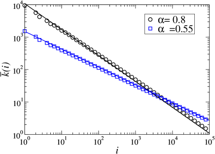
Figure 1: Average degree of the vertices with index $i$ in the original SM, for two different values of $\alpha$. The solid lines represent the theoretical value given by Eq. (27).

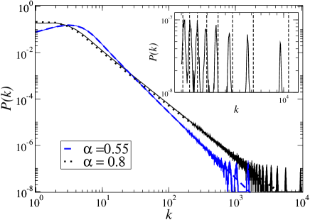
Figure 2: Degree distribution in the SM for two different values of $\alpha$. The dotted and dashed lines represent the theoretical value given by Eq. (35). In the inset: enlargement of the tail of the distribution. Peaks due to the discretization of the degree are visible. Dashed vertical lines represent the theoretical values of the centers of such peaks.

In Fig. 1 we plot the average degree of the vertices with index $i$, $\bar{k}(i)$ for two different values of $\alpha$, namely $\alpha=0.55$ and $\alpha=0.8$, which correspond to the degree exponents $\gamma=2.82$ and $\gamma=2.25$, respectively. In both cases, the analytical result, as as given by Eq. (27), fit almost perfectly the curves emerging from numerical simulation. The same happens for the degree distribution, shown in Fig. 2, for the two values of $\alpha$ considered. As we can see from this Figure, the complete expression calculated in Eq. (35) fits exactly the whole distribution, except at very large values of $k$. This discrepancy, due to the finite size of the networks, is easy to understand. From Eq.(27), we can observe that large values of $k$ correspond to small values of the index $i$. In this region, the continuous $i$ and $k$ approximation made in all calculations is expected to fail, and the index $i$ to show its true discrete nature. Indeed, this fact can be clearly observed in the inset in Fig. 2, where we plot a close-up of the tail of the degree distribution obtained for $\alpha=0.8$, obtained from averaging over $10^{3}$ network samples. This plot shows a set of peaks, corresponding to the first values of the index $i$, from $1$ to $8$. The centers of the peaks are well approximated by the analytical $\bar{k}(i)$ function given in Eq. (27), and represented by means of vertical dotted lines, except for very small values of $i$. The width of the peaks is accounted for by the fluctuations in the value of $k$ in the different network samples.

In Fig. 3 we report the average nearest neighbors degree of the vertices with index $i$. The dashed line represents the theoretical approximation obtained in Eq. (38). We find a percentually small difference between calculation and simulation. This difference can be attributed to the effect of the continuous approximation. Indeed, if we numerically calculate the sum of Eq. (37) and report it in the plot (continuous line), we obtain a better fit of the simulation results. A good agreement between theory and simulation is obtained as well in the plot of the average nearest neighbor degree of the vertices with degree $k$, Fig. 4, at least for sufficiently large values of $\alpha$. Here theoretical value is obtained directly from numerical summation of Eq. (39), that cannot be approximated analytically in a simple way. The correlation function displays an almost constant behavior at low degrees and a decreasing slope at high degrees, i.e. a regime without any correlation followed by one characterized by strong disassortative mixing. The emergence of these correlation is connected to the absence of multiple and self-connections. By doing this, we bias the natural tendency of high degree vertices to have some connections into each other, favoring their linking to small degree vertices, and, therefore, generating negative correlations in the degree. This phenomenon appears to be extremely relevant for small values of $\gamma$. In the case $\alpha=0.8$, for example, we can observe in the average neighbor connectivity a decay of more than one decade in about two decades of the degree. On the other hand, the analytical solutions does not behave so well for large values of $\gamma$ (small $\alpha$), probably due to the accumulated effect of all the approximations made in obtaining this expression.

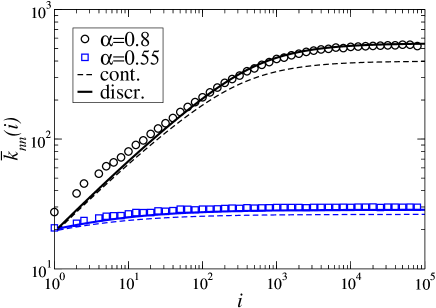
Figure 3: Average nearest neighbor degree of the vertices with index $i$ in the SM for two different values of $\alpha$. The solid lines represent the theoretical value given by the numerical summation of Eq. (37). The dashed lines correspond to the analytical approximation in the Eq. (38).

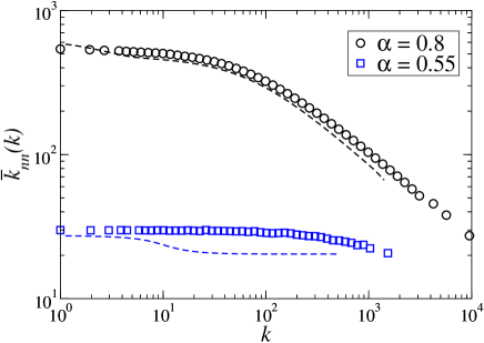
Figure 4: Average nearest neighbor degree of the vertices with degree $k$, in the SM for two different values of $\alpha$. The dashed lines correspond to the numerical summation of Eq. (39).

6 Conclusions

In this work we have presented an analytic solution of the static model static , which has been recently proposed as a paradigmatic scale-free non-growing network model. The solution is obtained via a mapping of the SM into a hidden variables network model, that represents its canonical counterpart, i.e. in which the number of edges is not held fixed, but whose average degree tends to a constant in the infinite network size limit. We have derived analytically the properties of the mapped hidden variables network model and checked the predictions by means of extensive numerical simulations of the original model. The good agreement observed implies that the canonical version of the SM is identical to the original version in the thermodynamic limit $N\to\infty$. It is particularly noteworthy that our analytical calculations have allowed us to evaluate the correlations induced in the model by the physical condition of absence of self and multiple connections. The detected amount of correlation is considerable and can have a strong influence both on the topology of the networks, and on dynamics running on top of them. The presence of these correlations thus casts some shadows on the usefulness of the SM as a benchmark for mean-field solutions of dynamical processes, which are usually obtained in the uncorrelated limit. In this sense, the recently proposed Uncorrelated Configuration Model ucm appears to be a more adequate instrument for the investigation of the effects of scale-invariance in network topology and dynamics, without the perturbations induced by the presence of correlations.

- (1) R. Pastor-Satorras and A. Vespignani, Evolution and structure of the Internet: A statistical physics approach (Cambridge University Press, Cambridge, 2004).
- (2) B. A. Huberman, The laws of the Web (MIT press, Cambridge, MA, USA, 2001).
- (3) M. E. J. Newman, Phys. Rev. E 64, 016131 (2001).
- (4) A.-L. Barabási, H. Jeong, Z. Néda, E. Ravasz, A. Schubert and T. Vicsek Physica A 311, 590 (2002).
- (5) F. Liljeros, C. R. Edling, L. A. N. Amaral, H. E. Stanley, and Y. Aberg, Nature 411, 907 (2001).
- (6) J. M. Montoya and R. V. Solé, J. Theor. Biol. 214, 405 (2002).
- (7) D. Garlaschelli, G. Caldarelli, and L. Pietronero, Nature 423, 165 (2003).
- (8) A. Wagner, Mol. Biol. Evol. 18, 1283 (2001).
- (9) H. Jeong, B. Tombor, R. Albert, Z. N. Oltvai, and A.-L. Barabási, Nature 407, 651 (2000).
- (10) B. Bollobás, Modern Graph Theory (Springer-Verlag, New York, 1998).
- (11) R. Albert and A.-L. Barabási, Rev. Mod. Phys. 74, 47 (2002).
- (12) S. N. Dorogovtsev and J. F. F. Mendes, Evolution of networks: From biological nets to the Internet and WWW (Oxford University Press, Oxford, 2003).
- (13) A.-L. Barabási and R. Albert, Science 286, 509 (1999).
- (14) R. A. Albert, H. Jeong, and A.-L. Barabási, Nature (London) 406, 378 (2000).
- (15) D. S. Callaway, M. E. J. Newman, S. H. Strogatz, and D. J. Watts, Phys. Rev. Lett. 85, 5468 (2000).
- (16) R. Cohen, K. Erez, D. ben Avraham, and S. Havlin, Phys. Rev. Lett. 86, 3682 (2001).
- (17) R. Pastor-Satorras and A. Vespignani, Phys. Rev. Lett. 86, 3200 (2001).
- (18) A. L. Lloyd and R. M. May, Science 292, 1316 (2001).
- (19) R. Pastor-Satorras, A. Vázquez, and A. Vespignani, Phys. Rev. Lett. 87, 258701 (2001).
- (20) M. Boguñá, R. Pastor-Satorras, Phys. Rev. E 68, 036112 (2003).
- (21) M. E. J. Newman, Phys. Rev. Lett. 89, 208701 (2002).
- (22) M. Catanzaro, G. Caldarelli, and L. Pietronero, Phys. A 338, 119-124 (2004).
- (23) G. Caldarelli, A. Capocci, P. De Los Rios, and M. A. Muñoz, Phys. Rev. Lett. 89, 258702 (2002).
- (24) B. Söderberg, Phys. Rev. E 66, 066121 (2002).
- (25) K.-I. Goh, B. Kahng, and D. Kim, Phys. Rev. Lett. 87, 270701 (2001).
- (26) M. Barthélemy, Phys. Rev. Lett. 91, 189803 (2003).
- (27) M. Barthélemy, Eur. Phys. J. B 38, 163-168 (2004).
- (28) K.-I. Goh, D.-S. Lee, B. Kahng, and D. Kim, Phys. Rev. Lett. 91, 148701 (2003).
- (29) D. S. Lee, cond-mat/0410635.
- (30) S. N. Dorogovtsev and J. F. F. Mendes, Adv. Phys. 51, 1079 (2002).
- (31) M. Boguñá, R. Pastor-Satorras, and A. Vespignani, Euro. Phys. J. B 38, 205 (2004).
- (32) P. Erdös and P. Rényi, Publicationes Mathematicae 6, 290 (1959).
- (33) M. Abramowitz and I. A. Stegun, Handbook of mathematical functions. (Dover, New York, 1972).
- (34) P. Bratley, B. L. Fox, and L. E. Schrage A guide to simulation. Second edition. (Springler-Verlag, New York, 1987).
- (35) M. Catanzaro, M. Boguñá, and R. Pastor-Satorras, cond-mat/0408110.