Abstract

The Boltzmann entropy $S^{(B)}$ is true in the case of equal probability of all microstates of a system. In the opposite case it should be averaged over all microstates that gives rise to the Boltzmann–Shannon entropy (BSE). Maximum entropy principle (MEP) for the BSE leads to the Gibbs canonical distribution that is incompatible with power–low distributions typical for complex system. This brings up the question: Does the maximum of BSE correspond to an equilibrium (or steady) state of the complex system? Indeed, the equilibrium state of a thermodynamic system which exchange heat with a thermostat corresponds to maximum of Helmholtz free energy rather than to maximum of average energy, that is internal energy $U$. Following derivation of Helmholtz free energy the Renyi entropy is derived as a cumulant average of the Boltzmann entropy for systems which exchange an entropy with the thermostat. The application of MEP to the Renyi entropy gives rise to the Renyi distribution for an isolated system. It is investigated for a particular case of a power–law Hamiltonian. Both Lagrange parameters, $\alpha$ and $\beta$ can be eliminated. It is found that $\beta$ does not depend on a Renyi parameter $q$ and can be expressed in terms of an exponent $\kappa$ of the power–law Hamiltonian and $U$. The Renyi entropy for the resulting Renyi distribution reaches its maximal value at $q=1/(1+\kappa)$ that can be considered as the most probable value of $q$ when we have no additional information on behavior of the stochastic process. The Renyi distribution for such $q$ becomes a power–law distribution with the exponent $-(\kappa+1)$. Such a picture corresponds to some observed phenomena in complex systems.

KEY WORDS: Stability condition, Helmholtz free energy, Renyi entropy, Tsallis entropy, escort distribution, power–law distribution.

1 Introduction

The well–known Boltzmann formula defines a statistical entropy, as a logarithm of number of states $W$ attainable for the system

$$S^{(B)}=\ln W$$ (1)

Here and below the entropy is written as dimensionless value without the Boltzmann constant $k_{B}$.

This definition is valid not only for physical systems but for much more wide class of social, biological, communication and other systems described with the use of statistical approach. The only but decisive restriction on the validity of this equation is the condition that all $W$ states of the system have equal probabilities (such systems are described in statistical physics by a microcanonical ensemble). It means that probabilities $p_{i}=p_{W}=1/W$ (for all $i=1,2,...,W$) that permits to rewrite the Boltzmann formula (1) as

$$S^{(B)}=-\ln p_{W}.$$ (2)

When the probabilities $p_{i}$ are not equal we can introduce an ensemble of microcanonical subsystems in such a manner that all $W_{i}$ states of the $i$-th subsystem have equal probabilities $p_{i}$ and its Boltzmann entropy is $S_{i}^{(B)}=-\ln p_{i}$. The simple averaging of the Boltzmann entropy $S_{i}^{(B)}$ leads to the Gibbs–Shannon entropy

$$S^{(G)}=\langle S_{i}^{(B)}\rangle_{p}\equiv-\sum_{i}p_{i}\ln p_{i}.$$ (3)

Just such derivation of $S^{(G)}$ is used in some textbooks (see, e. g. [1, 2]). This entropy is generally accepted in statistical thermodynamics and conventional in a communication theory.

According to maximum information principle (MEP) developed by Jaynes [3] for a Gibbs–Shannon statistics an equilibrium distribution of probabilities $p=\{p_{i}\}$ must provide maximum of the Gibbs–Shannon information entropy $S^{(B)}(p)=-k_{B}\sum_{i}\,p_{i}\ln p_{i}$ upon additional conditions of normalization $\sum_{i}p_{i}=1$ and a fixed average energy

$$U=\langle H\rangle_{p}\equiv\sum_{i}H_{i}p_{i},$$ (4)

where $H=\sum_{i}H_{i}$ is the Hamiltonian of the system.

Then, the distribution $\{p_{i}\}$ is determined from the extremum of the functional

$$L_{G}(p)=-\sum_{i}^{W}\,p_{i}\ln p_{i}-\alpha_{0}\sum_{i}^{W}\,p_{i}-\beta_{0}\,\sum_{i}^{W}H_{i}p_{i},$$ (5)

where $\alpha_{0}$ and $\beta_{0}$ are the Lagrange multipliers. Its extremum is ensured by the Gibbs canonical distribution

$$p^{(G)}_{i}=Z_{G}^{-1}e^{-\beta_{0}H_{i}},$$ (6)

in which $\beta_{0}$ is determined by condition of correspondence between Gibbs thermostatistics and classical thermodynamics as $\beta_{0}=1/k_{B}T_{0}$where $T_{0}$is the thermodynamic temperature.

However, when investigating complex physical systems (for example, fractal and self-organizing structures, turbulence) and a variety of social and biological systems, it appears that the Gibbs distribution does not correspond to observable phenomena. In particular, it is not compatible with a power-law distribution that is typical [4] for such systems. Introducing of additional restrictions to a sought distribution in the form of conditions of true average values $\langle X^{(m)}\rangle_{p}$ of some physical parameters of the system $X^{(m)}$ gives rise to a generalized Gibbs distribution with additional terms in the exponent (6) but does not change its exponential form.

2 Helmholtz free energy and Renyi entropy

There is no doubts about the MEP as itself, because of it is a kind of "a maximum honesty principle" according to which we demand a maximal uncertainty from the distribution apart from true description of prescribed averages. In the opposite case we risk to introduce a false information into the description of the system.

Thus, it only remains for us to throw doubt on the information entropy form. To seek out a direction of modification of the Gibbs–Shannon entropy we consider first extremal properties of an equilibrium state in thermodynamics.

A direct calculation of the average energy of a system gives the internal energy (4), its extremum is characteristic of an equilibrium state of rest for a mechanical system, other than a thermodynamic system that can change heat with a thermostat. An equilibrium state of the latter system is characterized by extremum of the Helmholtz free energy $F$. To derive it statistically from the Hamiltonian without use of thermodynamics we introduce generating function [5]introduce generating function for the random value $H=-\sum_{i}H_{i}$

$$\Phi_{H}(\lambda)=\sum_{i}e^{\lambda H_{i}},$$ (7)

where $\lambda$ is the arbitrary constant, and construct a cumulant generating function

$$\Psi_{H}(\lambda)=\ln\Phi_{H}(\lambda)$$ (8)

that becomes the Helmholtz free energy $F$ when devided by $\lambda$ that is chosen as $\lambda=-1/k_{B}T_{0}$.

Now we return to the problem of a generalized entropy for open complex systems. Exchange by both energy and entropy is characteristic for them. As an illustration, there is a description by Kadomtsev [6] of self-organized structure in a plasma sphere: "The entropy is being born continuously within the sphere and flowing out into surroundings. If the entropy flow had been blocked, the plasma would ’die’. It is necessary to remove continuously ’slag’ of newly produced entropy".

That is the reason why the Gibbs–Shannon entropy, derived by the simple averaging of the Boltzmann entropy can not be function of which extremum characterizes a steady state of a complex system which exchange entropy with surroundings, just as the minimum of the internal energy does not characterize an equilibrium state of the thermodynamic system being in heat contact with a heat bath.

An effort may be made to find a "free entropy" of a sort by the same way that was used above for derivation of the Helmholtz free energy. The generating function is introduced as

$$\Phi_{S}(\lambda)=\sum_{i}e^{\lambda S_{i}^{(B)}}$$ (9)

Then the cumulant generating function is

$$\Psi_{S}(\lambda)=\ln\Phi_{S}(\lambda)=\ln\sum_{i}p_{i}^{-\lambda}.$$ (10)

To obtain the desired generalization of the entropy we are to find a $\lambda$-dependent numerical coefficient which ensures a limiting pass of the new entropy into the Gibbs–Shannon entropy. Such the coefficient is $(\lambda+1)$. Indeed, the new $\lambda$-family of entropies

$$S(\lambda)=\frac{1}{1+\lambda}\ln\sum_{i}p_{i}^{-\lambda}.$$ (11)

includes the Gibbs–Shannon entropy as a particular case when $\lambda\to-1$.

Thus, it has appeared that the desired "free entropy" coincides with the known Renyi entropy [7]. It is conventional to write it with the parameter $q=-\lambda$ in the form

$$S^{(R)}(p)=\frac{1}{1-q}\ln\sum_{i}p_{i}^{q}$$ (12)

The same result can be obtained with the use of a Kolmogorov–Nagumo [8, 9] generalized averages of the form

$$\langle x\rangle_{\phi}=\phi^{-1}\left(\sum_{i}p_{i}\phi(x_{i})\right)$$ (13)

where $\phi(x)$ is an arbitrary continuous and strictly monotonic function and $\phi^{-1}(x)$ is the inverse function. It had been just this kind of average that was used by Renyi [10] to define his new entropy as a generalized average of the Boltzmann entropy (1). As a result of choice of the Kolmogorov–Nagumo function in the form $\phi(x)=e^{(1-q)x}$ he obtained (12). Such the choice of $\phi(x)$ appears accidental until it is not pointed that the same exponential function of the Hamiltonian provides derivation of the free energy that is extremal at an equilibrium state of a thermodynamic system which exchange heat with a heat bath. This fact permits to suppose that the Renyi entropy derived in the same manner is extremal at a steady state of a complex system which exchange entropy with its surroundings very actively.

Different properties of the Renyi entropy are discussed in particular in Refs. [7, 11, 12]. It is positive ($S^{(R)}\geq 0$), convex at $q\leq 1$, passes into the Gibbs–Shannon entropy $\lim_{q\rightarrow 1}S^{(R)}=S^{G}$ and into Boltzmann entropy (1) for any $q$ in the case of equally probable distribution $p$.

In the case of $|1-\sum_{i}p_{i}^{q}|\ll 1$ (which, in view of normalization of the distribution $\{p_{i}\}$, corresponds to the condition $|1-q|\ll 1$), one can restrict oneself to the linear term of logarithm expansion in the expression for $S^{(R)}(p)$ over this difference, and $S^{(R)}(p)$ changes to the Tsallis entropy [13]

$$S^{(T)}(p)=-\frac{k_{B}}{1-q}(1-\sum_{i}^{W}p_{i}^{q}).$$ (14)

The logarithm linearization results in the entropy becoming nonextensive, that is, $S(W_{1}W_{2})\neq S(W_{1})S(W_{2})$. This property is widely used by Tsallis and by the international scientific school that has developed around him for the investigation of diverse nonextensive systems (see web site [14]). In so doing, the above-identified restriction $|1-q|\ll 1$ is disregarded. As a result of nonextensivity the Tsallis entropy incompatible with the Boltzmann entropy (1) because of the latter was derived by Plank in such the form just from the extensivity condition $S(W_{1}W_{2})=S(W_{1})S(W_{2})$.

3 MEP for Renyi entropy

If the Renyi entropy is used in MEP instead of the Gibbs–Shannon entropy, the equilibrium distribution is to be looked for from the maximum of the functional

$$L_{R}(p)=\frac{1}{1-q}\,\ln\sum_{i}^{W}\,p^{q}_{i}-\alpha\sum_{i}^{W}\,p_{i}-\beta\,\sum_{i}^{W}H_{i}p_{i},$$ (15)

where $\alpha$ and $\beta$ are Lagrange multipliers. It can be noticed that $L_{R}(p)$ passes to $L_{G}(p)$ in the $q\to 1$ limit.

We equate a functional derivative of $L_{R}(p)$ to zero, then

$$\frac{\delta L_{R}(p)}{\delta p_{i}}=\frac{q}{1-q}\,\frac{p_{i}^{q-1}}{\sum_{j}p_{j}^{q}}-\alpha-\beta H_{i}=0.$$ (16)

To eliminate the parameter $\alpha$ we can multiply this equation by $p_{i}$ and sum up over $i$, taking into account the normalization condition $\sum_{i}p_{i}=1$. Then we get

$$\alpha=\frac{q}{1-q}-\beta U$$ (17)

and

$$p_{i}=\left((1-\beta\frac{q-1}{q}\Delta H_{i})\,\sum_{j}^{W}\,p^{q}_{j}\right)^{\frac{1}{q-1}},\,\,\Delta H_{i}=H_{i}-U.$$ (18)

Using once more the condition $\sum_{i}p_{i}=1$ we get

$$\sum_{j}^{W}\,p_{j}^{q}=\left(\sum_{i}^{W}(1-\beta\frac{q-1}{q}\Delta H_{i})^{\frac{1}{q-1}}\right)^{-(q-1)}$$

and, finally, we get [15, 16] the Renyi distribution

$$p_{i}=p_{i}^{(R)} = Z_{R}^{-1}\left(1-\beta\frac{q-1}{q}\Delta H_{i}\right)^{\frac{1}{q-1}}$$ (19)

$$Z_{R}^{-1} = \sum_{i}\left(1-\beta\frac{q-1}{q}\Delta H_{i}\right)^{\frac{1}{q-1}}.$$ (20)

When applying MEP to the Tsallis entropy it is necessary to take into account that all average values in the last version of nonextensive thermostatistics [17] are calculated with the use of an escort distribution $P_{i}=p_{i}^{q}/\sum_{i}p_{i}^{q}$ that contradicts to the main principles of probability description. Indeed, at $q>1$ ($q<1$), the importance of $p_{i}$ with the maximal (minimal) values increases. In view of this, it is evident that use of the escort distribution in statistical thermodynamics does not lead to true average values of dynamical variables. Nevertheless, the additional condition of a fixed mean energy in nonextensive thermostatistics is written as $U=\langle H\rangle_{es}\equiv\sum_{i}H_{i}\,P_{i}$ and the escort Tsallis distribution is found in the form

$$P_{i}^{(Ts)}=Z_{Ts}^{-1}\left(1-\beta^{*}(1-q^{\prime})\Delta H_{i}\right)^{\frac{q^{\prime}}{1-q^{\prime}}}\\$$ (21)

where $\beta^{*}=\beta/\sum_{i}p_{i}^{q}$ and $\beta$ is the Lagrange multiplier.

It should be noticed that both Renyi and escort Tsallis distributions, Eqs. (19) and (21), are identical if $q^{\prime}=1/q$. In reality, in this case

$$1-q^{\prime}=\frac{q-1}{q},\,\,\,\,\,\frac{q^{\prime}}{1-q^{\prime}}=\frac{1}{q-1}$$ (22)

and $\beta^{*}$ is determined by the same second additional condition (4) of MEP as well as $\beta$.

Thus, not always justified linearization of the logarithm in the Renyi entropy and questionable use of the escort distribution leads to the same Renyi distribution if $q$ and $q^{\prime}$ are considered as free parameters.

Therefore, numerous works (see [14]) confirming correspondence of the Tsallis escort distribution (with fitted $q^{\prime}$) with distributions in complex physical, biological, social and other systems count rather in favor more justified Renyi entropy than nonextensive Tsallis entropy.

When $q\to 1$ the distribution $\{p^{(R)}_{i}\}$ becomes the Gibbs canonical distribution and $\beta/q\to\beta_{0}=1/k_{B}T_{0}$. Such behavior is not enough for unique determination of $\beta$, as in general, it may be an arbitrary function $\beta(q)$ which becomes $\beta_{0}$ in the limit $q\to 1$.

To find an explicit form of $\beta$, we return to the additional condition of the pre-assigned average energy and substitute there the Renyi distribution (19). Then we obtain the integral equation for $\beta$

$$U=\sum^{W}_{i}H_{i}p^{(R)}_{i},$$ (23)

where $U$ is considered as a known value. This equation was solved [16] for a particular case of a power-law dependence of the Hamiltonian on a parameter $x$

$$H_{i}=Cx_{i}^{\kappa}.$$ (24)

This type of the Hamiltonian corresponds to an ideal gas model in the Boltzmann-Gibbs thermostatistics and it seems reasonable to say that it may be useful in construction of thermostatistics of complex systems. Moreover, in most social, biological and humanitarian sciences the system variable $x$ can be considered (with $\kappa=1$) as a kind of the Hamiltonian (e.g. the size of population of a country, effort of a word pronouncing and understanding, bank capital, number of scientific publications of an author, size of an animal etc.).

For the power-law Hamiltonian the convergence condition for the sum in Eq. (23) in the limiting case $W\to\infty$ is

$$q>q_{min}=1/(1+\kappa)$$ (25)

As a result of solution of equation (23) the parameter $\beta$ is found as

$$\beta=\frac{1}{\kappa U}$$ (26)

Independence of this relation from $q$ means that it is true, in particular, for the limit case $q=1$ where the Gibbs distribution takes a place and, therefore,

$$\beta=\beta_{0}\equiv 1/k_{B}T\,\,\,\,{\rm for\,\,all}\,\,q.$$ (27)

When $H=p^{2}/2m$ (that is, $\kappa=2$) we get from (26) and (27) that $U=\frac{1}{2}k_{B}T_{0}$, as would be expected for one-dimensional ideal gas.

The Lagrange parameter $\beta$ can be eliminated from the Renyi distribution (19) with the use of Eq. (26) and we have, alternatively,

$$p^{(R)}_{i}=Z^{-1}\left(1-\frac{q-1}{\kappa q}(C_{u}x^{\kappa}_{i}-1)\right)^{\frac{1}{q-1}},\,\,\,H_{i}=Cx_{i}^{\kappa},\,\,\,C_{u}=C/U.$$ (28)

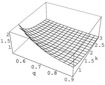
Figure 1: The entropies $S^{(R)}[p^{(R)}(q,\kappa)]$ (top) and $S^{(B)}[p^{(R)}(q,\kappa)]$ (bottom) for the power–law Hamiltonian with the exponent $\kappa$ within the range $3>\kappa>0.5$ and $q>1/(1+\kappa)$.

The problem to be solved for a unique definition of the Renyi distribution is determination of a value of the Renyi parameter $q$. This will be the subject of the next section.

4 The most probable value of the Renyi parameter

An excellent example of solution of this problem for a physical non-Gibbsian system was presented by Wilk and Wlodarczyk [18]. They took into consideration fluctuations of both energy and temperature of a minor part of a large equilibrium system. This is a radical difference of their approach from the traditional Gibbs method in which temperature is a constant value characterizing the thermostat. As a result, their approach led (see [19]) to the Renyi distribution with the parameter $q$ expressed via heat capacity $C_{V}$ of the minor subsystem

$$q=\frac{C_{V}-k_{B}}{C_{V}}.$$ (29)

The approach by Wilk and Wlodarczyk was advanced by Beck [20] and Beck and Cohen [21] who offered for it a new apt term "superstatistics". In the frame of superstatistics, the parameter $q$ is defined by physical properties of a system which can exchange energy and heat with a thermostat. As a result, $q\neq 1$ but $|q-1|\ll 1$, because of exchange entropy is not taken into account by superstatistics.

In general, when we have no information about nature of a stochastic process the parameter $q$ is considered as a free parameter. So, the proposed further extension of MEP consists in looking for a maximum of the Renyi entropy in a space of the Renyi distributions with different values of $q$.

In reality, maximum of the RE is ensured by the Renyi distribution function (28) for any fixed $q$ fulfilling the inequality (25). The next step consists of substitution of the Renyi distribution $p^{(R)}(q,\kappa)$ into the definition of the Renyi entropy, Eq. (13), and variation of the $q$-parameter. The resultant picture of $S^{(R)}[p^{(R)}(q,\kappa)]$ as a function of $q$ is illustrated in Fig. 1 (left). It is seen that $S^{(R)}[p^{(R)}(q,\kappa)]$ attains its maximum at the minimal possible value $q=q_{min}$. For $q<q_{min}$, the series (23) diverges and, therefore, the Renyi distribution does not determine the average value $U=\langle H\rangle_{p}$, that is a violation of the second condition of MEP.

The similar procedure is applied to the Gibbs-Shannon entropy $S^{(B)}(p)$, as well. Substituting there $p=p^{(R)}(q,\kappa)$ we get the $q$-dependent function $S^{(B)}[p^{(R)}(q,\kappa)]$ illustrated in Fig. 1 (right). As would be expected, the Gibbs-Shannon entropy $S^{(B)}[p^{(R)}(q,\kappa)]$ attains its maximum value at $q=1$ where $p^{(R)}(q,\kappa)$ becomes the Gibbs canonical distribution.

Thus, it is found that the maximum of the Renyi entropy is realized at $q=q_{min}$ and it is just the value of the Renyi parameter that should be used if we have no additional information on behavior of the stochastic process under consideration.

Recall that the Renyi entropy was derived above as a functional which attain its maximum value at the equilibrium state (or steady state) of a complex system just as the Helmholtz free energy for a thermodynamic system. (The kind of extremum, that is, maximum or minimum is determined by the sign definition for the constant $\lambda$.) Then, a radically important conclusion follows from comparision of these two graphs:

In contrast to the Gibbs–Shannon entropy the Renyi entropy increases as a system complexity (departure of the $q$ value from 1) increases that permits to explain an evolution of the system to self-organization from the point of view of thermodynamical stability.

It counts in favor of such the conclusion that a power–law distribution characteristic for self-organizing systems [4] is realized when the Renyi entropy is maximal. Substitution of $q=q_{min}$ into Eq. (28) does lead to

$$p=Z^{-1}x^{-(1+\kappa)}$$ (30)

Thus, for $q=q_{min}$ the Renyi distribution for a system with the power–law Hamiltonian becomes power–low distribution over the whole range of $x$.

For a particular case of the impact fragmentation where $H\sim m^{2/3}$ the power-law distribution of fragments over their masses $m$ follows from (21) as $p(m)\sim m^{-5/3}$ that coincides with results of our previous analysis [22] and experimental observations [23].

For another particular case, $\kappa=1$, power–low distribution is $p\sim x^{-2}$. Such a form of the Zipf-Pareto law is the most useful in social, biological and humanitarian sciences. The same exponent of power–low distribution was demonstrated [24] for energy spectra of particles from atmospheric cascades in cosmic ray physics and for distribution of users among the web sites [25].

I acknowledge fruitful discussions of the subject with A. V. Vityazev.

References

- [1] H. Haken. Information and Self-Organization. Berlin, Springer, 1988.
- [2] J. S. Nicolis. Dynamics of Hierarchial Systems. An Evolutionary Approach. Springer, Berlin, 1986.
- [3] E.T. Jaynes. Phys.Rev. 106:620; 107:171 (1957).
- [4] P. Bak How nature works: the science of self-organized criticality. N.-Y., Copernicus, 1996.
- [5] R. Balescu. Equilibrium and nonequilibrium statistical mechanics. N.-Y. John Wiley and Sons, Inc. 1975.
- [6] B. B. Kadomtsev. Dynamics and information. oscow, Published by Uspechi Fizicheskikh Nauk, 1997.
- [7] A. Renyi. Probability theory, North-Holland, Amsterdam (1970).
- [8] A. N. Kolmogorov. Atti R. Accad. Naz. Lincei 12:388 (1930).
- [9] M. Nagumo . Japan J. Math. 7:71 (1930).
- [10] Selected papers by Alfred Renyi, Vol. 2, Akademiai Kiado, Budapest, 1976.
- [11] C. Beck, F. Schlögl. Thermodynamics of Chaotic Systems, Cambridge Univ. Press, Cambridge (1993).
- [12] Yu.L. Klimontovich. Statistical Theory of Open Systems. Kluwer Academic Publishers. Dordrecht, 1994.
- [13] C. Tsallis. J.Stat.Phys. 52:479 (1988)
- [14] http://tsallis.cat.cbrf.br/biblio.htm
- [15] A.G. Bashkirov. Physica A 340:153-162 (2004).
- [16] A.G. Bashkirov. Phys. Rev. Lett. :N13, 13061 (2004).
- [17] C. Tsallis, R.S. Mendes and A.R. Plastino. Physica A 261:534 (1998).
- [18] G. Wilk and Z. Wlodarczyk. Phys. Rev. Lett. 84:2770 (2000).
- [19] A. G. Bashkirov and A. D. Sukhanov. Zh. Eksp. Teor. Fiz. 122:513 (2002) [JETP 95:440 (2002)].
- [20] C. Beck. Phys. Rev. Lett. 87:18601 (2001).
- [21] C. Beck and E.G.D. Cohen. Physica A 322:267 (2003).
- [22] A.G. Bashkirov and A.V. Vityazev. Planet. Space Sci. 44:909 (1996).
- [23] A. Fujiwara, G. Kamimoto and A. Tsukamoto. Icarus 31, 277 (1977)
- [24] M. Rybczyski, Z. Wlodarczyk and G. Wilk. Nucl. Phys. B (Proc. Suppl.) 97:81 (2001).
- [25] L. A. Adamic and B. A. Hubermann. Glottometrics 3:143 (2002).