Energy barrier for collapse in a pair of tunnel-coupled condensates with the scattering lengths of opposite signs

Abstract

We predict the existence of an energy barrier for collapse in a system of two tunnel-coupled repulsive and attractive quasi two-dimensional condensates trapped in a double-well potential. The ground state in such a system can have a lower energy than that of the collapsing state. We find such ground states numerically and analytically determine the domain of their existence, they have a much larger share of atoms confined in the repulsive condensate. The energy barrier for collapse is due to the fact that the energy of the system increases if atoms tunnel from the repulsive condensate to the attractive one.

I Introduction

Bose-Einstein condensates (BEC) of degenerate quantum gases at zero temperature are described with a good accuracy by the mean-field theory based on the nonlinear Schrödinger equation with an external potential, i.e., the well-known Gross-Pitaevskii (GP) equation GPE for the order parameter. The appearance of the order parameter is a consequence of the macroscopic quantum coherence of BEC, which was demonstrated experimentally intrfexp ; intrf2comp and explained theoretically intrfth with the use of the GP equation (see also the review Ref. BECRev ).

The interplay between the quantum coherence and nonlinearity in BEC is a reach source of interesting new phenomena. In this paper we predict such a new phenomenon related to the collapse instability of an attractive BEC. The collapse in the condensate with a negative scattering length is extensively studied experimentally and theoretically (see, for instance, Refs. addCollapse ; expCollapseBEC ; expCollapseBEC2 ; theorCollapseBEC ; CollapseBEC ; ComparTheorExpCollapse and the references therein). The multi-component (multi-species) BECs were also shown to suffer from the collapse instability multCollapse1 ; multCollapse2 ; multCollapse3 ; multCollapse4 . Collapse of a repulsive BEC can be induced by a sudden change of its positive scattering length to a negative value by application of the magnetic field near the Feshbach resonance Fesh ; Fesh2D . Here we show that with the use of a coherent coupling between two BECs with the opposite interactions (one repulsive and the other attractive) it is possible to modify significantly the properties of the collapse instability. An experimental realization is provided by a pair of condensates trapped in the double-well potential with far separated wells, when the atomic scattering length changes sign in just one of the condensates. The coherent coupling is achieved by the quantum tunnelling through the central barrier of the double-well trap.

There are two general geometric limits for the condensates trapped in a double-well potential: the one- and two-dimensional cases. In the one-dimensional case the condensates assume the cigar shaped form, while in the two-dimensional case they have the form of a pancake. We consider the two-dimensional case and rely on the important fact that the quasi two-dimensional Feshbach resonance is possible Fesh2D . The one-dimensional nonlinear Schrödinger equation describing the cigar shaped condensate has no collapsing solutions, they appear only when the transverse degrees of freedom are taken into account.

The stationary states in a pair of tunnel-coupled BECs bifurcate from the zero solution. In this limit the two condensates with opposite interactions can be described by a single effective equation of the nonlinear Schrödinger type with the nonlinearity being repulsive or attractive depending on the parameters. When the effective interaction is repulsive the system is stable, whereas, under certain condition on the number of atoms, the attractive effective interaction causes collapse.

The surprising fact is, however, that the ground state in a pair of tunnel-coupled repulsive and attractive condensates can have a lower energy than the stationary state unstable with respect to collapse. Therefore, for some values of the parameters, there is an energy barrier for collapse in the system. Recall that in a single nonlinear Schrödinger equation it is, in fact, the ground state which suffers from the collapse instability theorCollapseBEC ; CollapseBEC ; ComparTheorExpCollapse .

This work is related to our previous study Nova of the tunnel-coupled condensates in two spatial dimensions, where we have considered the stationary states of the system but without analysis of the ground state. Here we focus on the analysis of the ground state in the system and its energy, whereas the detailed derivation of the coupled-mode system and some of the auxiliary analytical results can be found in our previous publications Refs. Nova ; DW1D ; PhysD .

The paper is organized as follows. Section II contains analysis of the ground states in the system in the coupled-mode approximation, i.e. for far separated wells of the double-well trap. We conclude with the summary of the results in section III. The details of the linear stability analysis of the stationary solutions are relegated to the Appendix.

II Stationary states in the coupled-mode approach

Experimental realization of the scattering length management in just one of the two condensates trapped in a double-well potential necessitates that the wells be far separated. The lower two energy levels in such a double-well potential are quasi-degenerate and there is a large energy gap separating them from the rest of the energy spectrum. An ideal quantum gas in such a trap would occupy the degenerate subspace. For the condensate of an interacting gas there is a localized basis in the degenerate subspace which allows one to reduce the three-dimensional Gross-Pitaevskii equation to a system of linearly coupled two-dimensional equations (see also Ref. DW1D ). Indeed, due to the localization of the basis wave functions in the different wells of the double-well trap, the nonlinear cross-terms describing the atomic interaction between the two condensates are negligible.

The central barrier in the double-well trap can be created by a laser modulation of the parabolic potential. Assuming that the parabolic trap allows for the pancake shaped condensates, i.e. that the trap frequencies satisfy $\gamma=\omega_{z}/\omega_{\perp}\gg 1$, we can separate the spatial degrees of freedom, that is the order parameter for each of the two condensates factorizes: $\Psi(x,y,z,t)=\Phi_{\perp}(x,y,t)\psi_{\parallel}(z)$, with $\psi_{\parallel}(z)$ being one of the wave functions of the localized basis. By the above factorization we neglect the nonlinear term in the Gross-Pitaevskii equation as compared to the kinetic term along the double-well trap, i.e. we assume

$$\frac{\hbar^{2}}{2m}\frac{1}{\ell_{z}^{2}}\gg|g||\Psi|^{2},$$ (1)

where $\ell_{z}$ is an estimate of the condensate length in the $z$-direction and $g=4\pi a_{s}/m$ is the nonlinear coefficient in the Gross-Pitaevskii equation GPE . The longitudinal kinetic term is compensated by the external potential, hence $\ell_{z}=\sqrt{{\hbar}/(m\omega_{z})}$.

The Hamiltonian of an atom in the double-well trap can be put in the form DW1D ; Nova

$$H=\mathcal{E}|R\rangle\langle R|-K(|R\rangle\langle L|+|L\rangle\langle R|),$$ (2)

where $|L\rangle$ and $|R\rangle$ are the localized basis, $\mathcal{E}$ can be identified with the zero-point energy difference and $K$ with the tunnelling coefficient. Under the condition (1) supplemented by the assumption of far separated wells of the trap and the quasi degeneracy of the energy levels, i.e. $K\ll\hbar\omega_{z}$ and $\mathcal{E}\ll\hbar\omega_{z}$, the Gross-Pitaevskii equation reduces to the coupled-mode system describing evolution of the condensates in the transverse dimensions:

$$i\partial_{T}u = \left(-\nabla^{2}+\vec{\rho}\,{}^{2}\right)u-|u|^{2}u-\kappa v,$$ (3a)

$$i\partial_{T}v = \left(-\nabla^{2}+\vec{\rho}\,{}^{2}\right)v+(\varepsilon+a|v|^{2})v-\kappa u$$ (3b)

(see also Ref. Nova ). We have used the dimensionless variables: $T=\omega_{\perp}t/2$ and $\vec{\rho}={\vec{r}}/{\ell_{\perp}}$ (the coordinate in the transverse plane), with $\ell_{\perp}=\sqrt{{\hbar}/(m\omega_{\perp})}$. Here $\kappa=2K/(\hbar\omega_{\perp})$, $\varepsilon=2{\mathcal{E}}/(\hbar\omega_{\perp})$, and $a=a^{(v)}_{s}/|a^{(u)}_{s}|$ is the relative scattering coefficient (we assume that $a^{(u)}_{s}<0$ and $a^{(v)}_{s}>0$). The term $\rho^{2}$ in the system (3) is due to the common transverse parabolic trap. Note that due to $\gamma\gg 1$ the coefficients $\kappa$ and $\varepsilon$ are not small in general.

The transverse order parameters for the two condensates can be expressed as $\Phi_{u}=(\sqrt{\Delta}/\ell_{\perp})u$ and $\Phi_{v}=(\sqrt{\Delta}/\ell_{\perp})v$, with $\Delta=(8\pi|a^{(u)}_{s}|\int\mathrm{d}z|\psi_{\parallel}|^{4})^{-1}$ Nova . For the current experimental traps the parameter $\Delta$ is on the order of $10^{2}-10^{3}$. In the numerics below we use the quantities $N_{u}=\int\mathrm{d}^{2}\vec{\rho}\,|u|^{2}$ and $N_{v}=\int\mathrm{d}^{2}\vec{\rho}\,|v|^{2}$ referring to them as the number of atoms, for short, though the actual number of atoms is larger by the factor $\Delta$. Finally, the condition (1) in the dimensionless form reads:

$$N_{u}\ll\gamma R_{u}^{2},\quad aN_{v}\ll\gamma R_{v}^{2},$$ (4)

where $R_{u}$ and $R_{v}$ are the radii of the two condensates measured in the units of $\ell_{\perp}$.

The stationary states with the chemical potential $\mu$ are sought in the form $u=e^{-i\mu T}U(\rho)$ and $v=e^{-i\mu T}V(\rho)$. In general, there are two types of the real solutions $U$ and $V$, satisfying the inequalities $UV>0$ (positive) and $UV<0$ (non-positive). The positive stationary states bifurcate from zero at $\mu=\mu_{\mathrm{bif}}$, where $\mu_{\mathrm{bif}}=2+\varepsilon/2-\sqrt{\varepsilon^{2}/4+\kappa^{2}}$, while the non-positive ones at $\mu_{\mathrm{bif}}^{\prime}=2+\varepsilon/2+\sqrt{\varepsilon^{2}/4+\kappa^{2}}$. The bifurcation points are easily found by analysis of the linear part of the stationary coupled-mode system which follows from the system (3) for the vanishing amplitude solutions $U$ and $V$, given as $U=Ae^{-\rho^{2}/2}$ and $V=Be^{-\rho^{2}/2}$ with $B=(2-\mu)A/\kappa$ and $A\to 0$. Being interested in the ground state of the system, we need to consider only the positive solutions since they bifurcate from the zero solution at a lower energy. Below the stationary solution (state) means the positive solution.

The stationary states were found by using the numerical approach of Ref. PhysD , i.e. by iterative solution in the polar coordinates of the nonlinear eigenvalue problem arising from the system (3) (with $\mu$ being the nonlinear eigenvalue). Our method allows for the simultaneous computation of the stationary state and the chemical potential $\mu$, with the same accuracy. We have used the Fourier pseudo-spectral method with the spatial grid containing 256 grid points.

We have found that the sufficient condition for stability of the stationary state of the system (3) is given by the Vakhitov-Kolokolov (VK) criterion: $\partial N/\partial\mu<0$, with $N=N_{u}+N_{v}$ being the total number of atoms. Moreover, if the effective interaction is repulsive (see below) then the ground state solution is unconditionally stable. The applicability of the VK criterion for stability in the case of the two-dimensional coupled-mode system is partially based on the numerical analysis of the appropriate eigenvalue problems, as discussed in the Appendix.

If the tunnel-coupling were absent ($\kappa=0$) the attractive $u$-condensate would collapse for $N_{u}>N_{\mathrm{th}}\approx 11.69$. This threshold for collapse in the parabolic trap is given by the number of atoms in the so-called Townes soliton (see, for instance, Ref. Collapse2D ). We have found that in the system (3) with $a\geq 0$ the stationary states unstable with respect to collapse always appear in the limit of large negative $\mu$ and have $N\to N_{\mathrm{th}}$ as $\mu\to-\infty$. For some values of the system parameters the collapsing states exist for finite negative values of $\mu$ (see Fig. 1). As $\mu\to-\infty$ they approach the Townes soliton in the $u$-component, while the $v$-component vanishes Nova . The numerically computed number of atoms as function of the chemical potential is illustrated in Fig. 1. For these values of the parameters $\kappa$ and $a$, the behavior of the number of atoms for positive values of the zero point energy difference is similar to that of figure 1(a). It is seen that the curve $N=N(\mu)$ develops a local maximum close to the bifurcation point as the zero-point energy difference decreases. This is related to the existence of a threshold value of the energy difference, given as $\varepsilon_{0}={\kappa^{2}}/{2}-2$, see below.

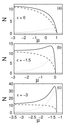
Figure 1: The total number of atoms (decreased by the factor $\Delta$) vs. the chemical potential in the units of $\hbar\omega_{\perp}/2$ (the solid line) corresponding to $a=0.01$ and $\kappa=1$. The dashed and dotted lines give the number of atoms in the $u$- and $v$-condensates, respectively. In panel (a) the unstable stationary state is attained in the limit of $\mu\to-\infty$, while in panels (b) and (c) the unstable states appear for finite negative $\mu$ where $\partial N/\partial\mu>0$. The stable states correspond to $\partial N/\partial\mu<0$.

Let us determine the energy of the stationary states. In the coupled-mode approximation the energy (measured in the units of $\Delta\hbar\omega_{\perp}/2$) reads

$$E=\int\mathrm{d}^{2}\vec{\rho}\,\left\{|\nabla u|^{2}+|\nabla v|^{2}+\rho^{2}(|u|^{2}+|v|^{2})+\varepsilon|v|^{2}-\kappa(uv^{*}+vu^{*})-\frac{|u|^{4}}{2}+a\frac{|v|^{4}}{2}\right\}.$$ (5)

Using the coupled-mode system (3) to express the kinetic energy of a stationary state one can reduce the expression for the total energy to the following

$$E=\mu N+\frac{1}{2}\int\mathrm{d}^{2}\vec{\rho}\,\left\{U^{4}-aV^{4}\right\}.$$ (6)

The numerically computed energy of the stationary state vs. the total number of atoms, corresponding to Fig. 1, is illustrated in Fig. 2 (to produce this figure we have computed the number of atoms and the energy separately by using the numerically found stationary states). It is seen that the collapsing states with $N$ approaching the limit value $N_{\mathrm{th}}$ have the energy approaching zero. Note the change of sign of the derivative ${\partial E}/{\partial N}$ at $N=0$ as we decrease the zero-point energy difference in panels (a) through (c). (The fact that the zero-point energy difference is negative in figures 2(b) and (c) is a mere coincidence, see also figure 4.)

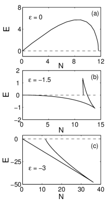
Figure 2: The energy of the stationary state (in the units of $\Delta\hbar\omega_{\perp}/2$) vs. the total number of atoms (decreased by the factor $\Delta$) corresponding to figure 1. The almost straight line in panel (c) contains the ground state of the system stable with respect to collapse.

The derivative ${\partial E}/{\partial N}$ at $N=0$ can be found analytically as follows. For $\epsilon=\mu_{\mathrm{bif}}-\mu\to 0$ the balance of the terms $U^{3}$ and $\mu U$ and the linear coupling of the $U$ and $V$ components in equation (3a) give $U,V\sim\sqrt{|\epsilon|}$, while the characteristic radius of the solution is fixed by the trap size. Hence, from equation (6) we conclude that $E=\mu_{\mathrm{bif}}N+\mathcal{O}(\epsilon^{2})$ due to the fact that $N\sim|\epsilon|$ in this limit. Thus ${\partial E}/{\partial N}=\mu_{\mathrm{bif}}+\mathcal{O}(\epsilon)$.

If the sign of ${\partial E}/{\partial N}$ at $N=0$ is negative, that is $\varepsilon\leq\varepsilon_{0}$ with $\varepsilon_{0}={\kappa^{2}}/{2}-2$, and the maximal value $N_{\mathrm{m}}$ of the number of atoms in a stationary state exceeds $N_{\mathrm{th}}$ then the ground state of the system with $N>N_{\mathrm{th}}$ is secured from collapse by an energy barrier. Indeed, first of all as either $\mu\to-\infty$ or $\mu\to\mu_{\mathrm{bif}}$ we have $E\to 0$. Hence, for $\mu_{\mathrm{bif}}<0$ the function $E=E(N)$ has a local minimum at $N_{\mathrm{m}}$, where it assumes a negative value. Consider the stable stationary solutions with negative energy and the number of atoms $N_{\mathrm{th}}<N<N_{\mathrm{m}}$ (such solutions lie on the almost straight line of the curve $E=E(N)$ in Fig. 2(c)). The system in such a state can collapse if some finite amount of energy is passed to the condensates by an external perturbation, i.e. there is an energy barrier for collapse.

In an attempt to understand the energy barrier for collapse let us first try to determine the effective interaction in the coupled-mode system. The effective interaction depends on the number of atoms and the double-well trap parameters. An example of the effective interaction switch from repulsive to attractive is given in Fig. 3, which is a part of Fig. 1(c) zoomed in about $\mu_{\mathrm{bif}}$. The interaction changes sign at ${\partial\mu}/{\partial N}=0$ when a zero eigenvalue appears the linear stability spectrum (see Eqs. (10)-(12) in the Appendix; the positivity of the linear stability spectrum is a sign of the effective repulsion in the system, see below). As shown in the Appendix, the stationary states are unconditionally stable when the effective interaction is repulsive.

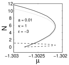
Figure 3: Zoomed in part of figure 1(c) about $\mu=\mu_{\mathrm{bif}}$ which manifests the effective repulsion in the coupled-mode system in the vicinity of the bifurcation point. Here the axis units are as in figure 1.

The effective interaction can be analytically studied as $\epsilon=\mu_{\mathrm{bif}}-\mu\to 0$. First we use equation (3b) to express $V$ in terms of $U$ and its derivatives as follows

$$V=\kappa\beta U-a\kappa^{3}\beta^{4}U^{3}+\kappa\beta^{2}(\nabla^{2}+2-\rho^{2})U+3a^{2}\kappa^{5}\beta^{7}U^{5}+\ldots,$$ (7)

where $\beta=(\varepsilon+2-\mu)^{-1}$ and the higher order terms are represented by dots. Equation (7) is derived in a similar way as an analogous equation for the one-dimensional coupled mode system in Ref. DW1D , one only has to replace the second-order differential operator by $\nabla^{2}+2-\rho^{2}$ and $\mu$ by $\mu-2$. Following Ref. DW1D we substitute the expression (7) into equation (3a) and get

$$-\epsilon\left(1+\frac{\kappa^{2}}{\mu_{0}^{2}}\right)U+\left(1+\frac{\kappa^{2}}{\mu_{0}^{2}}\right)(\nabla^{2}+2-\rho^{2})U+\left(1-\frac{a\kappa^{4}}{\mu_{0}^{4}}\right)U^{3}+\frac{3a^{2}\kappa^{6}}{\mu_{0}^{7}}U^{5}+\ldots=0,$$ (8)

where $\mu_{0}\equiv 2+\varepsilon/2+\sqrt{\varepsilon^{2}/4+\kappa^{2}}$.

In the limit of the small amplitude solution the interaction sign is defined by the coefficient at the cubic term (apart from the exceptional case of zero). The effective interaction is attractive for $\varepsilon>\varepsilon_{\mathrm{int}}$ with $\varepsilon_{\mathrm{int}}=\kappa(a^{1/4}-a^{-1/4})$. This formula accounts for Fig. 3, since there we have $\varepsilon<\varepsilon_{\mathrm{int}}=-2.85$.

Comparison of Figs. 2(c) and 3 leads to the conclusion that the energy barrier for collapse in the system cannot be explained by the repulsive effective interaction. Indeed, the interval of the $N$ axis occupied by the stable ground states in Fig. 2(c) is much wider that of the repulsive interaction in Fig. 3.

Moreover, we get $\varepsilon_{\mathrm{int}}\leq\varepsilon_{0}$ for $\kappa\geq\kappa_{\mathrm{cr}}$, where $\kappa_{\mathrm{cr}}\equiv\sqrt{Q^{2}+4}-Q$ with $Q=a^{-1/4}-a^{1/4}$. Hence, for $\kappa\geq\kappa_{\mathrm{cr}}$ and $\varepsilon_{\mathrm{int}}\leq\varepsilon\leq\varepsilon_{0}$ there are stable ground states with negative energy in the limit $\mu\to\mu_{\mathrm{bif}}$, while the effective interaction is attractive. An example is provided in Fig. 4, where $\varepsilon=1$ while $\varepsilon_{\mathrm{int}}=-10.65$ and $\varepsilon_{0}=5$.

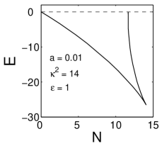
Figure 4: An example of the energy barrier for collapse in the system with the attractive effective interaction. In this case $\varepsilon_{\mathrm{int}}=-10.56$, while $\varepsilon_{0}=5$. Here the axis units are as in figure 2.

Fig. 4 also is a counterexample to the possible explanation of stability of the ground state with a negative energy by the fact that the repulsive condensate has a lower zero-point energy ($\varepsilon<0$), i.e. is placed in the lower well of the double-well trap.

To understand the existence and stability of the stationary states with negative energy let us examine the expression for the energy (6). As shown above, for small number of atoms, i.e. for $\mu\to\mu_{\mathrm{bif}}$, the linear part of the r.h.s. of equation (6) is dominant. But for a large number of atoms the nonlinear part must dominate. In this case, it is seen that the energy decreases with increase of the number of atoms if the term $aV^{4}$ is dominant in the integral (it is important to note that the two terms in the integral on the r.h.s. of formula (6) are due to an interplay of the atomic interactions, the kinetic energy, the quantum tunneling and the zero-point energy difference in the system, since we have expressed the kinetic energy of the condensates in terms of the other energies to obtain formula (6)). Indeed, comparing the figures 1 and 2 we see that when $\partial E/\partial N<0$ a much larger share of atoms is confined in the repulsive condensate (figures 1(c) and 2(c)). Therefore, such a stationary state does not collapse, since the energy would increase if some of the atoms tunnel from the repulsive condensate to the attractive one. This causes the energy barrier for collapse.

The stable ground states with negative energy in the system of tunnel-coupled repulsive and attractive two-dimensional condensates are analogous to the “unusual solitons” in the one-dimensional case DW1D which also appear close to the bifurcation point. The unusual soliton is a bright soliton which has a much larger share of atoms confined in the repulsive condensate.

III Conclusion

In conclusion, we have found the ground states in the system of tunnel-coupled repulsive and attractive condensates, which are stable with respect to collapse. The coupled-mode approximation have been used and is justified by the condensates being far separated in the wells of the double-well trap. We predict the existence of an energy barrier for collapse in the system, which is related to the appearance of the stable ground state with a negative energy. The condensates in such a ground state can collapse only if they are externally excited with a finite amount of energy being passed to the system.

The ground state with a negative energy is characterized by a large share of atoms trapped in the repulsive condensate. The contribution to the energy from the attractive condensate is positive, whereas from the repulsive one is negative (the contribution of each condensate is determined as the result of an interplay between the kinetic energy, the interaction energy and the zero-point energy, additionally there is the coupling energy due to the quantum tunneling). Therefore, the energy increases if some atoms tunnel from the repulsive to the attractive condensate. This explains the existence of the energy barrier for collapse in the system. The energy barrier appears for a wide region of the parameters space under the condition that the zero-point energy difference is less than a threshold value. The latter depends on the tunneling coefficient and can be both positive and negative (i.e. the condensate with repulsion can be placed in the upper well of the asymmetric double-well trap).

As is known, the Gross-Pitaevskii equation is sufficient to describe stable stationary states of the Bose-Einstein condensates at zero temperature, due to the similarity between the Bogoliubov-de Gennes equations and the equations describing evolution of a linear perturbation of the condensate order parameter APPL . Therefore, at zero temperature, given that the cloud of non-condensed atoms can be neglected, the energy barrier for collapse phenomenon can be observed.

IV Acknowledgements

This work was supported by the CNPq-FAPEAL grant of Brazil.

Appendix A Linear stability analysis

We will consider only the axially symmetric stationary points of system (3): $u=e^{-i\mu T}U(\rho)$ and $v=e^{-i\mu T}V(\rho)$. Stability can be established by considering the eigenvalue problem associated with the linearized system. Writing the perturbed solution as follows

$$u=e^{-i\mu T}\left\{U(\rho)+e^{-i\Omega T}\mathcal{U}(\vec{\rho})\right\},\quad v=e^{-i\mu T}\left\{V(\rho)+e^{-i\Omega T}\mathcal{V}(\vec{\rho})\right\},$$ (9)

where $(\mathcal{U}$,$\mathcal{V})$ is a small perturbation mode with frequency $\Omega$, one arrives at the following linear problem for the eigenfrequency:

$$-i\Omega\left(\begin{array}[]{c}\mathcal{U}_{R}\\ \mathcal{V}_{R}\end{array}\right)=\Lambda_{0}\left(\begin{array}[]{c}\mathcal{U}_{I}\\ \mathcal{V}_{I}\end{array}\right),\quad i\Omega\left(\begin{array}[]{c}\mathcal{U}_{I}\\ \mathcal{V}_{I}\end{array}\right)=\Lambda_{1}\left(\begin{array}[]{c}\mathcal{U}_{R}\\ \mathcal{V}_{R}\end{array}\right),$$ (10)

with

$$\Lambda_{0}=\left(\begin{array}[]{cc}L^{(u)}_{0}&-\kappa\\ -\kappa&L^{(v)}_{0}\end{array}\right),\quad\Lambda_{1}=\left(\begin{array}[]{cc}L^{(u)}_{1}&-\kappa\\ -\kappa&L^{(v)}_{1}\end{array}\right).$$ (11)

Here the scalar operators are defined as follows

$$L^{(u)}_{0}=-(\nabla^{2}+U^{2}+\mu)+\rho^{2},\quad L^{(u)}_{1}=-(\nabla^{2}+3U^{2}+\mu)+\rho^{2},\quad L^{(v)}_{0}=-(\nabla^{2}-aV^{2}+\mu-\varepsilon)+\rho^{2},$$

$$\quad L^{(v)}_{1}=-(\nabla^{2}-3aV^{2}+\mu-\varepsilon)+\rho^{2}.$$ (12)

First of all, the matrix operator $\Lambda_{0}$ is non-negative for positive stationary solutions, i.e. satisfying $UV>0$. Indeed, the scalar operators on the main diagonal of $\Lambda_{0}$ can be cast as follows

$$L^{(u)}_{0}=-\frac{1}{U}\nabla U^{2}\nabla\frac{1}{U}+\kappa\frac{V}{U},\quad L^{(v)}_{0}=-\frac{1}{V}\nabla V^{2}\nabla\frac{1}{V}+\kappa\frac{U}{V},$$

what can be easily verified by direct calculation. Therefore the scalar product of $\Lambda_{0}$ with any vector $X=(X_{1}(\vec{\rho}),X_{2}(\vec{\rho}))$ is non-negative:

$$\langle X|\Lambda_{0}|X\rangle=\int\mathrm{d}^{2}\vec{\rho}\,\left\{X_{1}^{*}L^{(u)}_{0}X_{1}+X_{2}^{*}L^{(v)}_{0}X_{2}-\kappa(X_{1}^{*}X_{2}+X_{2}^{*}X_{1})\right\}$$

$$\geq\kappa\int\mathrm{d}^{2}\vec{\rho}\,\left|X_{1}\sqrt{\frac{V}{U}}-X_{2}\sqrt{\frac{U}{V}}\,\right|^{2}\geq 0.$$

Here we have used the positivity of the operators $-\frac{1}{U}\nabla U^{2}\nabla\frac{1}{U}$ and $-\frac{1}{V}\nabla V^{2}\nabla\frac{1}{V}$. The operator $\Lambda_{0}$ has one zero mode given by the stationary point itself: $Z=(U,V)$, $\Lambda_{0}Z=0$. Non-negativity of $\Lambda_{0}$ is an essential fact for the following. Thus the non-positive solutions, i.e. satisfying the inequality $UV<0$, are discarded from the consideration.

The lowest eigenfrequency of the linear stability problem can be found also by minimizing the following quotient

$$\Omega^{2}=\mathrm{min}\frac{\langle X|\Lambda_{1}|X\rangle}{\langle X|\Lambda^{-1}_{0}|X\rangle}$$ (13)

in the space orthogonal to the zero mode of $\Lambda_{0}$: $\langle Z|X\rangle=0$ (here $\langle X|Y\rangle\equiv\int\mathrm{d}^{2}\vec{\rho}\,(X^{*}_{1}Y_{1}+Y_{2}X^{*}_{2})$). Equation (13) follows from the eigenvalue problem rewritten as $\Lambda_{0}\Lambda_{1}X=\Omega^{2}X$ with $X=(\mathcal{U}_{R},\mathcal{V}_{R})$.

The imaginary eigenfrequencies $\Omega$, which mean instability, appear due to negative eigenvalues of the operator $\Lambda_{1}$. If there is just one negative eigenvalue, then the Vakhitov-Kolokolov (VK) stability criterion ${\partial N}/{\partial\mu}<0$ applies, which can be established by a simple repetition of the arguments presented, for instance, in Ref. PhysD . The limit on the number of negative eigenvalues is related to the fact that the minimization of the quotient in equation (13) is subject to only one orthogonality condition, thus only one negative direction can be eliminated by satisfying this orthogonality condition.

To apply the VK criterion for stability of the stationary points in the 2D case (as compared to the 1D case PhysD ) one has to rely on numerics to establish the number of negative eigenvalues of the operator $\Lambda_{1}$. The following simple strategy was used. The eigenvalue problem was reformulated in the polar coordinates $(\rho,\theta)$ and the operators were expanded in Fourier series with respect to $\theta$ by the substitution: $\nabla^{2}\to\nabla^{2}_{\rho}-n^{2}/\rho^{2}$, where $\nabla^{2}_{\rho}=\partial^{2}_{\rho}+\rho^{-1}\partial_{\rho}$. Noticing that the orbital operators $\Lambda_{1,n}=\Lambda_{1}(\nabla^{2}\to\nabla^{2}_{\rho}-n^{2}/\rho^{2})$ are ordered as follows $\Lambda_{1,n+1}\geq\Lambda_{1,n}$, we have checked for the negative eigenvalues of the first two orbital operators with $n=0,1$. It turns out that $\Lambda_{1,1}$ is always positive, while the operator $\Lambda_{1,0}$ has one negative eigenvalue or none (the latter corresponds to the effective repulsive interaction in the system). Thus the VK criterion applies in the former case, while in the latter one the stationary point is unconditionally stable.

References

- (1) L. P. Pitaevskii, Zh. Eksp. Teor. Fiz. 40, 646 (1961) [Sov. Phys. JETP 13, 451 (1961); E. P. Gross, Nuovo Cimento 20, 454 (1961); J. Math. Phys. 4, 195 (1963).
- (2) M. R. Andrews, C. G. Townsend, H.-J. Miesner, D.S. Durfee, D. M. Kurn, and W. Ketterle, Science 275, 637 (1997).
- (3) D. S. Hall, M. R. Matthews, C. E. Wieman, and E. A. Cornell, Phys. Rev. Lett. 81, 1543 (1998).
- (4) A. Röhrl, M. Naraschewski, A. Schenzle, and H. Wallis, Phys. Rev. Lett. 78, 4143 (1997).
- (5) A. J. Leggett, Rev. Mod. Phys. 73, 307 (2001).
- (6) W. Zhang, B. C. Sanders and A. Mann, J. Phys. I 6, 1411 (1996).
- (7) C. C. Bradley, C. A. Sackett, and R. G. Hulet, Phys. Rev. Lett 78, 985 (1997).
- (8) J. K. Chin, J. M. Vogels, and W. Ketterle, Phys. Rev. Lett. 90, 160405 (2003).
- (9) Yu. Kagan, A. E. Muryshev, and G. V. Shlyapnikov, Phys. Rev. Lett. 81, 933 (1998); M. Ueda and A. J. Leggett, Phys. Rev. Lett. 80, 1576 (1998).
- (10) A. Gammal, T. Frederico, and L. Tomio, Phys. Rev. A 64, 055602 (2001); A. Gammal, L. Tomio, and T. Frederico, Phys. Rev. A 66, 043619 (2002).
- (11) C. M. Savage, N. P. Robins, and J. J. Hope, Phys. Rev. A 67, 014304 (2003).
- (12) N. P. Robins, W. Zhang, E. A. Ostrovskaya, and Yu. S. Kivshar, Phys. Rev. A 64, 021601(R) (2001).
- (13) S. K. Adhikari, Phys. Rev. A 63, 043611 (2001); J. Phys. B: At. Mol. Opt. Phys. 34, 4231 (2001).
- (14) R. Roth and H. Feldmeier, Phys. Rev. A 65, 021603(R) (2002).
- (15) R. Roth, Physical Review A 66, 013614 (2002).
- (16) A. J. Moerdijk, B. J. Verhaar, and A. Axelsson, Phys. Rev. A 51, 4852 (1995).
- (17) M. Wouters, J. Tempere, and J. T. Devreese, Phys. Rev. A 68, 053603 (2003).
- (18) V. S. Shchesnovich, S. B. Cavalcanti, Stationary states in a pair of tunnel-coupled two-dimensional condensates with the scattering lengths of opposite sign, to appear in Progress in Soliton Research, Nova Science Publishers, Inc.
- (19) V. S. Shchesnovich, S. B. Cavalcanti, and R. A. Kraenkel Physical Review A 69, 033609 (2004).
- (20) V. S. Shchesnovich, B. A. Malomed and R. A. Kraenkel, Physica D 188, 213 (2004).
- (21) G. Fibich and G. Papanicolaou, SIAM J. Appl. Math. 60, 183 (1999).
- (22) Y. Castin and R. Dum, Phys. Rev. A 57, 3008 (1998).