Finite-size behaviour of the microcanonical specific heat

Abstract

For models which exhibit a continuous phase transition in the thermodynamic limit a numerical study of small systems reveals a non-monotonic behaviour of the microcanonical specific heat as a function of the system size. This is in contrast to a treatment in the canonical ensemble where the maximum of the specific heat increases monotonically with the size of the system. A phenomenological theory is developed which permits to describe this peculiar behaviour of the microcanonical specific heat and allows in principle the determination of microcanonical critical exponents.

1 Introduction

In recent years numerous studies investigated the possible differences between the microcanonical and the canonical treatment of a given system. It is now well accepted that in various cases the microcanonical and the canonical ensemble are not equivalent [1, 2, 3, 4, 5, 6, 7, 8]. For short-range interactions, the equivalence of the two ensembles holds in the infinite volume limit, but this is not the case in finite systems. For long-range interactions, as encountered for example in gravitational systems, the two ensembles remain inequivalent even for infinite systems.

Clearly, this inequivalence in finite systems makes the microcanonical analysis of possible signatures of phase transitions an important issue [2, 9, 10, 5, 11, 12]. For discontinuous phase transitions, the microcanonical analysis reveals typical small system signatures, as e. g. a back-bending of the caloric curve or the appearance of a negative specific heat. Negative heat capacities have indeed been measured in recent experiments on nuclear fragmentation [13] and on the melting of atomic clusters [14]. Similarly, intriguing features are also revealed in the microcanonical analysis of small systems which exhibit a continuous phase transition in the thermodynamic limit. Indeed, typical features of symmetry breaking, as e. g. the abrupt onset of a non-zero order parameter when the (pseudo-)critical point is approached from above or a diverging susceptibility, turn up already for finite systems [9]. This is in contrast to the canonical ensemble where singularities appear exclusively in the thermodynamic limit.

The fundamental quantity in a microcanonical analysis is the density of states or, equivalently, the microcanonical entropy. All relevant quantities can indeed be expressed by partial derivatives of the microcanonical entropy. For example, the susceptibility is proportional to the inverse of the curvature of the entropy surface. It is the existence of a point with vanishing curvature that is responsible for the divergent susceptibility observed in finite systems which have a continuous phase transition in the infinite volume limit.

In the present work we examine more closely the finite-size behaviour of the microcanonical specific heat in different classical spin systems. For systems with a continuous phase transition one expects that the maximum of the specific heat increases with increasing system size. This is indeed observed in the microcanonical analysis for not too small systems. For small system sizes, however, we observe a non-monotonic behaviour as the maximum of the specific head first decreases for increasing system sizes. This is again a property of the entropy surface as the microcanonical specific heat can be exclusively expressed by energy derivatives of the microcanonical entropy. In order to account for this peculiar behaviour we develop a phenomenological theory based on the analyticity of the entropy surface of finite systems.

The paper is organized as follows. In Section 2 we first discuss the definition of the temperature in the microcanonical ensemble. In the microcanonical ensemble various definitions of the temperature are possible, the different expressions becoming equivalent in the thermodynamic limit. The microcanonical specific heat, based on the expressions for the temperature, is the subject of Section 3. Numerical results obtained for two- and three-dimensional Ising models as well as for the two-dimensional three-state Potts model reveal a non-monotonic behaviour of the specific heat for increasing system sizes. The finite-size behaviour of the specific heat of microcanoncial systems is considered from a phenomenological point of view in Section 4 where a finite-size scaling theory is developed which explains the peculiar behaviour of the microcanonical specific heat of small systems. Finally, Section 5 gives our conclusions.

2 Temperature in the microcanonical ensemble

The density of states is the starting point for the statistical description of thermostatic properties in the different ensembles. For a magnetic system that is isolated from any environment the proper natural variables are the energy $E$ and the magnetisation $M$. The corresponding characteristic function of the isolated system is the microcanonical entropy

$$S(E,M,L^{-1})=\ln\Omega(E,M,L^{-1})$$ (1)

where $\Omega$ denotes the degeneracy of the macrostate $(E,M)$ and $L$ is the linear extention of the system. Here and in the following units with $k_{B}=1$ are used. The microcanonical analysis of finite classical spin systems starts from the microcanonical entropy density

$$s(e,m,L^{-1}):=\frac{1}{L^{d}}S(L^{d}e,L^{d}m,L^{-1})$$ (2)

of a system in $d$ dimensions with $N=L^{d}$ spins, where $e=E/N$ denotes the energy density and $m=M/N$ the magnetisation density. In the following the dependence on the system size is suppressed in order to improve readability.

Before investigating the microcanonical specific heat, we first have to discuss the definition of the temperature for finite systems in the microcanonical ensemble. In the thermodynamic limit canonically defined physical quantities and the corresponding microcanonical quantities have to become identical for systems with suitably short range forces. However, this requirement does not yield an unambiguous definition of the microcanonical temperature, leading to different physically plausible definitions in finite systems which all become equivalent in the thermodynamic limit.

The starting point is the canonical partition function

$$Z(\tilde{\beta},\tilde{h})=L^{2d}\int\mbox{d}e\,\int\mbox{d}m\,\exp\left\{L^{d}(s(e,m)-\tilde{\beta}e+\tilde{\beta}\tilde{h}m)\right\}$$ (3)

which is the Laplace transform of the density of states. Here the inverse canonical temperature $\tilde{\beta}$ and the applied magnetic field $\tilde{h}$ are external parameters which are imposed on the system by its environment. The canonical temperature and external field are denoted by a tilde in order to avoid any confusion with the microcanonical temperature and field defined in the following. The integral (3) can be evaluated in the limit $L\to\infty$ by means of the Laplace method. For a given inverse temperature $\tilde{\beta}$ and external magnetic field $\tilde{h}$ the dominant contributions to the integral arise from the maximum of the argument $g(e,m)=s(e,m)-\tilde{\beta}e+\tilde{\beta}\tilde{h}m.$ The equations $\partial_{e}g=0$ and $\partial_{m}g=0$ suggest the following definitions of the inverse microcanonical temperature:

$$\beta(e,m)=\partial_{e}s(e,m)$$ (4)

and of the microcanonical magnetic field:

$$\beta(e,m)h(e,m)=-\partial_{m}s(e,m).$$ (5)

Here and in the following the notation $\partial_{x}$ is used for the partial derivative $\partial/\partial x$. The inverse microcanonical temperature $\beta$ and magnetic field $h$ are conjugate variables of the natural variables $e$ and $m$ of the microcanonical approach and consequently depend on these. The definition (4) of the microcanonical temperature surface leads to the follwing definition of the temperature in equilibrium. Consider the spontaneous magnetisation $m_{\scriptsize\mbox{sp}}(e)$ of the magnetic system for a given energy $e$ that is defined by the condition $h(e,m)=0$ [9]. The temperature of the magnetic system in equilibrium is then obtained by evaluating the inverse temperature surface $\beta(e,m)$ at the equilibrium macrostate $(e,m_{\scriptsize\mbox{sp}}(e))$:

$$\beta_{\scriptsize\mbox{E}}(e):=\beta(e,m_{\scriptsize\mbox{sp}}(e))=\partial_{e}s(e,m)|_{m=m_{\scriptsize\mbox{sp}}(e)}.$$ (6)

This definition of the inverse temperature ensures ensemble equivalence between the canonical and microcanonical description, as can be seen using the Laplace method in the asymptotic limit $L\to\infty$. For finite $L$, however, the exponential in (3) cannot be approximated by the quadratic term of the Taylor expansion only. Higher order terms are necessary which render the integrand asymmetric. Consequently, the canonical mean values are shifted from the associated maximum of the entropy surface leading to the inequivalence of the canonical and the microcanoncial ensemble for finite system sizes.

We pause here for a moment to recall that the spontaneous magnetisation $m_{\scriptsize\mbox{sp}}(e)$ of a finite microcanonical magnetic system exhibits features which are typical of phase transitions. The spontaneous magnetisation of the Ising model in dimensions $d\geq 2$, for example, is zero above a well-defined transition energy $e_{\scriptsize\mbox{pc}}$ and becomes non-zero below $e_{\scriptsize\mbox{pc}}$. Close to this pseudo-critical energy the variation of the spontaneous magnetisation as a function of the deviation of $e$ from $e_{\scriptsize\mbox{pc}}$ is described by a square root function [9, 11]. This classical behaviour has its origin in the analyticity of the entropy surface for all finite systems [15, 16]. The appearance of a non-zero spontaneous magnetisation reflects the spontaneous breakdown of the global symmetry of the system and may be regarded as a precursor of the critical point of the infinite system [9, 11, 17]. Note that the specific entropy $s_{\infty}(e,m)$ in the thermodynamic limit is a concave function of its variables. In finite systems, however, this is not compulsory so that two maxima of the entropy can appear at non-zero magnetisations for a given energy.

Coming back to the canonical ensemble we remark that in absence of a magnetic field the partition function (3) simplifies to

$$Z(\tilde{\beta},\tilde{h}=0)=L^{d}\int\mbox{d}e\,\left(L^{d}\int\mbox{d}m\,\exp\left\{L^{d}s(e,m)\right\}\right)\exp\{-L^{d}\tilde{\beta}e\},$$ (7)

which leads to the definition

$$\exp\{L^{d}s_{\scriptsize\mbox{R}}(e)\}=L^{d}\int\mbox{d}m\,\exp\left\{L^{d}s(e,m)\right\}$$ (8)

of the reduced (specific) entropy $s_{\scriptsize\mbox{R}}(e)$. In the limit of large system sizes the dominant contributions to the integral (7) arise from the energy defined by the maximum of the argument $s_{\scriptsize\mbox{R}}(e)-\tilde{\beta}e$ for a given inverse canonical temperature $\tilde{\beta}$. This suggests the following alternative definition of an inverse (reduced) microcanonical temperature, namely

$$\beta_{\scriptsize\mbox{R}}(e)=\frac{\mbox{d}}{\mbox{d}e}s_{\scriptsize\mbox{R}}(e).$$ (9)

The thermal properties of the system are now obtained from the entropy function $s_{\scriptsize\mbox{R}}(e)$ rather than from the full entropy surface $s(e,m)$ depending on both the energy and the magnetisation.

To conclude this section the interrelation between the inverse temperatures $\beta_{\scriptsize\mbox{E}}(e)$ and $\beta_{\scriptsize\mbox{R}}(e)$ is briefly considered. In the asymptotic limit $L\to\infty$ the integral (8) is dominated by the entropy $s(e,m_{\scriptsize\mbox{sp}}(e))$, evaluated at the spontaneous magnetization $m_{\scriptsize\mbox{sp}}(e)$, as can again be seen by using the Laplace method. Therefore, the entropy $s_{\scriptsize\mbox{R}}(e)$ is given by $s(e,m_{\scriptsize\mbox{sp}}(e))$ for asymptotically large system sizes $L$ and one gets

$$\beta_{\scriptsize\mbox{R}}(e)\stackrel{{\scriptstyle L\to\infty}}{{\sim}}\frac{\mbox{d}}{\mbox{d}e}s(e,m_{\scriptsize\mbox{sp}}(e)).$$ (10)

Carrying out this differentiation we obtain the relation

$$\beta_{\scriptsize\mbox{R}}(e)\stackrel{{\scriptstyle L\to\infty}}{{\sim}}\frac{{\partial}}{{\partial}e}s(e,m)|_{m=m_{\scriptsize\mbox{sp}}(e)}+\frac{{\partial}}{{\partial}m}s(e,m)|_{m=m_{\scriptsize\mbox{sp}}(e)}\frac{\mbox{d}}{\mbox{d}e}m_{\scriptsize\mbox{sp}}(e).$$ (11)

As $\partial_{m}s(e,m)$ is zero at $(e,m_{\scriptsize\mbox{sp}}(e))$ the second term vanishes and one is left with $\beta_{\scriptsize\mbox{R}}(e)\sim\beta_{\scriptsize\mbox{E}}(e)$. The full entropy surface $s(e,m)$ and the reduced entropy function $s_{\scriptsize\mbox{R}}(e)$ will therefore lead to the same equilibrium temperature in the asymptotic limit $L\to\infty$. For finite $L$, however, $\beta_{\scriptsize\mbox{E}}(e)$ is significantly different from $\beta_{\scriptsize\mbox{R}}(e)$.

3 Microcanonical specific heat

3.1 General discussion

Once the inverse temperature $\beta$ of a microcanonical system is evaluated — here $\beta$ may be $\beta_{\scriptsize\mbox{E}}$ or $\beta_{\scriptsize\mbox{R}}$ — one can calculate the specific heat which is generally defined by $c=\mbox{d}u/\mbox{d}T$ with $u$ and $T=1/\beta$ being the energy and the temperature of the system. For the microcanonical specific heat as a function of the energy of the system this gives

$$c(e)=-(\beta(e))^{2}\left(\frac{\mbox{d}\beta(e)}{\mbox{d}e}\right)^{-1}=-\left(\frac{\mbox{d}s}{\mbox{d}e}\right)^{2}\left(\frac{\mbox{d}^{2}s}{\mbox{d}e^{2}}\right)^{-1}.$$ (12)

The discussed ambiguity in the definition of the microcanonical temperature leads also to different expressions for the specific heat in finite systems. However, they converge towards the same limit function in the thermodynamic limit.

In the following we discuss the finite-size behaviour of the specific heat arising from the temperature $\beta_{\scriptsize\mbox{R}}(e)$ in different classical spin models (from now on we drop the subscript R in order to avoid unnecessary notation). Note that this is the definition of the specific heat that is the most relevant for experiments where usually the energy is considered as the unique natural variable corresponding to systems to which no external field is applied. Specifically, we study three models undergoing a continuous phase transition in the thermodynamic limt: the two- and and the three-dimensional Ising model as well as the three-state Potts model in two dimensions. The nearest neighbour Ising model is defined by the Hamiltonian

$$\mathcal{H}=-\sum_{\left<i,j\right>}\sigma_{i}\sigma_{j},$$ (13)

where the summation over nearest neighbour pairs is indicated by $\left<i,j\right>$ and the spin $\sigma_{i}$ at site $i$ can be in the states $\sigma_{i}=\pm 1$. In the present study Ising models defined on the square and on the cubic lattices are considered. The three-state Potts model is a generalisation of the Ising model where the Potts spins $\sigma_{i}$ take on the values $1,2,3$. The Hamiltonian is given by

$$\mathcal{H}=-\sum_{\left<i,j\right>}\delta_{\sigma_{i},\sigma_{j}},$$ (14)

where $\delta_{\sigma_{i},\sigma_{j}}=1$ when the spins located at the neighbouring sites $i$ and $j$ have the same value and zero otherwise. For the Potts model we only consider the square lattice.

In finite systems the appearance of a continuous phase transition in the thermodynamic limit is signaled by a maximum in the specific heat which becomes more and more pronounced when the system size is increased. This behaviour of the specific heat is due to a maximum of the second derivative of $s(e)$ which is negative everywhere and tends to zero for increasing system sizes from below. The position of the maximum of the second derivative of $s(e)$ defines a pseudo-critical energy $e_{\scriptsize\mbox{pc}}$ of the finite system. At the same time the microcanonical inverse temperature $\beta_{\scriptsize\mbox{pc}}:=\beta(e_{\scriptsize\mbox{pc}})$ evaluated at the energy $e_{\scriptsize\mbox{pc}}$ converges towards the critical value $1/T_{\scriptsize\mbox{c}}$ when $L$ tends to infinity.

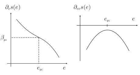
Figure 1: Schematic depiction of the first two derivatives of the reduced entropy near the pseudo-critical energy of a finite system. The pseudo-critical energy $e_{\scriptsize\mbox{pc}}$ corresponds to an inverse temperature $\beta_{\scriptsize\mbox{pc}}$ (left). The derivative $\partial_{ee}s$ has a maximum at $e_{\scriptsize\mbox{pc}}$ (right).

The behaviour just described, which is schematically sketched in figure 1, is indeed observed in the different models for not too small system sizes. For very small systems, however, our numerical results reveal an unexpected non-monotonic behaviour of the specific heat, as discussed in the next subsection.

3.2 Numerical results

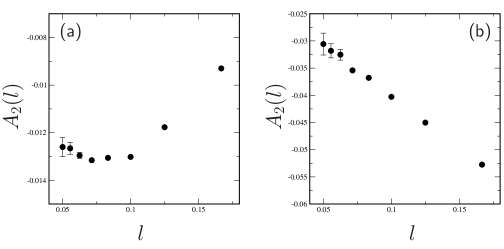
Figure 2: Evolution of the coefficient $A_{2}(l)$ for finite three-dimensional Ising systems with periodic boundary conditions (a) and open boundaries (b). The modulus of the coefficient $A_{2}(l)$ of the system with periodic boundary conditions has a plateau and becomes smaller again for small systems. In the thermodynamic limit $l\to 0$ both curves have to extrapolate to $A_{2}=0$.

In this subsection the specific heat of finite Ising and Potts systems is investigated numerically for both periodic and open boundary conditions. To obtain the numerical data we used a recently proposed very efficient method for the direct computation of the density of states [11]. Specifically, we discuss in the following the value $\partial_{ee}s(e_{\scriptsize\mbox{pc}},L^{-1})$ of the second derivative of the entropy evaluated at the pseudo-critical energy $e_{\scriptsize\mbox{pc}}$. For later convenience this value is denoted by $A_{2}(l)$ where $l:=L^{-1}$ is the inverse system size:

$$A_{2}(l)=\partial_{ee}s(e_{\scriptsize\mbox{pc}},l).$$ (15)

The coefficient $A_{2}(l)$ of finite three-dimensional Ising systems is shown in figure 2. With periodic boundary conditions the coefficient $A_{2}(l)$ shows a back-bending as its modulus first increases for increasing $l$ (i. e. decreasing system sizes) and then decreases for very small systems, see figure 2a. This intriguing and unexpected back-bending is not observed in the system with open boundaries.

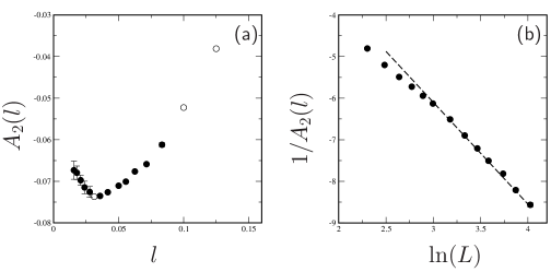
Figure 3: Evolution of the coefficient $A_{2}(l)$ for finite Ising models in two dimensions with periodic boundary conditions (a) and free boundaries (b). The open circles in (a) display exactly evaluated data. The coefficient $A_{2}(l)$ bends back for small systems only for periodic boundary conditions. For the system with open boundaries a logarithmic plot shows that the coefficient $A_{2}(l)$ evolves logarithmically for large systems (see also section 4).

Similarly, the coefficient $A_{2}(l)$ of the two-dimensional Ising model with periodic boundary conditions also exhibits this back-bending for very small system sizes, whereas again no back-bending is observed for open boundaries, see figure 3. In case of the systems with linear extensions $L=8,10$ and $32$ and periodic boundaries the numericaly determined data can be compared to exactly computed data [18, 19, 20]. This is also indicated in figure 3.

Naturally, the back-bending of the coefficient $A_{2}(l)$ directly affects the behaviour of the microcanonical specific heat of small systems as can be seen from equations (15) and (12). Indeed, the maximum of the specific heat first decreases with growing system size before increasing again, thus yielding a divergence in the thermodynamic limit. This decrease of the specific heat of small microcanonical systems is displayed in figure 4 for the three-dimensional Ising model with periodic boundary conditions. It is worth noting that such a peculiar behaviour of the specific heat of small systems is not observed in the canonical ensemble (see, e. g. [18, 21, 22]).

Figure 4: Evolution of the microcanonical specific heat for small three-dimensional Ising systems with periodic boundary conditions. The maximum decreases for increasing system size.

Finally, figure 5 displays the evolution of the coefficient $A_{2}(l)$ for finite two-dimensional three-state Potts models for both periodic and open boundary conditions. The back-bending is strongly pronounced for periodic boundaries and is in this case also visible, but less developed, for free boundaries. For large systems the coefficient $A_{2}(l)$ eventually approaches zero reflecting the appearance of a continuous transition in the infinite system.

Figure 5: Evolution of the coefficient $A_{2}(l)$ for finite three-state Potts models in two dimensions with periodic boundary conditions (a) and free boundaries (b). For both boundary conditions the coefficient $A_{2}(l)$ bends back for small systems.

4 Phenomenological theory for finite systems

In this section the behaviour of the specific heat of finite microcanonical systems is investigated from a phenomenological point of view. As discussed in the following this leads to a theoretical description that accounts for the peculiar behaviour of the microcanonical specific heat described in the previous section.

The specific heat of the infinite Ising or Potts systems diverges at the critical point $e_{\scriptsize\mbox{c},\infty}$. For a system with a power law singularity the specific heat has the form

$$c_{\infty}(e)\sim|e-e_{\scriptsize\mbox{c},\infty}|^{-\alpha_{\varepsilon}}$$ (16)

in the vicinity of the critical point, where $\alpha_{\varepsilon}$ denotes the microcanonical critical exponent. The specific entropy of the infinite system contains a singular part that is a generalised homogeneous function in the vicinity of $e_{\scriptsize\mbox{c},\infty}$ characterised by the degree of homogeneity $a_{\varepsilon}$ [9]. The microcanonical critical exponent $\alpha_{\varepsilon}$ is related to $a_{\varepsilon}$ by

$$\alpha_{\varepsilon}=\frac{1-2a_{\varepsilon}}{a_{\varepsilon}}=\frac{\alpha}{1-\alpha}$$ (17)

with $\alpha$ being the critical exponent of the canonical specific heat [9]. Similarly, the microcanonical critical exponent $\nu_{\varepsilon}$ of the correlation length can be expressed as

$$\nu_{\varepsilon}=\frac{1}{da_{\varepsilon}}=\frac{\nu}{1-\alpha}$$ (18)

where the dimensionality of the system is again denoted by $d$.

The discussion of finite-size scaling relations of the specific heat starts from the decomposition

$$s(\varepsilon,l)=s_{\scriptsize\mbox{r}}(\varepsilon,l)+s_{\scriptsize\mbox{s}}(\varepsilon,l)\;$$ (19)

of the entropy of a finite system into a regular and a singular part. The deviation of the energy from the pseudo-critical energy is denoted by $\varepsilon:=e-e_{\scriptsize\mbox{pc}}$, where $l$ again is the inverse system size. The singular and regular parts of the entropy of the finite systems are chosen to approach the corresponding singular and regular part of the entropy of the infinite lattice:

$$\lim_{l\to 0}s_{\scriptsize\mbox{s/r}}(\varepsilon,l)=s_{\infty,\scriptsize\mbox{s/r}}(\varepsilon).$$ (20)

Note that the singular part of the entropy of a finite system is an analytic function due to the analyticity of thermodynamic potentials of finite systems. The singular part $s_{\scriptsize\mbox{s}}(\varepsilon,l)$ is assumed to obey the scaling assumption

$$s_{\scriptsize\mbox{s}}(\varepsilon,l)=\frac{1}{\lambda}s_{\scriptsize\mbox{s}}(\lambda^{a_{\varepsilon}}\varepsilon,\lambda^{1/d}l)$$ (21)

with a positive re-scaling factor $\lambda$ and the degree of homogeneity $a_{\varepsilon}$ discussed above. The ansatz (21) for the finite-size behaviour of the singular part of the microcanonical entropy of finite systems does not account for additional finite-size corrections that arise from the contributions of irrelevant scaling fields. The qualitative picture that is developed in the following can be extended to include those contributions as well. Differentiating the finite-size scaling assumption (21) with respect to the re-scaling factor $\lambda$ and setting $\lambda=1$ afterwards gives rise to the differential equation

$$s_{\scriptsize\mbox{s}}(\varepsilon,l)=a_{\varepsilon}\varepsilon\partial_{\varepsilon}s_{\scriptsize\mbox{s}}(\varepsilon,l)+\frac{1}{d}\,l\partial_{l}s_{\scriptsize\mbox{s}}(\varepsilon,l)$$ (22)

for the singular part of the reduced entropy.

The entropy of a finite system is analytic [16] and therefore $s_{\scriptsize\mbox{s}}$ can be expanded with respect to the energy deviation $\varepsilon$, yielding the series expansion

$$s_{\scriptsize\mbox{s}}(\varepsilon,l)=B_{0}(l)+\sum_{n=1}^{\infty}\frac{1}{n}B_{n}(l)\varepsilon^{n}.$$ (23)

From equation (22) the differential equation

$$B_{n}(l)=na_{\varepsilon}B_{n}(l)+\frac{1}{d}\,l\partial_{l}B_{n}(l)$$ (24)

is obtained for the expansion coefficients $B_{n}(l)$, $n=0,1,\ldots$ This differential equation has the solution

$$B_{n}(l)=B_{n}^{(0)}l^{d(1-na_{\varepsilon})}$$ (25)

where the $B_{n}^{(0)}$ are size-independent coefficients. Similarly, the regular part of the reduced entropy can be expanded into the series

$$s_{\scriptsize\mbox{r}}(\varepsilon,l)=C_{0}(l)+\sum_{n=1}^{\infty}\frac{1}{n}C_{n}(l)\varepsilon^{n}.$$ (26)

As the regular part of the entropy of the infinite system is also analytic, it is natural to assume that the coefficients are regular functions in $l$ so that the $C_{n}(0)$ are the expansion coefficients of the regular part of the entropy of the infinite system. Mathematically speaking, the limiting procedure $l\to 0$ and the summation in (26) can be interchanged. This assumption is not possible for the singular part whose limit in the infinite system is non-analytic.

Taking everything together we obtain that the expansion of the total entropy of a finite system is of the form

$$s(\varepsilon,l)=s_{0}(l)+\sum_{n=1}^{\infty}\frac{1}{n}\left(B_{n}^{(0)}l^{d(1-na_{\varepsilon})}+C_{n}(l)\right)\varepsilon^{n}.$$ (27)

To proceed further let us consider the vicinity of the pseudo-critical point $e_{\scriptsize\mbox{pc}}$ of the finite system of inverse length $l$. From a Taylor expansion we obtain (with $\varepsilon=e-e_{\scriptsize\mbox{pc}}$)

$$s(\varepsilon,l)=s_{0}(l)+\beta_{\scriptsize\mbox{pc}}\varepsilon+\frac{1}{2}A_{2}(l)\varepsilon^{2}+\frac{1}{4}A_{4}(l)\varepsilon^{4}+\ldots$$ (28)

where the coefficients of the second and fourth order terms,

$$A_{2}(l)=B_{2}^{(0)}l^{\frac{\alpha_{\varepsilon}}{\nu_{\varepsilon}}}+C_{2}(l)$$ (29)

and

$$A_{4}(l)=B_{4}^{(0)}l^{\frac{\alpha_{\varepsilon}-2}{\nu_{\varepsilon}}}+C_{4}(l),$$ (30)

involve the critical exponents of the microcanonical system.

The coefficient $A_{2}(l)$ of the second degree term is of particular interest as it describes the evolution of the microcanonical specific heat at the pseudo-critical energy $e_{\scriptsize\mbox{pc}}$. Indeed, the curvature at $e_{\scriptsize\mbox{pc}}$ as a function of the system size is given by

$$\partial_{\varepsilon\varepsilon}s(\varepsilon=0,l)=A_{2}(l)=B_{2}^{(0)}l^{\frac{\alpha_{\varepsilon}}{\nu_{\varepsilon}}}+C_{2}(l)<0.$$ (31)

As the function $C_{2}(l)$ is regular and has to vanish in the thermodynamic limit ($l\to 0$) in order to produce a diverging specific heat at the critical point $e_{{\scriptsize\mbox{c}},\infty}$ of the infinite system, it has to be of the form

$$C_{2}(l)=v_{1}l+\frac{1}{2}v_{2}l^{2}+\ldots$$ (32)

for small $l$. For a continuous phase transition the coefficient $A_{2}(l)$ is negative for all inverse system sizes $l$ (see equations (31) and (12)), therefore, the coefficient $B_{2}^{(0)}$ is also negative as it is the dominating one for the asymptotic limit of vanishing $l$. However, the sign of the coefficient $C_{2}(l)$ is not further restricted. The possible evolutions of the coefficient $A_{2}(l)$ depending on the sign and variation of $C_{2}(l)$ are schematically shown in figure 6. A back-bending of the function $A_{2}(l)$ for decreasing system sizes can be caused by a large enough positive coefficient $C_{2}(l)$. The resulting minimum in $A_{2}$(l) has the consequence that the maximum of the specific heat of small systems decreases with increasing systems size $L$ and increases again in the limit of large systems. This is exactly what we observe numerically. Thus, the phenomenological viewpoint developed in this section accounts for the peculiar behaviour of the specific heat of small microcanonical systems reported in section 3.2.

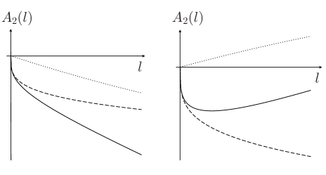
Figure 6: Schematic discussion of the possible size-dependence of the expansion coefficient $A_{2}(l)$ (solid lines) of the reduced entropy function. Shown are two cases, namely a negative (left) and positive (right) contribution $C_{2}(l)$. For small $l$ the variation is determined by the sum of the singular contribution $B_{2}(l)$ governed by the ratio $\alpha_{\varepsilon}/\nu_{\varepsilon}$ (dashed lines) and the contributions from $C_{2}(l)$ (dotted lines). For a rapidly growing positive contribution $C_{2}(l)$ the coefficient can have a minimum (right).

Finally, let us note that the consideration of the limit $l\to 0$ (i. e. $L\to\infty$) allows in principle the determination of the ratio $\alpha_{\varepsilon}/\nu_{\varepsilon}$ (see [23] for another recent discussion of this point). In the limit of large systems the evolution of the coefficient $A_{2}(l)$ as a function of the inverse system size $l$ is governed by the ratio $\alpha_{\varepsilon}/\nu_{\varepsilon}$. In figure 7 a double-logarithmic plot of the coefficient $|A_{2}(l)|$ is shown for the Potts system with periodic boundary conditions. The data for large systems is in good approximation described by a straight line. The slope of this line is an estimate of the exponent ratio $\alpha_{\varepsilon}/\nu_{\varepsilon}$. From our data we obtain the slope $0.42\pm 0.03$ which has to be compared with the exactly known value $2/5$. The evolution of the coefficient $A_{2}(l)$ for large system sizes is indeed determined by the critical exponent ratio $\alpha_{\varepsilon}/\nu_{\varepsilon}$. Hence, the microcanonical analysis of the evolution of physical quantities of finite systems allows, in principle, the determination of the true critical exponents characterising the critical behaviour of the infinite system (see [11, 12] for a discussion of how to determine the order parameter critical exponent directly from the density of states of small systems).

Figure 7: Double-logarithmic plot of the coefficient $|A_{2}(l)|$ of the three-state Potts model in two dimensions with periodic boundary conditions. For large systems the data is approximately given by a straight line. The linear regression for the data of the largest systems ($L$ between 48 and 84) gives the slope $0.42\pm 0.03$ (dashed line).

The picture is somehow different for the systems with open boundary conditions. There, the asymptotic regime governed by the exponent $\alpha_{\varepsilon}/\nu_{\varepsilon}$ is not yet reached for the considered systems sizes ($L\leq 84$). This probably has its origin in the finite-size contributions of the free surfaces [24] which strongly affect the behaviour of small systems with open boundaries. In order to determine the ratio $\alpha_{\varepsilon}/\nu_{\varepsilon}$ in this case much larger system sizes have to be investigated.

The phenomenological picture developed so far applies only to systems with an algebraically diverging specific heat in the thermodynamic limit. For systems with a logarithmically diverging specific heat (as encountered for example in the two-dimensional Ising model), the canonical and microcanonical critical exponents are identical. This suggests that the finite-size behaviour of the various physical quantities at the pseudo-critical point should be described by the same asymptotic law in terms of the system size in both ensembles. As the microcanonical specific heat at $e_{\scriptsize\mbox{pc}}$ is basically given by the inverse of the coefficient $A_{2}(l)$, the asymptotic behaviour of the canonical specific heat [25] suggests the form

$$1/A_{2}(l)=\tilde{B}_{2}^{(0)}\ln L+\tilde{C}_{2}(l).$$ (33)

Plotting $1/A_{2}(l)$ against $\ln L$ as done in Figure 3b for the two-dimensional Ising model with open boundaries shows that the asymptotic law (33) indeed holds for large system sizes.

To conclude the phenomenological considerations of this subsection a short remark about the corrections to scaling due to irrelevant scaling fields must be added. These additional correction terms are non-analytic in the inverse system size $l$ and alter therefore the size-dependence of the coefficient $B_{2}(l)$. Denoting the non-integer exponent of the correction to scaling term by $\omega_{\varepsilon}$, the expression of $A_{2}(l)$ for a system with an algebraically diverging specific heat is given by (compare relation (31))

$$A_{2}(l)=B_{2}^{(0)}l^{\frac{\alpha_{\varepsilon}}{\nu_{\varepsilon}}}\,(1+b_{1}l^{\omega_{\varepsilon}}+\ldots)+C_{2}(l).$$ (34)

Here $C_{2}(l)$ is again the correction term that arises from the regular part of the entropy. Note that a negative coefficient $b_{1}$ with suitably large modulus may also cause the possible back-bending of the coefficient $A_{2}(l)$ for small system sizes.

5 Conclusions

Precursor effects of phase transitions can be very different in the microcanonical and in the canonical treatment of finite systems. The best known example is the appearance of a negative microcanonical specific heat in small systems that announces a discontinuous phase transition. But typical features are also encountered in the microcanonical ensemble in cases where a continuous phase transition takes place in the thermodynamic limit, the most intriguing being a divergent susceptibility already present in finite systems.

In this work we have shown that the microcanonical specific heat also shows a peculiar behaviour for small systems that undergo a continuous phase transition in the thermodynamic limit. The observed initial decrease of the specific heat for increasing system sizes has to be compared to the behaviour in the canonical ensemble where a monotonic increase of the maximum of the specific heat is encountered.

We have presented a phenomenological finite-size scaling theory that permits to explain this peculiar behaviour. This theory, which is based on the analyticity of the microcanonical entropy surface, uses as a variable the distance to the pseudo-critical point $e_{\scriptsize\mbox{pc}}$ of a given finite system. This unusual ansatz has allowed us recently to extract the order parameter critical exponent directly from the density of states of small systems [12]. The phenomenological finite-size scaling theory should therefore be viewed in the broader context of deriving a finite-size scaling theory in the microcanonical ensemble.

There do exist some earlier attempts at a microcanonical finite-size scaling theory. A finite-size scaling theory for a microcanonical ensemble with the energy as its only natural variable was also formulated in [26]. However, that work is based on a definition of the microcanonical entropy of finite systems that is different from the definition (1) used in our work. In fact, the definition of the entropy used in [26] has a major disadvantage. It is well known that the various statistical ensembles can be formulated in a unified way in terms of the extremal properties of Boltzmann’s eta-function. These extremal properties have to be worked out under certain subsidiary conditions which are related to the way how the system is coupled to its environment in the different ensembles. This unified point of view is, however, not possible for the microcanonical ensemble considered in [26].

Microcanonical finite-size scaling relations were also considered in [9, 27] for the whole entropy surface $s(e,m,L^{-1})$. In those works the analysis of the entropy surface $s(e,m,L^{-1})$ was carried out with respect to the transition point of the infinite system. This is different in the considerations of the present work where the relative deviation from the finite system transition point has been investigated. Microcanonical finite-size scaling relations were also investigated in [28]. In that work the microcanonical quantities were basically defined as expectation values with respect to the microcanonical probability distribution $p_{E}(M)\sim\Omega(E,M)$. The microcanonical quantities analysed in the present work are defined in a conceptionally different manner.

Finally, let us note that in experiments on nuclear systems or atomic clusters knowledge of the infinite system is usually not available. Therefore, our scaling theory involving only quantities of the finite system considered seems to be the most appropriate for describing this kind of experiments.

References

References

- [1] Thirring W 1970 Z. Phys. 235 339
- [2] Hüller A 1994 Z. Phys. B 93 401
- [3] Ellis R S, Haven K and Turkington B 2000 J. Stat. Phys. 101 999
- [4] Dauxois T , Holdsworth P and Ruffo S 2000 Eur. Phys. J. B 16 659
- [5] Gross D H E 2001 Microcanonical Thermodynamics: Phase Transitions in ’Small’ Systems (Lecture Notes in Physic 66) (Singapore: World Scientific)
- [6] Barré J, Mukamel D and Ruffo S 2001 Phys. Rev. Lett.87 030601
- [7] Ispolatov I and Cohen E G D 2001 Physica A 295 475
- [8] Gulminelli F and Chomaz Ph. 2002 Phys. Rev.E 66 046108
- [9] Kastner M, Promberger M and Hüller A 2000 J. Stat. Phys. 99 1251
- [10] Gross D H E and Votyakov E V 2000 Eur. Phys. J. B 15 115
- [11] Hüller A and Pleimling M 2002 Int. J. Mod. Phys. C 13 947
- [12] Pleimling M, Behringer H and Hüller A 2004 Phys. Lett. A 328 432
- [13] D’Agostino M, Gulminelli F, Chomaz Ph, Bruno M, Cannata F, Bougault R, Gramegna F, Iori I, Le Neindre N, Margagliotti G V, Moroni A and Vannini G 2000 Phys. Lett. B 473 219
- [14] Schmidt M, Kusche R, Hippler T, Donges J, Kronmüller W, von Issendorff B, and Haberland H 2001 Phys. Rev. Lett.86 1191
- [15] Behringer H 2004 J. Phys. A: Math. Gen.37 1443
- [16] Gross D H E 2004 preprint cond-mat/0403582
- [17] Behringer H 2003 J. Phys. A: Math. Gen.36 8739
- [18] Binder K 1972 Physica 62 508
- [19] Creswick R J 1995 Phys. Rev.E 52 5735
- [20] Beale P D 1996 Phys. Rev. Lett.76 78
- [21] Landau D P 1976 Phys. Rev.B 13 2997
- [22] Landau D P 1976 Phys. Rev.B 14 255
- [23] Hove J 2004 preprint cond-mat/0401482
- [24] Pleimling M 2004 J. Phys. A: Math. Gen.37 R79
- [25] Ferdinand A E and Fisher M E 1969 Phys. Rev.185 832
- [26] Bruce A D and Wilding N B 1999 Phys. Rev.E 60 3748
- [27] Kastner M and Promberger M 2001 J. Stat. Phys. 103 893
- [28] Desai R C, Heermann D W and Binder K 1988 J. Stat. Phys. 53 795