Magnetic tuning of tunnel conductivity

Abstract

Using the simplest two-subband Stoner model, it is shown that the variation of the Fermi energy under applied magnetic field is inverse proportional to the spontaneous magnetization and hence most pronounced close to the critical Stoner condition, that is to the quantum critical point of ferromagnetic transition. The perspectives of this result for magnetic tuning of tunnel conductivity in spintronics devices is discussed.

Development of new effective methods to control the spin degrees of freedom in electronic transport, generally referred to as spintronics, is one of the hottest topics in modern solid state physics. The earlier solutions in this area were intended on formation of a certain difference in kinetic coefficients for spin-up and spin-down electrons, controlled by the applied magnetic field (see e.g. recent review in aw , das ), and they still encounter difficulties in achieving reasonable field effect, above several percent. An alternative, and more efficient, route exploits spin-dependent tunneling with controllable transparency of tunnel barrier mia , moodera , usually through the effect of mutual polarization of magnetic electrodes on the overlap matrix element jul . With use of typical ferromagnetic metals, this effect amounts to some tens percent.

An intriguing possibility was indicated recently, consisting in tuning the tunneling conductance through the magnetic field effect on the barrier height shimada , ono , which in principle can be exponentially strong. One of possible realizations of this idea is related to the tunneling between two macroscopic, non-magnetic electrodes through an intermediate nanoscopic magnetic particle (island) embedded into the insulating spacer. The purpose is to control the tunnel conductance in such a N-I-M-I-N junction (where N are non-magnetic electrodes, I insulator spacers, and M a magnetic metal nanogranule) by shifting the Fermi level in the island by the applied magnetic field $H$.

It was proposed by Ono et al ono that the field dependent shift of Fermi level is

$$\delta\varepsilon_{{\textrm{F}}}=\frac{1}{2}Pg\mu_{{\textrm{B}}}H,$$ (1)

where $P$ is the polarization of Fermi electrons $P=\left(D_{\uparrow}-D_{\downarrow}\right)/\left(D_{\uparrow}+D_{\downarrow}\right)$ and $D_{\sigma}$ the respective partial Fermi densities of states. They considered the field effect due to Zeeman shifts of spin polarized subbands as shown schematically in Fig. 1, where equal hatched areas correspond to redistribution of Fermi electrons to the shifted Fermi level. However, this simple argument does not take into account the field effect on the polarization of all the electrons, which is essential for the overall number conservation and hence for the absolute position of Fermi level. Therefore, we feel a need in a more consistent treatment of the field effect on the overall band structure.

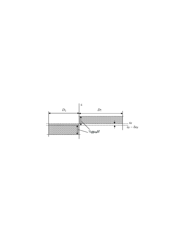
Figure 1: Redistribution of Fermi electrons to a shifted Fermi level $\varepsilon_{\mathrm{F}}-\delta\varepsilon_{\mathrm{F}}$, after Zeeman shifts of each spin subband.

This can be done, for instance, using the simplest two-subband Stoner model stoner for the total electronic energy:

$$E=\sum_{\mathbf{k},\sigma}\varepsilon_{\mathbf{k}}n_{\mathbf{k},\sigma}+Jn_{\uparrow}n_{\downarrow}-h\sum_{\sigma}\sigma n_{\sigma},$$ (2)

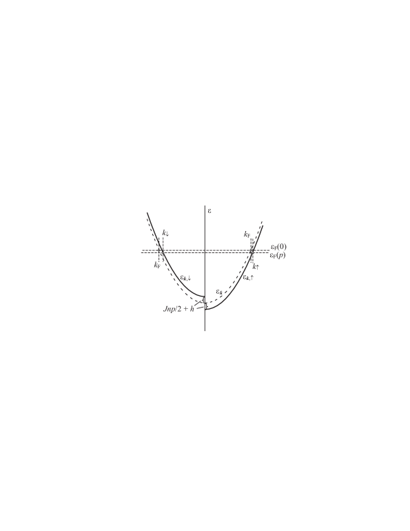
Figure 2: Band structure of a Stoner ferromagnet displaying shifted subbands $\varepsilon_{k,\sigma}$ and shifted Fermi level $\varepsilon_{{\textrm{F}}}\left(p\right)$ at finite polarization of subbands, compared to the paramagnetic values $\varepsilon_{k}$ and $\varepsilon_{{\textrm{F}}}\left(0\right)$. Vertical dashed lines show displaced limiting wavenumbers $k_{\uparrow,\downarrow}$ for spin subbands, compared to the paramagnetic value $k_{\textrm{F}}$.

where $n_{\mathbf{k},\sigma}$ is the occupation number for electronic state with momentum $\mathbf{k}$ and spin $\frac{1}{2}\sigma$ (in what follows $\uparrow$ is identified with $\sigma=1$ and $\downarrow$ with $\sigma=-1$), $n_{\sigma}=\sum_{\mathbf{k}}n_{\mathbf{k},\sigma}$ the partial electronic density, $\varepsilon_{\mathbf{k}}$ the paramagnetic dispersion law, $J$ the Stoner coupling constant, and $h=\frac{1}{2}g\mu_{{\textrm{B}}}H$ the Zeeman energy. The standard routine of this model is to minimize $E$ with respect to the band polarization $p=\left(n_{\uparrow}-n_{\downarrow}\right)/n$ (for given total electronic density $n=n_{\uparrow}+n_{\downarrow}$) and to obtain the equilibrium value of $p$, which can be field dependent: $p=p\left(h\right)$. But then we further use the obtained $p$ to calculate the shift of Fermi level $\varepsilon_{{\textrm{F}}}\left(p\right)$ vs its value in the paramagnetic state $\varepsilon_{\mathrm{F}}=\varepsilon_{\mathrm{F}}\left(0\right)$ (see Fig. 2).

For isotropic dispersion $\varepsilon_{\mathbf{k}}=\varepsilon_{k}$ and zero temperature, the occupation numbers are simply $n_{\mathbf{k},\sigma}=n_{k,\sigma}=\theta\left(k_{\sigma}-k\right)$, where the limiting wavenumber $k_{\sigma}$ can be expressed from the relation for the partial density:

$$n_{\sigma} = \sum_{k<k_{\sigma}}1\approx\frac{1}{2\pi^{2}}\int_{0}^{k_{\sigma}}k^{2}dk$$ (3)

$$= \frac{k_{\sigma}^{3}}{6\pi^{2}}=\frac{k_{\mathrm{F}}^{3}\left(1+\sigma p\right)}{6\pi^{2}},$$

through the paramagnetic $k_{\mathrm{F}}$ and $p$. Then the dispersion law for (polarized) $\sigma$th subband can be defined in accordance with the usual scheme of Landau Fermi liquid (LFL) theory:

$$\varepsilon_{k,\sigma}=\frac{\delta E}{\delta n_{k,\sigma}}=\varepsilon_{k}-\sigma\left(\frac{Jnp}{2}+h\right)+\rm{const},$$ (4)

where the $\sigma$-independent constant can be safely put zero. The uniform $\sigma$-dependent shift with respect to the paramagnetic dispersion $\varepsilon_{k}$ includes the two components of molecular field, the Stoner exchange field $Jnp/2$ and the external field $h$. The condition for unique Fermi level in both subbands reads

$$\varepsilon_{k_{\uparrow},\uparrow}=\varepsilon_{k_{\downarrow},\downarrow}=\varepsilon_{\mathrm{F}}\left(p\right),$$ (5)

and, evidently, the paramagnetic Fermi level is $\varepsilon_{\mathrm{F}}=\varepsilon_{k_{\mathrm{F}}}$. Then we present the total energy as

$$E=\sum_{\sigma}\sum_{k<k_{\sigma}}\varepsilon_{k}-np\left(\frac{Jp}{4}+h\right)+{\textrm{const}},$$

and, taking account of Eq. 3 and using the parabolic dispersion $\varepsilon_{k}\propto k^{2}$, obtain its explicit dependence on $p$:

$$E\left(p\right) = n\left\{\frac{3\varepsilon_{{\textrm{F}}}}{10}\left[\left(1+p\right)^{5/3}+\left(1-p\right)^{5/3}\right]\right.$$ (6)

$$\qquad\qquad\qquad\qquad\left.-p\left(\frac{Jp}{4}+h\right)\right\}.$$

The necessary minimum condition for Eq. 6:

$$\varepsilon_{{\textrm{F}}}\left[\left(1+p\right)^{2/3}-\left(1-p\right)^{2/3}\right]=2\left(\frac{Jnp}{2}+h\right),$$

is just equivalent to Eq. 5, and, being expanded for small polarization $p\ll 1$ and weak external field $h\ll Jnp$, leads to

$$p\left(h\right)\approx p\left(0\right)+\frac{27h}{8\varepsilon_{{\textrm{F}}}p^{2}\left(0\right)},$$ (7)

where the spontaneous polarization

$$p\left(0\right)=3\sqrt{\frac{1}{2}\left(\frac{3Jn}{4\varepsilon_{{\textrm{F}}}}-1\right)}=3\sqrt{\frac{1}{2}\left(JD_{\mathrm{F}}-1\right)}$$

includes the paramagnetic Fermi density of states $D_{\mathrm{F}}\approx\left(D_{\uparrow}+D_{\downarrow}\right)/2$. Finally, substituting Eq. 7 into Eqs. 5 and 4 results in the sought expression for shifted Fermi level:

$$\varepsilon_{{\textrm{F}}}\left(p\right)\approx\varepsilon_{{\textrm{F}}}\left(0\right)\left[1-\frac{p^{2}\left(0\right)}{9}\right]-\frac{3h}{4p\left(0\right)}.$$ (8)

This formula indicates that the sharpest response of $\varepsilon_{{\textrm{F}}}$ to external field (when small enough: $h\ll\varepsilon_{{\textrm{F}}}p^{3}\left(0\right)$) is achieved with the lowest band polarization $p\left(0\right)$, that is close to the Stoner critical condition: $JD_{\mathrm{F}}\approx 1$. In this case, the $h$-dependent contribution to $Jnp/2$ from the second term in r.h.s. of Eq. 7 is $\approx h(3/2p(0))^{2}\gg h$, that is dominating over the proper Zeeman term $h$ in the molecular field $Jnp/2+h$, which defines a great difference with the Ono et al result. This can be expected, considering the LFL relation $\varepsilon_{{\textrm{F}}}=\delta E/\delta n$ and the phenomenological dependence of total energy on external field $E=E_{H=0}-\chi H^{2}$ with the mean-field behavior of susceptibility $\chi\sim 1/p(0)$. We also notice that the band polarization $p$ in Eq. 8 is quite different from the Fermi level polarization $P$ in Eq. 1, and (for non-parabolic dispersion) can even have opposite sign. Practically, the required closeness to critical condition can be met in various transition metal alloys, as e.g. Pd-Fe, Rh-Fe, or Ru-Co, though, when passing from bulk material to nanoparticles, the particular compositions of these systems might need to be reconsidered.

Since the Stoner critical point corresponds to a kind of quantum phase transitions sachdev , kirk , an important question is the possible effect of quantum critical fluctuations which can put some restrictions on the choice of operating parameters. In particular, the correlation length of quantum fluctuations is estimated as $\xi_{c}\sim ak_{\mathrm{B}}T_{c}/(\varepsilon_{\mathrm{F}}p(0))$ where $a$ is interatomic distance, $k_{\mathrm{B}}$ the Boltzmann constant, $T_{c}$ the characteristic temperature of magnetic ordering in the saturated state (far from the quantum critical point), and in order that fluctuations stay smaller of the nanoparticle size $d$ one needs the spontaneous polarization no less then $p_{min}\sim ak_{\mathrm{B}}T_{c}/(d\varepsilon_{\mathrm{F}})$. Then, with typical values $a\sim 0.3$ nm, $T_{c}\sim 300$ K, $d\sim 5nm$, $\varepsilon_{\mathrm{F}}\sim 1$ eV we obtain $p_{min}\sim 10^{-3}$, permitting a really high enhancement by Eq. 8.

An additional enhancement of the field response of the N-I-M-I-N device can be found, considering Coulomb blocade and Coulomb staircase effects at tunneling through nanoparticles shimada ,ono ,imamura , so that the system can be previously driven by a common gate bias to the point of steepest $dI/dV$ and then used to detect the current variation due to weak magnetic signal $\delta h$:

$$\delta I=\frac{3\delta h}{4p\left(0\right)}\frac{dI}{dV}.$$

In conclusion, the simple analysis based on two-subband Stoner model for total electronic energy shows that an effective control of tunnel conductance can be achieved by tuning the position of Fermi level in one of the electrodes with relatively weak external magnetic field. This tuning is most pronounced when the material of the considered electrode is chosen to be close to the Stoner critical condition for ferromagnetic transition. The extension of this model to more realistic band structures and exchange coupling schemes marcus is straightforward. The proposed magnetic tuning mode can open a new route for modern spintronic devices.

References

- (1) S.A. Wolf, D.D. Awschalom, R.A. Buhrmann, R.A. Daughton, S. von Molnar, M.L. Roukes, A.Y. Chtchelkanova, and D.M. Treger, Science 294, 1488 (2001).
- (2) S. Das Sarma, J. Fabian, X. Hu, I. Zutic, IEEE Trans. Magn. 36, 2821 (2000).
- (3) T. Miyazaki and N. Tezuka, J. Magn. Magn. Mater. 139, L231 (1995).
- (4) J.S. Moodera, L.R. Kinder, T.M. Wong, and R. Meservey, Phys. Rev. Lett. 74, 3273 (1995).
- (5) M. Julliere, Phys. Lett. 54A, 225 (1975).
- (6) H. Shimada, K. Ono, and Y. Ootuka, J. Phys. Soc. Japan 67, 1359 (1998).
- (7) K. Ono, H. Shimada, and Y. Ootuka, J. Phys. Soc. Japan 67, 2852 (1998).
- (8) E.C. Stoner, Proc. Roy. Soc. London, Ser. A 165, 372 (1938).
- (9) S. Sachdev, “Quantum Phase Transitions”, Cambridge University Press, Cambridge (1999).
- (10) T.R. Kirkpatrick and D. Belitz, in “Electron Correlation in Solid State”, ed. Norman H. March, Imperial College Press, London (1999), pp. 297-370.
- (11) H. Imamura, J. Chiba, S. Mitani, K. Takanashi, S. Takahashi, S. Maekawa, H. Fujimori, Phys. Rev. B61, 46 (2000).
- (12) P.M. Marcus, V.L. Moruzzi, Phys. Rev. B 38, 6949 (1988).