Quantum oscillations in mesoscopic rings and anomalous diffusion

Abstract

We consider the weak localization correction to the conductance of a ring connected to a network. We analyze the harmonics content of the Al’tshuler-Aronov-Spivak (AAS) oscillations and we show that the presence of wires connected to the ring is responsible for a behaviour different from the one predicted by AAS. The physical origin of this behaviour is the anomalous diffusion of Brownian trajectories around the ring, due to the diffusion in the wires. We show that this problem is related to the anomalous diffusion along the skeleton of a comb. We study in detail the winding properties of Brownian curves around a ring connected to an arbitrary network. Our analysis is based on the spectral determinant and on the introduction of an effective perimeter probing the different time scales. A general expression of this length is derived for arbitrary networks. More specifically we consider the case of a ring connected to wires, to a square network, and to a Bethe lattice.

^(a)Laboratoire de Physique Théorique et Modèles Statistiques, associé au CNRS, Bât. 100,
^(b)Laboratoire de Physique des Solides, associé au CNRS, Bât. 510,
  Université Paris-Sud, F-91405 Orsay cedex, France.

PACS numbers : 73.23.-b ; 73.20.Fz ; 72.15.Rn ; 02.50.-r ; 05.40.Jc.

1 Introduction

At a classical level, a network made of diffusive wires can be described as an ensemble of classical resistances. Quantum corrections bring a small sample specific contribution whose disorder average is called the weak localization (WL) correction. This contribution is sensitive to a magnetic field and makes the average conductivity of a phase coherent ring be a periodic function of the magnetic flux $\phi$ through the ring with periodicity $\phi_{0}/2$, where $\phi_{0}=h/e$ is the flux quantum. This is the so-called Al’tshuler-Aronov-Spivak (AAS) effect [1]. The case of an isolated ring was considered by AAS who showed that the average correction to the classical conductivity varies as :

$$\Delta\sigma(\theta)=-\frac{e^{2}}{h}L_{\varphi}\frac{\sinh(L/L_{\varphi})}{\cosh(L/L_{\varphi})-\cos(\theta)}$$ (1)

where $L$ is the perimeter and $\theta=4\pi\phi/\phi_{0}$ the reduced flux. Phase breaking mechanisms are taken into account through the characteristic length $L_{\varphi}$ called the phase coherence length. The harmonics of the oscillations

$$\Delta\sigma^{(n)}=\int_{0}^{2\pi}\frac{{\rm d}\theta}{2\pi}\Delta\sigma(\theta)\>{\mbox{\large e}}^{-{\rm i}n\theta}=-\frac{e^{2}}{h}L_{\varphi}\>{\mbox{\large e}}^{-|n|L/L_{\varphi}}$$ (2)

decay exponentially with the perimeter $L$ of the ring and the order $n$ of the harmonic. The relation (2) was derived for an isolated ring and it is not clear, when studying the transport through a ring connected by wires to reservoirs, how this correction to the conductivity is related to the correction to the conductance. Moreover the presence of the connecting wires can seriously modify the harmonics content of the AAS oscillations. In this paper we show that, if the perimeter $L$ of the ring is much smaller than $L_{\varphi}$ and if the connecting wires are much longer than $L_{\varphi}$, the $n$th harmonic decreases like $\exp-n\sqrt{N_{a}L/L_{\varphi}}$, that is faster than (2). $N_{a}$ is the number of wires attached to the ring.

The paper is organized as follows : in section 2 we briefly recall the general expression of the WL correction on a network and we present some results for the conductance through a connected ring. The rest of the paper is devoted to the analysis of the new behaviour of the harmonics. This is achieved by studying in detail the winding properties of Brownian curves around a ring connected to a network. In section 3 we present our general method, based on the spectral determinant which encodes the necessary information on the network. In section 4 we consider specifically the question of a ring connected to one or several wires. We show that the new behaviour $\exp-n\sqrt{N_{a}L/L_{\varphi}}$ is the signature of an anomalous diffusion around the ring. In section 5 we study the case where the ring is connected to an arbitrary network. We relate the winding properties around the ring to the recurrent character of the Brownian motion in the network.

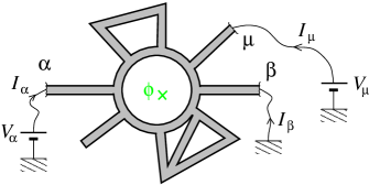
Figure 1: A network connected to reservoirs and pierced by a magnetic flux $\phi$. The wavy lines represent connection to large contacts (external reservoirs).

2 Quantum transport through a connected ring

Recently, we have obtained a general expression for the weak localization (WL) correction on a network [2, 3]. Let us remind first how it reads for a wire. The classical conductance of a wire of section $s$ and length $L$ is given by the Ohm’s law $G^{\rm cl}=\sigma_{0}s/L$ where $\sigma_{0}$ is the Drude conductivity. This result can be rewritten in terms of the total transmission through the wire, i.e. the dimensionless conductance, $T^{\rm cl}_{\rm wire}=\alpha_{d}N_{c}\ell_{e}/L$, where $N_{c}$ is the number of channels, $\ell_{e}$ the elastic mean free path and $\alpha_{d}$ a numerical constant depending on the dimension ($\alpha_{1}=2$, $\alpha_{2}=\pi/2$ and $\alpha_{3}=4/3$). The interferences between reversed trajectories are described by the so-called cooperon $P_{c}(x,x)$ which measures the return probability for a diffusive particle and which is solution of a diffusion equation that we will recall in section 3. These interferences give rise to the WL correction which is expressed as

$$\Delta T_{\rm wire}=-\frac{2}{L^{2}}\int_{0}^{L}{\rm d}x\,P_{c}(x,x)\>.$$ (3)

More generally, for a network attached to leads $\alpha$ and $\beta$ as shown on figure 1, the classical transmission coefficient is obtained by classical Kirchhoff laws and it has the form $T^{\rm cl}_{\alpha\beta}=\alpha_{d}N_{c}\ell_{e}/{\cal L}_{\alpha\beta}$ where the equivalent length ${\cal L}_{\alpha\beta}$ is function of the lengths of the wires, the topology of the network and the way it is connected to external reservoirs. Note that ${\cal L}_{\alpha\beta}$ is simply proportional to the equivalent resistance.

On such a network, because of the absence of translation invariance, we have shown recently that the cooperon must be properly weighted when integrated over the wires of the networks to get the WL correction to the transmission coefficient. Equation (3) generalizes as [2] :

$$\Delta T_{\alpha\beta}=\frac{2}{\alpha_{d}N_{c}\ell_{e}}\sum_{(\mu\nu)}\frac{\partial T^{\rm cl}_{\alpha\beta}}{\partial\,l_{\mu\nu}}\int_{(\mu\nu)}{\rm d}x\,P_{c}(x,x)\>.$$ (4)

The sum runs over all wires $(\mu\nu)$ of the network. The cooperon is integrated over each wire $(\mu\nu)$, with a weight which is simply the derivative of the classical transmission with respect to its length $l_{\mu\nu}$. This WL correction depends on the lengths of the wires, the phase coherence length $L_{\varphi}$, the magnetic field and the topology of the network.

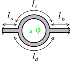
Figure 2: A mesoscopic ring connected at two reservoirs.

We consider the transport through the ring of figure 2. The classical transmission reads $T^{\rm cl}_{\rm ring}=\frac{\alpha_{d}N_{c}\ell_{e}}{l_{a}+l_{c/\!/d}+l_{b}}$, where $l_{c/\!/d}^{-1}=l_{c}^{-1}+l_{d}^{-1}$. To simplify the calculations we consider below the symmetric case $l_{a}=l_{b}$ and $l_{c}=l_{d}=L/2$. The calculation of the WL correction $\Delta T_{\rm ring}(\theta)$, given by (4), requires the construction of the cooperon in the network, explained in [2, 3]. We do not give further details nor the full result [3] and we only present two limiting cases for the Fourier decomposition $\Delta T_{\rm ring}^{(n)}~{}$:

$\bullet$ The weakly coherent network $L_{\varphi}\ll L,l_{a}$.

$$\Delta T_{\rm ring}^{(n)}\simeq-\frac{L\,L_{\varphi}}{4(2l_{a}+L/4)^{2}}\left(\frac{2}{3}\right)^{2n}{\mbox{\large e}}^{-n\,L/L_{\varphi}}\hskip 14.22636pt\mbox{ for }n>0\>.$$ (5)

We get an exponential behaviour coinciding with the one predicted by AAS. The factor $\left({2}/{3}\right)^{2n}$ is related to the probability to cross $2n$ times a vertex of coordinence 3 [7]. This result shows that the connecting wires play an important role and that the determination of $L_{\varphi}$ from ratio of harmonics using formula (2) can lead to a wrong estimate.

$\bullet$ The mesoscopic ring connected to long wires $L\ll L_{\varphi}\ll l_{a}$.

$$\Delta T_{\rm ring}^{(n)}\simeq-\left(\frac{L_{\varphi}}{2l_{a}}\right)^{2}\sqrt{\frac{L}{2L_{\varphi}}}\>{\mbox{\large e}}^{-n\,\sqrt{2L/L_{\varphi}}}\hskip 14.22636pt\mbox{ for }n>0\>.$$ (6)

The harmonics decay presents a strikingly different behaviour from the one given by AAS. This can be understood in the following way : because $L\ll L_{\varphi}$, whenever a diffusive trajectory encircles the ring, it explores a distance in the arm which can be much longer than the perimeter of the ring. This leads to an effective perimeter $L_{\rm eff}\simeq\sqrt{2L_{\varphi}L}\gg L$ which is responsible for a decrease of the harmonics with $n$ faster than (2). In the next sections, we examine in detail the effect of the arms on the winding properties around the loop in order to analyze the origin of the new behaviour (6).

3 Winding of Brownian trajectories and spectral determinant

In this section, we recall how the harmonics of the WL correction, $\Delta T^{(n)}_{\rm ring}$, can be related to the winding properties of diffusive trajectories around the ring. For this purpose we introduce the probability to start from a point $x$ and come back to it after a time $t$ having performed $n$ windings around the loop. This probability can be written with a path integral as :

$$W_{n}(x,x;t)=\int_{x(0)=x}^{x(t)=x}{\cal D}x(\tau)\>{\mbox{\large e}}^{-\frac{1}{4}\int_{0}^{t}{\rm d}\tau\,\dot{x}(\tau)^{2}}\delta_{n,{\cal N}[x(\tau)]}$$ (7)

where ${\cal N}[x(\tau)]=\int_{0}^{t}{\rm d}\tau\,\dot{x}(\tau)$ is the winding number of the diffusive trajectory $x(\tau)$. We have chosen a diffusion constant equal to unity $D=1$. If we write $\delta_{n,{\cal N}}=\int_{0}^{2\pi}\frac{{\rm d}\theta}{2\pi}{\mbox{\large e}}^{{\rm i}({\cal N}-n)\theta}$, the coupling of the winding number to the conjugate parameter $\theta$ in the action is interpreted as the coupling to a magnetic flux. The Laplace transform with respect to time relates the probability $W_{n}(x,x;t)$ to the cooperon $P_{c}(x,x)$ :

$$\int_{0}^{\infty}{\rm d}t\,W_{n}(x,x;t)\,{\mbox{\large e}}^{-\gamma t} = \int_{0}^{2\pi}\frac{{\rm d}\theta}{2\pi}{\mbox{\large e}}^{-{\rm i}n\theta}\int_{0}^{\infty}{\rm d}t\,{\mbox{\large e}}^{-\gamma t}\int_{x(0)=x}^{x(t)=x}{\cal D}x\>{\mbox{\large e}}^{-\frac{1}{4}\int_{0}^{t}{\rm d}\tau\,\dot{x}^{2}+{\rm i}\frac{\theta}{L}\int_{0}^{t}{\rm d}\tau\,\dot{x}}$$ (8)

$$= \int_{0}^{2\pi}\frac{{\rm d}\theta}{2\pi}\>{\mbox{\large e}}^{-{\rm i}n\theta}\>P_{c}(x,x)\>.$$ (9)

The cooperon $P_{c}(x,x^{\prime})$ is solution of a diffusion-like equation $[\gamma-{\rm D}_{x}^{2}]P_{c}(x,x^{\prime})=\delta(x-x^{\prime})$ where the covariant derivative is ${\rm D}_{x}=\frac{{\rm d}}{{\rm d}x}-{\rm i}A(x)$ with $A(x)=\theta/L$ for $x$ inside the ring. In the WL theory, the cooperon describes the contribution of quantum interferences, that are limited by phase breaking mechanisms. In this respect, the Laplace parameter $\gamma$ plays the role of a phenomenological parameter that selects the diffusive trajectories for times $t<1/\gamma$. This parameter is related to the phase coherence length $L_{\varphi}$, that gives the length scale over which quantum interferences can occur, by $\gamma=1/L_{\varphi}^{2}$. The $n$-th harmonics of the WL correction $\Delta T_{\rm ring}^{(n)}$ is given by an integral over $x$ of the Laplace transform $\int_{0}^{\infty}{\rm d}t\,W_{n}(x,x;t)\,{\mbox{\large e}}^{-\gamma t}$. The integration over the network is performed by weighting the wires with the coefficients given in eq. (4).

The relation between WL and properties of the Brownian motion was formulated in other works like [4, 5].

3.1 Probability averaged over the network

First, we do not consider the dependence on the initial point $x$ and average over it. We define $W_{n}(t)=\int{\rm d}x\,W_{n}(x,x;t)$. In order to study this quantity it is useful to introduce the spectral determinant, defined as $S(\gamma)=\prod_{n}(\gamma+E_{n}(\theta))$, where $\{E_{n}(\theta)\}$ is the spectrum of the operator $-{\rm D}_{x}^{2}$. The spectral determinant is related to the cooperon in the following way : $\int{\rm d}x\,P_{c}(x,x)={\rm Tr}\{\frac{1}{\gamma-{\rm D}_{x}^{2}}\}=\sum_{n}\frac{1}{\gamma+E_{n}}=\frac{\partial}{\partial\gamma}\ln S(\gamma)$. Therefore the probability $W_{n}(t)$ can be conveniently written as :

$$\int_{0}^{\infty}{\rm d}t\,W_{n}(t)\,{\mbox{\large e}}^{-\gamma t}=\int_{0}^{2\pi}\frac{{\rm d}\theta}{2\pi}\>{\mbox{\large e}}^{-{\rm i}n\theta}\frac{\partial}{\partial\gamma}\ln S(\gamma)\>.$$ (10)

The interest to introduce the spectral determinant is that it is a global quantity encoding all informations about the spectrum. This approach is especially efficient for networks thanks to the compact expression of $S(\gamma)$ obtained in [6] : it can be related to the determinant of a finite size matrix that encodes the information on the topology of the networks, the lengths of the wires, the magnetic fluxes and the way the network is connected to external reservoirs. This relation is briefly recalled in the appendix A.

3.2 Probability for a fixed initial condition

It is also interesting to study the probability $W_{n}(x_{0},x_{0};t)$ for $n$ windings in a time $t$ when the initial condition $x_{0}$ is fixed. This requires some local information which is obtained from the construction of $P_{c}(x_{0},x_{0})$ inside the network (the expression can be found in [3]). We propose here a method to obtain this local information still using the spectral determinant. This latter encodes a global information since it results from a spatial integration of the cooperon over the network. It is related to a sum over the eigenvalues of the Laplace operator $\sum_{n}\frac{1}{\gamma+E_{n}}$. On the other hand $P_{c}(x_{0},x_{0})$ requires some local information on the eigenfunctions. In order to extract this local information we introduce the modified cooperon $P_{c}^{(\lambda_{0})}$, solution of $[\gamma-{\rm D}_{x}^{2}+\lambda_{0}\delta(x-x_{0})]P_{c}^{(\lambda_{0})}(x,x^{\prime})=\delta(x-x^{\prime})$. The corresponding spectral determinant is $\partial_{\gamma}\ln S^{(\lambda_{0})}(\gamma)=\int{\rm d}x\,P_{c}^{(\lambda_{0})}(x,x)$. Its expansion in powers of the parameter $\lambda_{0}$ leads to : $\partial_{\gamma}\ln S^{(\lambda_{0})}(\gamma)=\partial_{\gamma}\ln S(\gamma)+\lambda_{0}\partial_{\gamma}P_{c}(x_{0},x_{0})+O(\lambda_{0}^{2})$. The cooperon at $x_{0}$ can be obtained by computing the spectral determinant $S^{(\lambda_{0})}(\gamma)$ for a $\delta$ added at $x_{0}$ :

$$P_{c}(x_{0},x_{0})=\frac{{\rm d}}{{\rm d}\lambda_{0}}\ln S^{(\lambda_{0})}(\gamma)\Big{|}_{\lambda_{0}=0}\>,$$ (11)

and inserted in (9). For a network, the computation of $S^{(\lambda_{0})}(\gamma)$ is especially simple : $\lambda_{0}$ is interpreted as the parameter involved in the boundary condition at a vertex at $x_{0}$ (see appendix A).

4 Winding around a ring with an arm

In this section we study how the winding properties inside a ring are affected by the presence of an arm. We first recall the simple case of the isolated ring and consider the case of the ring with one arm (figure 3a) for different kinds of boundary conditions at the end of the arm.

4.1 Spectral determinant and winding properties

A reminder : the isolated ring.– In order to illustrate our formalism, we start by recalling few simple results about the isolated ring, that will be useful for the following. The quantity at the basis of our analysis is the spectral determinant, that reads for the isolated ring : $S(\gamma)=2(\cosh\sqrt{\gamma}L-\cos\theta)$. The relation (10) shows that the Laplace transform of the probability $W_{n}(t)$ require a Fourier transform of $\frac{\partial}{\partial\gamma}\ln S(\gamma)=\frac{L}{2\sqrt{\gamma}}\frac{\sinh\sqrt{\gamma}L}{\cosh\sqrt{\gamma}L-\cos\theta}$. We obtain

$$\int_{0}^{\infty}{\rm d}t\,W_{n}(t)\,{\mbox{\large e}}^{-\gamma t}=\frac{L}{2\sqrt{\gamma}}{\mbox{\large e}}^{-n\sqrt{\gamma}L}\>,$$ (12)

which is the exponential behaviour recalled in eq. (2). It is worth noticing that the translation invariance of the system implies that $W_{n}(t)=LW_{n}(x,x;t)$. The inverse Laplace transform leads to

$$W_{n}(x,x;t)=\frac{1}{2\sqrt{\pi t}}{\mbox{\large e}}^{-\frac{(nL)^{2}}{4t}}$$ (13)

which characterizes normal diffusion in the ring. We can study the scaling of the winding number with time by computing $n_{t}=\sqrt{\langle n^{2}\rangle_{t}}$, where $\langle\cdots\rangle_{t}$ denotes averaging over all trajectories for a time $t$. The ring possesses a characteristic time scale : the Thouless time. In units such that $D=1$, it reads $\tau_{L}=L^{2}$. It is the time needed by a diffusive trajectory to explore the ring. In the short time limit $t\ll\tau_{L}$, we obtain $n_{t}\simeq\sqrt{2}\exp-\frac{L^{2}}{8t}$ and in the long time limit $t\gg\tau_{L}$ we get $n_{t}\simeq\sqrt{2}\,t^{1/2}/L$.

Figure 3: Left : A network with one loop and one arm. A general boundary condition ($\lambda_{1}$) is chosen at vertex 1. $\lambda_{1}=0$ describes a reflecting boundary (isolated network). $\lambda_{1}=\infty$ descibes an absorbing boundary (connection to a reservoir). Right : The study of the winding in the ring is equivalent to study the displacement along the skeleton of a comb.

Dirichlet boundary at the end of the arm.– We now consider the winding in a ring with an arm. A Dirichlet boundary at the end of the wire describes absorption (connection to a reservoir). In terms of the parameter introduced in the appendix A, this corresponds to $\lambda_{1}=\infty$. The spectral determinant of the ring of figure 3a is easily obtained (see [6, 7, 3] and appendix A). It presents a structure similar to the one of the isolated ring,

$$\sqrt{\gamma}S_{\rm Dir}(\gamma)=2\sinh\sqrt{\gamma}b\,\left[\cosh\sqrt{\gamma}L_{\rm eff}^{\rm Dir}-\cos\theta\right]\>,$$ (14)

where we have introduced $L_{\rm eff}^{\rm Dir}$, defined by

$$\cosh\sqrt{\gamma}L_{\rm eff}^{\rm Dir}=\cosh\sqrt{\gamma}L+\frac{1}{2}\sinh\sqrt{\gamma}L\,\coth\sqrt{\gamma}b\>.$$ (15)

Interestingly, the flux dependance $S(\gamma)\propto\cosh\sqrt{\gamma}L_{\rm eff}-\cos\theta$ immediatly leads to the behaviour $\int_{0}^{\infty}{\rm d}t\,W_{n}(t)\,{\mbox{\large e}}^{-\gamma t}\propto{\mbox{\large e}}^{-n\sqrt{\gamma}L_{\rm eff}}$. In general the length $L_{\rm eff}$ depends on $\gamma$. Since $\gamma$ is the parameter conjugate to the time $t$, it probes times $t\sim 1/\gamma$. Therefore $L_{\rm eff}(\gamma)$ is the effective perimeter for winding trajectories at a time scale $t=1/\gamma$.

In the limit $b\to 0$ the spectral determinant becomes $S_{\rm Dir}(\gamma)|_{b=0}=\sinh\sqrt{\gamma}L/\sqrt{\gamma}$ which is the result for a wire with Dirichlet boundary at its ends. The reservoir acting as a phase breaker, the phase sensitivity is lost since the reservoir is now located in the ring.

Neumann boundary at the end of the arm.– It is also interesting to study the spectral determinant for Neumann boundary at the end of the arm, $\lambda_{1}=0$, which describes a reflection of the diffusive particle (isolated network). In this case [7]

$$S_{\rm Neu}(\gamma)=2\cosh\sqrt{\gamma}b\,\left[\cosh\sqrt{\gamma}L_{\rm eff}^{\rm Neu}-\cos\theta\right]$$ (16)

where the effective perimeter now reads

$$\cosh\sqrt{\gamma}L_{\rm eff}^{\rm Neu}=\cosh\sqrt{\gamma}L+\frac{1}{2}\sinh\sqrt{\gamma}L\,\tanh\sqrt{\gamma}b\>.$$ (17)

In this case the limit $b\to 0$ leads to the spectral determinant of an isolated ring $S_{\rm Neu}(\gamma)|_{b=0}=2(\cosh\sqrt{\gamma}L-\cos\theta)$.

We now analyze the different behaviours in a time representation to understand their physical significance in the diffusion problem. To analyze the diffusion at time $t$, we have to consider $\gamma=1/t$. In the following we keep using the notation $\gamma=1/L_{\varphi}^{2}$ for convenience. In addition to the Thouless time $\tau_{L}=L^{2}$ needed to explore the ring, there is a second characteristic time $\tau_{b}=b^{2}$ which is the typical time required to explore the arm.

$\bullet$ Short times $t\ll\tau_{L},\tau_{b}$ (i.e. $L_{\varphi}\ll L,b$).– In this case the arm is explored over a distance smaller than the perimeter and the presence of the arm has a small influence. The precise nature of the boundary condition is not felt when diffusing inside the loop, since the trajectories encircling the loop do not have enough time to reach the end of the arm ($t\ll\tau_{b}$). This is reflected by the fact that $L_{\rm eff}^{\rm Dir}=L_{\rm eff}^{\rm Neu}$ in this limit. From the expressions (15,17), we obtain the effective parameter $L_{\rm eff}\simeq L+L_{\varphi}\ln(3/2)$. We recover the behaviour of the isolated ring $n_{t}\simeq\sqrt{2}\exp-\frac{L^{2}}{8t}$.

$\bullet$ Intermediate times $\tau_{L}\ll t\ll\tau_{b}$ (i.e. $L\ll L_{\varphi}\ll b$).– The particle can turn diffusively many times around the loop but cannot explore the arm up to its end. This is a limit of an infinitely long arm. Like in the previous case, the boundary condition plays no role. From (15,17), the effective length is $L_{\rm eff}\simeq\sqrt{L}\,\gamma^{-1/4}=\sqrt{LL_{\varphi}}$. By using (10) we obtain :

$$\int_{0}^{\infty}{\rm d}t\,W_{n}(t)\,{\mbox{\large e}}^{-\gamma t}\simeq\frac{\sqrt{L}}{4\gamma^{3/4}}\,{\mbox{\large e}}^{-n\sqrt{L}\,\gamma^{1/4}}\>,$$ (18)

which leads to the harmonic content (6) . The inverse Laplace transform gives

$$W_{n}(t)=\theta(t)\frac{\sqrt{L}}{4\,t^{1/4}}\ \chi\!\left(\xi=\frac{n\sqrt{L}}{t^{1/4}}\right)$$ (19)

where $\chi(\xi)=\frac{4}{\pi}\int_{0}^{\infty}{\rm d}u\,{\mbox{\large e}}^{-u^{4}-\frac{1}{\sqrt{2}}\xi u}\cos\left(\frac{1}{\sqrt{2}}\xi u+\frac{\pi}{4}\right)=\frac{4}{\pi}\mathop{\mathrm{Re}}\nolimits({\mbox{\large e}}^{{\rm i}\frac{\pi}{4}}\int_{0}^{\infty}{\rm d}u\,{\mbox{\large e}}^{-\varphi(u)})$ with $\varphi(u)=u^{4}+u\,\xi\,{\mbox{\large e}}^{-{\rm i}\frac{\pi}{4}}$. $\theta(t)$ is the Heaviside function. The function at the origin is $\chi(0)=\frac{\Gamma(1/4)}{\pi\sqrt{2}}$ while it presents an exponential tail :

$$\chi(\xi)\simeq\frac{4}{\sqrt{6\pi}}\>\frac{1}{\left(\xi/4\right)^{1/3}}\,{{\mbox{\large e}}^{-3\,({\xi}/{4})^{4/3}}}\hskip 7.11317pt\mbox{for }\xi\gg 1\>.$$ (20)

As a result, the tail of the distribution behaves like

$$W_{n}(t)\sim\frac{1}{t^{1/6}n^{1/3}}\exp{-c\frac{n^{4/3}}{t^{1/3}}}\>,$$ (21)

where $c$ is a coefficient. We will see in section 4.4 that for a fixed initial condition $W_{n}(x,x;t)$ presents the same exponential behaviour with a different prefactor. This expression shows that the winding number scales like $n_{t}\propto t^{1/4}$.

$\bullet$ Large times $\tau_{L},\tau_{b}\ll t$ (i.e. $L,b\ll L_{\varphi}$).– In this regime the diffusive trajectories can explore the arm until its end and the precise nature of boundary condition matters.

For Neumann boundary condition, the expansion of (17) gives $L_{\rm eff}^{\rm Neu}\simeq\sqrt{L(L+b)}$. It is interesting to point that since the arm is explored until its end, this result can be simply obtained by replacing $L_{\varphi}$ by $L+b$ in the result $L_{\rm eff}\simeq\sqrt{LL_{\varphi}}$ obtained for $L\ll L_{\varphi}\ll b$. Since this effective perimeter does not depend on $\gamma$, it describes normal diffusion around the ring. However the diffusion constant is reduced due to the time spent in the arm $n_{t}\simeq\sqrt{2}\,t^{1/2}/\sqrt{L^{2}+bL}$.

For Dirichlet boundary, from (15), the effective length reads $L_{\rm eff}^{\rm Dir}\simeq L_{\varphi}\sqrt{L/b}$. This reflects a behaviour $\int_{0}^{\infty}{\rm d}t\,{\mbox{\large e}}^{-\gamma t}W_{n}(t)\propto{\mbox{\large e}}^{-n\sqrt{L/b}}$ independent on $\gamma$ which originates from the absorption at vertex $1$. The winding number reaches a finite value at infinite time : $n_{t}\simeq\sqrt{2b/L}$.

We summarize these results in table 1.

4.2 Relation with the anomalous diffusion along the skeleton of a comb

We discuss specifically the regime $\tau_{L}\ll t\ll\tau_{b}$ of an infinitely long arm. From (19) we have seen that the winding number scales with the time like

$$n_{t}\propto t^{1/4}\>.$$ (22)

The prefactor can be obtained from the method explained in the appendix B. We recall that the winding in a ring without arm (normal diffusion) is $n_{t}\simeq\sqrt{2}\,t^{1/2}/L$. In the presence of the arm, the Brownian trajectories can explore the arm over long distance when turning around the ring. For a time scale $t$ the effective perimeter of winding trajectories is $L_{\rm eff}(\gamma=1/t)\simeq\sqrt{L}\,t^{1/4}$. From this simple heuristic argument we recover the subdiffusive behaviour $n_{t}\sim t^{1/2}/L_{\rm eff}\sim t^{1/4}/\sqrt{L}$. We stress that “subdiffusion” refers to the time dependence of the winding number around the flux, and not to the motion inside the wires which obeys normal diffusion.

This problem is similar to the known problem of the diffusion along the skeleton of a comb : the diffusion in the ring is the periodisation of the diffusion along the skeleton of the comb (see figure 3). This problem has been studied by a different method in refs. [8] and [9] (note that the reference [9] corrected a wrong assumption about the nature of the distribution made in [8]), however the power law in front of the exponential was not given. The problem of diffusion along the skeleton of a comb belongs to a broader class of problems : the diffusion of a particle along a line with an arbitrary distribution of the waiting time $\tau$ spent on each site. It was shown that if the distribution of the waiting time presents an algebraic tail $P_{1}(\tau)\propto\tau^{-1-\mu}$ with $0<\mu<1$, the diffusion is subdiffusive with $n_{t}\sim t^{\mu/2}$ [10]. In the case of the diffusion in the comb, the distribution of the trapping time by the arm is given by the first return probability for the one-dimensional diffusion : $P_{1}(\tau)\propto\tau^{-3/2}$ and we recover $n_{t}\sim t^{1/4}$.

4.3 The case of $N_{a}$ arms

By using the mapping between the diffusion inside the ring and in the comb we immediately get the result for $N_{a}$ arms : the trajectory encounters $N_{a}$ arms for one turn, which corresponds to $N_{a}$ steps of length $L/N_{a}$ in the comb. Then the result for $N_{a}$ arms is obtained by a substitution $n\to nN_{a}$ and $L\to L/N_{a}$ which leads to $\int_{0}^{\infty}{\rm d}t\,W_{n}(t)\,{\mbox{\large e}}^{-\gamma t}\simeq\frac{\sqrt{L/N_{a}}}{4\gamma^{3/4}}\,{\mbox{\large e}}^{-n\sqrt{N_{a}L}\,\gamma^{1/4}}$. For $N_{a}=2$ the exponential dependence agrees with (6).

$\bullet$ $N_{a}$ arms attached regularly.– The result given by the previous simple argument can also be obtained from a calculation of $S(\gamma)$ for several arms. If $N_{a}$ arms of length $b$ are attached regularly around the ring we obtain

$$S(\gamma)=\left(\frac{2\sinh\sqrt{\gamma}b}{\sqrt{\gamma}}\right)^{N_{a}}\prod_{n=1}^{N_{a}}\left[\cosh(\frac{\sqrt{\gamma}L}{N_{a}})-\cos(\frac{2\pi n+\theta}{N_{a}})+\frac{1}{2}\sinh(\frac{\sqrt{\gamma}L}{N_{a}})\coth\sqrt{\gamma}b\right]$$ (23)

for Dirichlet boundary conditions at the end of the arms. For $N_{a}=1$ we recover (14). (The spectral determinant for Neumann boundary conditions is given in chapter 5 of [11]). For short times, $t\ll\tau_{L},\tau_{b}$, we get $L_{\rm eff}\simeq L+N_{a}L_{\varphi}\ln(3/2)$. The term $N_{a}L_{\varphi}\ln(3/2)$ has the same origin as the term $(2/3)^{2n}$ in (5) : it is related to the probability to cross the $N_{a}$ vertices of coordinence $3$ for a trajectory of winding $n=1$ [7]. For intermediate times $\tau_{L}\ll t\ll\tau_{b}$, the expansion of the spectral determinant shows that $L_{\rm eff}\simeq\sqrt{N_{a}LL_{\varphi}}$, in agreement with the above discussion. For large times $\tau_{L},\tau_{b}\ll t$, the effective length reads $L_{\rm eff}\simeq L_{\varphi}\sqrt{N_{a}L/b}$ that reflects the absorption of the particle by the reservoirs after a finite time. For $N_{a}=2$, that is for the ring of figure 2, we give the expression of the effective perimeter :

$$\cosh\sqrt{\gamma}L_{\rm eff}=\cosh\sqrt{\gamma}L+\sinh\sqrt{\gamma}L\,\coth\sqrt{\gamma}b+\frac{1}{2}\sinh^{2}(\sqrt{\gamma}L/2)\,\coth^{2}\sqrt{\gamma}b\>.$$ (24)

$\bullet$ $N_{a}$ arms attached at the same point.– Note that the study of the effect of several arms is easier if we consider the case of $N_{a}$ arms attached at the same point. It immediatly follows that

$$S(\gamma)=2\left(\frac{\sinh\sqrt{\gamma}b}{\sqrt{\gamma}}\right)^{N_{a}}\left(\cosh{\sqrt{\gamma}L}-\cos{\theta}+\frac{N_{a}}{2}\sinh{\sqrt{\gamma}L}\coth\sqrt{\gamma}b\right)$$ (25)

for Dirichlet conditions, which leads to $\cosh\sqrt{\gamma}L_{\rm eff}=\cosh\sqrt{\gamma}L+\frac{N_{a}}{2}\sinh\sqrt{\gamma}L\,\coth\sqrt{\gamma}b$. In the short time limit, $t\ll\tau_{L},\tau_{b}$, we obtain : $L_{\rm eff}\simeq L+L_{\varphi}\ln((N_{a}+2)/2)$, whose second term originates from the fact that each winding requires to cross one vertex of coordinence $N_{a}+2$ [7]. For large time $t\gg\tau_{L}$, the winding properties are exactly similar to the case of regularly attached arms.

4.4 Fixing the starting point

In this paragraph we study the distribution of windings with a fixed starting point $x_{0}$. We choose the origin of the Brownian trajectory to be at the vertex $\mathrm{𝟎}$ for simplicity (see figure 3a). Following §3.2 we consider the new spectral determinant $S^{(\lambda_{0})}(\gamma)$ for generalized boundary condition with parameter $\lambda_{0}$ at the vertex $\mathrm{𝟎}$. It is easy to obtain :

$$S^{(\lambda_{0})}(\gamma)=S(\gamma)+\lambda_{0}\frac{\sinh\sqrt{\gamma}L\sinh\sqrt{\gamma}b}{\gamma}\>.$$ (26)

By using (11) we immediately get the cooperon at the vertex

$$P_{c}(0,0)=\frac{1}{2\sqrt{\gamma}}\frac{\sinh\sqrt{\gamma}L}{\cosh\sqrt{\gamma}L_{\rm eff}-\cos\theta}$$ (27)

from which

$$\int_{0}^{\infty}{\rm d}t\>W_{n}(0,0;t)\>{\mbox{\large e}}^{-\gamma t}=\frac{1}{2\sqrt{\gamma}}\frac{\sinh\sqrt{\gamma}L}{\sinh\sqrt{\gamma}L_{\rm eff}}\>{\mbox{\large e}}^{-n\sqrt{\gamma}L_{\rm eff}}\>.$$ (28)

In the limit $L\ll L_{\varphi}\ll b$, it reads

$$\int_{0}^{\infty}{\rm d}t\>W_{n}(0,0;t)\>{\mbox{\large e}}^{-\gamma t}\simeq\frac{\sqrt{L}}{2\gamma^{1/4}}{\mbox{\large e}}^{-n\sqrt{L}\gamma^{1/4}}\>.$$ (29)

The inverse Laplace transform gives

$$W_{n}(0,0;t)=\theta(t)\frac{\sqrt{L}}{2\,t^{3/4}}\ \psi\!\left(\xi=\frac{n\sqrt{L}}{t^{1/4}}\right)$$ (30)

where $\psi(\xi)=\frac{4}{\pi}\mathop{\mathrm{Re}}\nolimits({\mbox{\large e}}^{-{\rm i}\frac{\pi}{4}}\int_{0}^{\infty}{\rm d}u\,u^{2}\,{\mbox{\large e}}^{-\varphi(u)})$. The function $\varphi(u)$ is defined above. At the origin we have $\psi(0)=\frac{\Gamma(3/4)}{\pi\sqrt{2}}$ while $\psi(\xi)$ presents an exponential tail :

$$\psi(\xi)\simeq\frac{4}{\sqrt{6\pi}}\>\left(\xi/4\right)^{1/3}\,{{\mbox{\large e}}^{-3\,({\xi}/{4})^{4/3}}}\hskip 7.11317pt\mbox{for }\xi\gg 1\>.$$ (31)

The tail of $W_{n}(0,0;t)$ then reads

$$W_{n}(0,0;t)\propto\frac{n^{1/3}}{t^{5/6}}\exp{-c\frac{n^{4/3}}{t^{1/3}}}\>.$$ (32)

The exponential behaviour is the same in (20) and (31) while the exponent of the prefactor changes because we have fixed the initial condition instead of averaging over it.

5 Ring connected to a network

The above examples show that the harmonics of the AAS oscillations of a mesoscopic ring can change drastically due to the excursion of Brownian trajectories in the arms connected to the ring. An interesting question is how the harmonics are modified if the ring is connected to a network more complex than a wire ? An important point is to know whether the Brownian motion inside the network is recurrent or not (a Brownian motion is said to be recurrent if it comes back to its starting point with probability one after an infinite time). The fact that the one-dimensional random walk is recurrent is crucial to lead to the behaviour (6,18,29), as explained in section 4.2. In dimension $d>2$ the Brownian motion is known to be not recurrent whereas the case of $d=2$ is marginal. Therefore we expect the dimension 2 to play a special role. This is one of the reasons why we consider below the case of a ring connected to a square two-dimensional network, as shown on the figure 4a. The formalism is introduced for an arbitrary network.

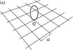
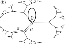
Figure 4: A diffusive ring attached to (a) : an infinite square lattice, (b) : an infinite Bethe lattice of coordinence $z=3$. In both cases the bonds have equal lengths $a$.

First we consider the network without the loop. It is characterized by a matrix whose determinant gives the spectral determinant $S_{\rm net}(\gamma)$.

If we now attach a ring at the vertex $\mathrm{𝟎}$ of the network, the new network is characterized by a matrix ${\cal M}={\cal M}_{\rm net}+\delta{\cal M}$ with

$$\delta{\cal M}_{\alpha\beta}=A(\theta,\lambda_{0})\,\delta_{\alpha 0}\delta_{\beta 0}$$ (33)

where (appendix C of [7])

$$A(\theta,\lambda_{0})=\lambda_{0}+2\sqrt{\gamma}\,\frac{\cosh\sqrt{\gamma}L-\cos\theta}{\sinh\sqrt{\gamma}L}\>.$$ (34)

Since $\delta{\cal M}$ has only one nonzero element, $(\delta{\cal M})_{00}$, we have

$$\det{\cal M}=\left[1+A(\theta,\lambda_{0})\,({\cal M}_{\rm net}^{-1})_{00}\right]\>\det{\cal M}_{\rm net}\>.$$ (35)

This shows that the spectral determinant of the network with the loop is now

$$S^{(\lambda_{0})}(\gamma)=\frac{\sinh\sqrt{\gamma}L}{\sqrt{\gamma}}\left[1+A(\theta,\lambda_{0})\,({\cal M}_{\rm net}^{-1})_{00}\right]\>S_{\rm net}(\gamma)\>.$$ (36)

Using (11) we have $P_{c}(0,0)=\frac{{\rm d}}{{\rm d}\lambda_{0}}\ln[1+A(\theta,\lambda_{0})\,({\cal M}_{\rm net}^{-1})_{00}]\big{|}_{\lambda_{0}=0}$ that leads to the same result (27,28) as when the ring is connected to an arm. It is interesting to note that the matrix element is related to the Green’s function of the diffusion operator in the network, i.e. the cooperon at the vertex $\mathrm{𝟎}$ in the absence of the ring :

$$P_{c}^{\rm net}(0,0)=\langle\kern 1.29167pt0\kern 1.29167pt|\frac{1}{\gamma-\Delta}|\kern 1.29167pt0\kern 1.29167pt\rangle=({\cal M}_{\rm net}^{-1})_{00}\>.$$ (37)

Therefore we can write the cooperon at the vertex $\mathrm{𝟎}$ in terms of the cooperon of the network in the absence of the ring :

$$P_{c}(0,0)=\frac{1}{2\sqrt{\gamma}}\frac{\sinh\sqrt{\gamma}L}{\cosh\sqrt{\gamma}L+\frac{1}{2}\frac{\sinh\sqrt{\gamma}L}{\sqrt{\gamma}P_{c}^{\rm net}(0,0)}-\cos\theta}\>.$$ (38)

Now the effective perimeter is related to the matrix ${\cal M}_{\rm net}$ characterizing the network in the absence of the loop :

$$\cosh\sqrt{\gamma}L_{\rm eff}=\cosh\sqrt{\gamma}L+\frac{1}{2}\frac{\sinh\sqrt{\gamma}L}{\sqrt{\gamma}\,({\cal M}_{\rm net}^{-1})_{00}}\>,$$ (39)

which is a generalization of the results (15,17) obtained for the ring attached to an arm. We can easily check that if the network is simply a wire with Dirichlet boundary at one end, we have $({\cal M}_{\rm net}^{-1})_{00}=1/(\sqrt{\gamma}\coth\sqrt{\gamma}b)$, leading to (15). In the limit $\sqrt{\gamma}L\ll 1$ (i.e. $L\ll L_{\varphi}$), eq. (39) leads to

$$\sqrt{\gamma}L_{\rm eff}\simeq\sqrt{\frac{L}{({\cal M}_{\rm net}^{-1})_{00}}}=\sqrt{\frac{L}{P_{c}^{\rm net}(0,0)}}\>.$$ (40)

The case of regular networks.– It is interesting to consider the specific case of a regular network. In this case we can write : ${\cal M}_{\rm net}=\frac{\sqrt{\gamma}}{\sinh\sqrt{\gamma}a}N$ where the matrix $N$ is $N_{\alpha\beta}=\delta_{\alpha\beta}\,z\cosh\sqrt{\gamma}a-a_{\alpha\beta}$. The matrix $a_{\alpha\beta}$ is the connectivity matrix (see appendix A). We have introduced the coordinence $z$ of the network. In this case ${\cal M}_{\rm net}^{-1}$ is related to the (discrete) Green’s function of the connectivity matrix $G(\alpha,\beta)=(N^{-1})_{\alpha\beta}$, defined by $\sum_{\mu}(E\,\delta_{\alpha\mu}-a_{\alpha\mu})G(\mu,\beta)=\delta_{\alpha\beta}$, for an “energy” $E=z\cosh\sqrt{\gamma}a$. It follows that the effective length is related to the discrete Green’s function of the network at the point where the ring is attached

$$\cosh\sqrt{\gamma}L_{\rm eff}=\cosh\sqrt{\gamma}L+\frac{1}{2}\frac{\sinh\sqrt{\gamma}L}{\sinh\sqrt{\gamma}a\>G(0,0)}\>.$$ (41)

In the limit $\sqrt{\gamma}L\ll 1$, we have

$$\sqrt{\gamma}L_{\rm eff}\simeq\sqrt{\frac{\sqrt{\gamma}L}{\sinh(\sqrt{\gamma}a)\>G(0,0)}}\>.$$ (42)

5.1 Ring connected to a square network

We now apply these results to the case of a square lattice. The problem left is to estimate the discrete Green’s function of the square network (figure 4a). We have

$$G(0,0)=\frac{1}{2}\int_{-\pi}^{+\pi}\frac{{\rm d}^{2}\vec{k}}{(2\pi)^{2}}\frac{1}{2\cosh\sqrt{\gamma}a-\cos k_{x}-\cos k_{y}}=\frac{1}{2\pi\cosh\sqrt{\gamma}a}\>{\rm K}\!\left(\frac{1}{\cosh\sqrt{\gamma}a}\right)$$ (43)

where ${\rm K}(x)$ is the complete elliptic integral of first kind. We have a new characteristic time $\tau_{a}=a^{2}$ needed to explore the bond. We now consider two limits of interest:

$\bullet$ Intermediate time $\tau_{L}\ll t\ll\tau_{a}$ (i.e. $L\ll L_{\varphi}\ll a$).– In this limit the Brownian trajectories starting from the ring can only explore a small portion of the 4 arms to which it is connected. Eq. (43) gives $L_{\rm eff}\simeq\sqrt{4L}\gamma^{-1/4}$. This result corresponds precisely to the case of a ring connected to $N_{a}=4$ long arms and we have $\int_{0}^{\infty}{\rm d}t\,W_{n}(0,0;t)\,{\mbox{\large e}}^{-\gamma t}\propto\exp-n\sqrt{4L}\gamma^{1/4}$.

$\bullet$ Long time $\tau_{L},\tau_{a}\ll t$ (i.e. $L,a\ll L_{\varphi}$).– In this case the Brownian trajectories encircling the flux $n$ times can explore the square network over distances much larger than $a$. Eq. (43) leads to

$$\sqrt{\gamma}\,L_{\rm eff}\simeq\sqrt{\frac{2\pi L}{a\ln(4/\sqrt{\gamma}a)}}\>.$$ (44)

The probability then reads

$$\int_{0}^{\infty}{\rm d}t\,W_{n}(0,0;t)\,{\mbox{\large e}}^{-\gamma t}\simeq\sqrt{\frac{La}{8\pi}\ln(4/\sqrt{\gamma}a)}\>\exp-n\sqrt{\frac{2\pi L}{a\ln(4/\sqrt{\gamma}a)}}\>.$$ (45)

The Brownian trajectories encircling the ring can leak over long distances in the square network. The effective diffusion in the ring is even slowed down compare to the case of a ring connected to arms. The number of windings behaves like :

$$n_{t}\simeq\sqrt{\frac{a}{\pi L}\ln t}\>$$ (46)

(the way to obtain the precise coefficient is explained in the appendix B). An argument similar to the one of section 4.2 can be developed to obtain (46) by different means. Since the diffusion is recurrent in the square network, this latter acts as a trap in which the diffusive particle stays during a time $\tau$ and eventually come back inside the ring. The distribution of the trapping time is given by the first return probability in a square lattice, that is known to behave at large times like $P_{1}(\tau)\propto 1/(\tau\ln^{2}\tau)$ [12] . It can be shown from this distribution that the winding number scales like $n_{t}\propto\sqrt{\ln t}$ [13].

The result (45) can be interpreted as the amplitude of the $n$-th harmonic of the AAS oscillations of the conductivity :

$$\Delta\sigma^{(n)}\propto\exp-n\sqrt{\frac{2\pi L}{a\ln(4L_{\varphi}/a)}}\hskip 14.22636pt\mbox{for }L,a\ll L_{\varphi}\>.$$ (47)

5.2 Ring connected to networks of higher dimensions

To emphasize the role of the dimension of the network, let us consider a $d$-dimensional hypercubic network. The Green’s function reads $G(0,0)=\frac{1}{2}\int_{\rm BZ}\frac{{\rm d}^{d}\vec{k}}{(2\pi)^{d}}\,[d\cosh\sqrt{\gamma}a-\sum_{i=1}^{d}\cos k_{i}]^{-1}$, where the integration is performed over the Brillouin zone. This can be conveniently rewritten $G(0,0)=\frac{1}{2}\int_{0}^{\infty}{\rm d}y\,[{\mbox{\large e}}^{-y\cosh\sqrt{\gamma}a}I_{0}(y)]^{d}$ where $I_{0}(y)$ is the modified Bessel function. (i) In dimension $d=1$ and $d=2$, the integral is dominated by the neighbourhood of $\vec{k}\sim 0$ (or the domain of large $y$) in the limit $\sqrt{\gamma}a\ll 1$. We can write $G(0,0)\simeq\int_{\rm BZ}\frac{{\rm d}^{d}\vec{k}}{(2\pi)^{d}}\,\frac{1}{\vec{k}^{2}+\gamma a^{2}d/2}$ or $G(0,0)\simeq\frac{1}{2}\int^{\infty}{\rm d}y\,\frac{1}{(2\pi y)^{d/2}}{\mbox{\large e}}^{-y\gamma a^{2}d/2}$. In dimension $d=1$ the integral diverges as $G(0,0)\sim 1/a\sqrt{\gamma}$, which reflects the recurrence of the 1d Brownian motion and leads to $\sqrt{\gamma}L_{\rm eff}\sim\gamma^{1/4}L^{1/2}$. The dimension $d=2$ is the marginal case : the integral diverges logarithmically $G(0,0)\sim\ln(1/a\sqrt{\gamma})$ which still indicates a recurrent Brownian motion and gives (44). (ii) In dimension $d>2$ the integral reaches a finite value $G(0,0)=\frac{1}{2}\int_{0}^{\infty}{\rm d}y\,[{\mbox{\large e}}^{-y}I_{0}(y)]^{d}=\beta_{d}$ in the limit $\gamma\to 0$. Note that $\beta_{d}\simeq 1/(2d)$ for large dimensions, that coincides with the result given below for a Bethe lattice of coordinence $z=2d$. The Brownian motion is not recurrent. Therefore $\sqrt{\gamma}L_{\rm eff}$ is independent on $\gamma$, which indicates that the winding number $n_{t}$ reaches a finite value in the infinite time limit.

Bethe lattice.– Let us consider the case of the Bethe lattice of coordinence $z$ (figure 4b), that models a network with an infinite effective dimension. The Green’s function at coinciding point is [14]

$$G(0,0)=\frac{1}{E}F_{0}\left(\frac{z}{E}\right)\hskip 7.11317pt\mbox{ with }\hskip 7.11317ptF_{0}(x)=\frac{2(z-1)}{z-2+\sqrt{z^{2}-4(z-1)x^{2}}}\>.$$ (48)

We obtain the following behaviour for $t\gg\tau_{L},\,\tau_{a}$

$$\int_{0}^{\infty}{\rm d}t\,W_{n}(0,0;t)\,{\mbox{\large e}}^{-\gamma t}\propto\exp-n\sqrt{\frac{z(z-2)}{z-1}\frac{L}{a}}\>.$$ (49)

This result is similar to the one obtained for a ring connected to an arm with absorption at the end (Dirichlet condition). In this latter case the absorption at the end of the arm is responsible from the fact that the particle leaves the ring after a finite time. In the Bethe lattice, since the diffusion is not recurrent, the diffusive particle injected in the ring eventually get lost in the infinite lattice. At large times the number of windings in the ring reaches the finite limit :

$$n_{t}\simeq\sqrt{\frac{2(z-1)}{z(z-2)}\frac{a}{L}}\>.$$ (50)

The higher the coordinence, the smaller the time spent by the particle in the ring is. The shorter $a$, the faster the particle feels the structure of the Bethe lattice and get lost in it.

All results are summarized in table 1.

Network	Regime	$L_{\rm eff}(\gamma)$	winding	$n^{2}_{t}$
no	$t\ll\tau_{L}$	$L$	normal	$2\exp-\frac{L^{2}}{4t}$
	$\tau_{L}\ll t$	$L$	normal	$2t/L^{2}$
$N_{a}$ arms	$t\ll\tau_{L},\,\tau_{b}$	$L$	normal	$2\exp-\frac{L^{2}}{4t}$
	$\tau_{L}\ll t\ll\tau_{b}$	$\sqrt{N_{a}LL_{\varphi}}$	anomalous	$2\sqrt{\pi t}/(N_{a}L)$
Neumann		$\sqrt{L(L+N_{a}b)}$	normal	$2t/(L^{2}+N_{a}bL)$
Dirichlet	$\tau_{L},\,\tau_{b}\ll t$	$L_{\varphi}\sqrt{N_{a}L/b}$	limited	$2b/(N_{a}L)$
square	$\tau_{L}\ll t\ll\tau_{a}$	$\sqrt{4LL_{\varphi}}$	anomalous	$\sqrt{\pi t}/(2L)$
	$\tau_{L},\,\tau_{a}\ll t$	$L_{\varphi}\sqrt{\frac{2\pi L}{\ln(4L_{\varphi}/a)}}$	anomalous	$\frac{a}{\pi L}\ln(t)$
$d$-hypercubic	$\tau_{L}\ll t\ll\tau_{a}$	$\sqrt{2dLL_{\varphi}}$	anomalous	$\sqrt{\pi t}/(dL)$
$d>2$	$\tau_{L},\,\tau_{a}\ll t$	$L_{\varphi}\sqrt{\frac{1}{\beta_{d}}\frac{L}{a}}$	limited	$2\beta_{d}\frac{a}{L}$
Bethe	$\tau_{L}\ll t\ll\tau_{a}$	$\sqrt{zLL_{\varphi}}$	anomalous	$2\sqrt{\pi t}/(zL)$
	$\tau_{L},\,\tau_{a}\ll t$	$L_{\varphi}\sqrt{\frac{z(z-2)}{z-1}\frac{L}{a}}$	limited	$\frac{2(z-1)}{z(z-2)}\frac{a}{L}$

Table 1: We summarize the results for the winding around the ring of perimeter $L$ connected to a network. We recall that $\gamma=1/L_{\varphi}^{2}$ allows to probe the various time regimes since it is the parameter conjugate to time : $\gamma\sim 1/t$. There are in general three characteristic times : the time $\tau_{L}=L^{2}$ to diffuse around the ring, the time $\tau_{a}=a^{2}$ to explore one bond of the network and the time $\tau_{b}=b^{2}$ to reach the boundary of the network of linear size $b$. Except for the case of the wire, we have considered infinite networks with $b=\infty$.

6 Conclusion

We have studied the winding properties inside a ring connected to a network. Our analysis was based on the introduction of the effective perimeter $L_{\rm eff}(\gamma)$ that probes the winding at time scale $t\sim 1/\gamma$. We have obtained this effective perimeter as a function of the matrix ${\cal M}_{\rm net}$ describing the network that is connected to the ring. The analysis of the effective perimeter immediatly gives the nature of the winding (normal or anomalous) since the winding number scales with time as $n_{t}\sim\sqrt{t}/L_{\rm eff}(1/t)$.

Our study of winding properties was motivated by the physics of quantum transport through a ring. We have emphasized the importance of taking properly into account the external wires connecting the ring when studying quantum transport. Experimentally, the measurement of ratio of harmonics provides a direct way to extract the phase coherence length and its temperature dependence (this has been used very recently on large square networks [15]). In particular assuming an exponential behaviour $\exp-nL/L_{\varphi}$, given by (2), or the nonexponential $\exp-n\sqrt{2L/L_{\varphi}}$, given by (6), leads to very different temperature dependences of $L_{\varphi}(T)$. The figure 5 summarizes our main result : we have plotted the effective length as a function of $L_{\varphi}$. The linear behaviour at small $L_{\varphi}$, corresponds to (5) and the square root behaviour at large $L_{\varphi}$, to (6). Since the crossover between the two regimes occurs on the range $L\sim L_{\varphi}$, it is useful to know the nature of this crossover. We note that the effective perimeter for the ring with $N_{a}$ arms can be well approximated by $L_{\rm eff}\simeq\sqrt{L^{2}+N_{a}L_{\varphi}L}$ which interpolates between $L$ and $\sqrt{N_{a}L_{\varphi}L}$ (see inset of figure 5). Therefore the harmonics decay approximatively as $\exp-n\sqrt{(L/L_{\varphi})^{2}+N_{a}L/L_{\varphi}}$. It is clear from this approximation that the crossover, that occurs for $L_{\varphi}\simeq L/N_{a}$, can be more easily reached for a large number of arms. In a metallic ring, the phase coherence can reach several microns. Therefore, the regime $L_{\varphi}>L/N_{a}$ seems to be attainable experimentally.

Figure 5: The effective perimeter $L_{\rm eff}$ for the ring of figure 2 with $N_{a}=2$ arms, as a function of the phase coherence length. $L_{\rm eff}$ is given by eq. (24). We have taken the limit $b\gg L_{\varphi}$. The dashed line is the expansion for large phase coherence length $L_{\rm eff}=\sqrt{2L_{\varphi}L}(1+\frac{11}{48}\frac{L}{L_{\varphi}}+\cdots)$. The thin line is the linear expansion $L_{\rm eff}=L+L_{\varphi}\ln(9/4)+\cdots$ at small $L_{\varphi}$. In the inset, we compare the exact result with the approximation $\sqrt{L^{2}+2L_{\varphi}L}$ (dotted line).

The phase coherence length $L_{\varphi}$ has been introduced as an effective parameter $\gamma=1/L_{\varphi}^{2}$ in the cooperon $P_{c}(x,x^{\prime})=\langle\kern 1.29167ptx\kern 1.29167pt|\frac{1}{\gamma-\Delta}|\kern 1.29167ptx^{\prime}\kern 1.29167pt\rangle$ in order to describe phase breaking mechanisms. However, the effect of electron-electron interactions, that dominates at low temperature, is not well described by such an effective parameter [16]. It has been shown recently that the behaviour of the AAS harmonics in a ring behaves in this case as $\exp-nT^{1/2}L^{3/2}$ in the limit $L_{\varphi}\ll L$ , where $T$ is the temperature [17]. However this behaviour has not been observed in the recent experiments [15] on large square networks, in which the condition $L_{\varphi}\ll L$ is not well fulfilled. A mechanism similar to the one discussed in our paper could explain the discrepancy between the theory and the experiment : for $L_{\varphi}\gtrsim L$ the excursion of the Brownian curves of finite winding in the surrounding part of the network increases the effective perimeter of these paths and modifies the dependence of the harmonics in $L/L_{\varphi}$.

Appendix A Spectral determinant

A particularly convenient way to describe the spectrum $\{E_{n}\}$ of the Laplace operator $\Delta$ on a network of one-dimensional wires is to consider the spectral determinant $S(\gamma)=\det(\gamma-\Delta)=\prod_{n}(\gamma+E_{n})$ where $\gamma$ is the spectral parameter. If the loops of the network are pierced by magnetic fluxes the derivative is replaced by the covariant derivative : $\Delta\to{\rm D}_{x}^{2}$ with ${\rm D}_{x}=\frac{{\rm d}}{{\rm d}x}-{\rm i}A(x)$.

Let us consider a network of $B$ wires connected at $V$ vertices. These latters are labelled with greek indices $\alpha$, $\beta$,…First we introduce the connectivity matrix $a_{\alpha\beta}$ characterizing the topology of the network : $a_{\alpha\beta}=1$ is $\alpha$ are $\beta$ connected by a bond (we denote $(\alpha\beta)$ the bond and $l_{\alpha\beta}$ its length). $a_{\alpha\beta}=0$ otherwise. If we define a scalar function $\psi(x)$ on the network, boundary conditions at the vertices must be specified. At the vertex $\alpha$ we choose (i) continuity of the function, that is all the components $\psi_{\alpha\beta}(x)$ of the function along the wires $\alpha\beta$ issuing from $\alpha$ tend to the same limit as the coordinate reaches the vertex. (ii) $\sum_{\beta}a_{\alpha\beta}{\rm D}_{x}\psi_{\alpha\beta}(\alpha)=\lambda_{\alpha}\psi(\alpha)$ where the connectivity matrix in the sum constrains it to run over the neighbouring vertices of $\alpha$. Therefore the sum runs over all wires issuing from the vertex. The real parameter $\lambda_{\alpha}$ allows to describe several boundary condition: $\lambda_{\alpha}=\infty$ forces the function to vanish, $\psi(\alpha)=0$, and corresponds to Dirichlet boundary condition that describes the connection to a reservoir that absorbs particles. $\lambda_{\alpha}=0$ corresponds to Neumann condition, which ensures conservation of the probability current and describes an internal vertex.

It was shown in [6] that the spectral determinant is :

$$S(\gamma)=\prod_{(\alpha\beta)}\frac{\sinh\sqrt{\gamma}l_{\alpha\beta}}{\sqrt{\gamma}}\>\det{\cal M}(\gamma)$$ (51)

where the product runs over all bonds of the network. ${\cal M}$ is a $V\times V$ matrix defined as :

$${\cal M}_{\alpha\beta}=\delta_{\alpha\beta}\left(\lambda_{\alpha}+\sqrt{\gamma}\sum_{\mu}a_{\alpha\mu}\coth(\sqrt{\gamma}l_{\alpha\mu})\right)-a_{\alpha\beta}\frac{\sqrt{\gamma}\>{\mbox{\large e}}^{-{\rm i}\theta_{\alpha\beta}}}{\sinh(\sqrt{\gamma}l_{\alpha\beta})}\>,$$ (52)

where the connectivity matrix constrains the sum to run over all vertices $\mu$ connected to $\alpha$. We have included the magnetic fluxes ($\theta_{\alpha\beta}$ is the flux along the wire). For a more detailed presentation, see [7].

Appendix B Time dependence of the winding number

We explain how to compute efficiently the time dependence of the winding number around a ring connected to a network. For this purpose we compute $\langle n^{2}\rangle_{t}$, where the average is taken for all close trajectories starting from a specified point and coming back to it after a time $t$ :

$$\langle n^{2}\rangle_{t}=\frac{\sum_{n}n^{2}\,W_{n}(x,x;t)}{\sum_{n}W_{n}(x,x;t)}\>$$ (53)

($\langle n\rangle_{t}=0$ follows from the symmetry $P_{c}|_{\theta}=P_{c}|_{-\theta}$).

To go further we consider the case where the initial condition $x$ is the vertex $\mathrm{𝟎}$ where the ring is attached to the network. Then the cooperon has the structure (27). Let us define the quantity

$$\Omega_{m}(\gamma)=\left(\frac{1}{{\rm i}}\frac{{\rm d}}{{\rm d}\theta}\right)^{m}P_{c}(0,0)\big{|}_{\theta=0}\>.$$ (54)

From (9) it follows that $\Omega_{m}(\gamma)=\int_{0}^{\infty}{\rm d}t\,{\mbox{\large e}}^{-\gamma t}\sum_{n}n^{m}W_{n}(0,0;t)$ which is related to the $m$-th moment of the winding number. We have

$$\langle n^{2}\rangle_{t}=\frac{{\cal L}^{-1}\left[\Omega_{2}(\gamma)\right]}{{\cal L}^{-1}\left[\Omega_{0}(\gamma)\right]}$$ (55)

where ${\cal L}^{-1}\left[\cdots\right]$ designates the inverse Laplace transform. From (27) we can obtain the two general expressions :

$$\Omega_{0}(\gamma) = \frac{1}{4\sqrt{\gamma}}\,\frac{\sinh\sqrt{\gamma}L}{\left(\sinh\frac{\sqrt{\gamma}L_{\rm eff}}{2}\right)^{2}}$$ (56)

$$\Omega_{2}(\gamma) = \frac{1}{8\sqrt{\gamma}}\,\frac{\sinh\sqrt{\gamma}L}{\left(\sinh\frac{\sqrt{\gamma}L_{\rm eff}}{2}\right)^{4}}\>.$$ (57)

Example 1 : the isolated ring.– The effective perimeter is equal to the perimeter in this case : $L_{\rm eff}=L$. We have $\Omega_{0}(\gamma)=\frac{1}{2\sqrt{\gamma}}\coth(\sqrt{\gamma}L/2)$ and $\Omega_{2}(\gamma)=\frac{1}{4\sqrt{\gamma}}\coth(\sqrt{\gamma}L/2)/\sinh^{2}(\sqrt{\gamma}L/2)$. We consider two regimes :
$\bullet$ Short times $t\ll\tau_{L}$ : We have $\Omega_{0}(\gamma)\simeq\frac{1}{2\sqrt{\gamma}}$ and $\Omega_{2}(\gamma)\simeq\frac{1}{\sqrt{\gamma}}{\mbox{\large e}}^{-\sqrt{\gamma}L}$ which gives after Laplace transform $\langle n^{2}\rangle_{t}\simeq 2\exp-\frac{L^{2}}{4t}$. This result was obvious from the expression (13).
$\bullet$ Long times $t\gg\tau_{L}$ : We obtain in this case $\Omega_{0}(\gamma)\simeq\frac{1}{\gamma L}$ and $\Omega_{2}(\gamma)\simeq\frac{2}{\gamma^{2}L^{3}}$, which leads to $\langle n^{2}\rangle_{t}\simeq 2t/L^{2}$. This is the normal diffusion.

Example 2 : the ring connected to a square network.– We consider the long time limit $t\gg\tau_{L},\tau_{a}$ to demonstrate (46). The effective perimeter is given by (44). We find $\Omega_{0}(\gamma)\simeq\frac{a}{4\pi}\ln(16/a^{2}\gamma)$ and $\Omega_{2}(\gamma)\simeq\frac{a^{2}}{8\pi^{2}L}\ln^{2}(16/a^{2}\gamma)$. Using the fact that in the limit $\gamma\to 0$ we have ${\cal L}^{-1}\left[\ln 1/\gamma\right]\simeq 1/t$ and ${\cal L}^{-1}\left[\ln^{2}1/\gamma\right]\simeq 2\ln(t)/t$, we eventually find $\langle n^{2}\rangle_{t}\simeq\frac{a}{\pi L}\ln t$.

References

- [1] B. L. Al’tshuler, A. G. Aronov, and B. Z. Spivak, The Aaronov-Bohm Effect in disordered conductors, JETP Lett. 33(2), 94 (1981).
- [2] C. Texier and G. Montambaux, Weak localization in multiterminal networks of diffusive wires, Phys. Rev. Lett. 92, 186801 (2004).
- [3] C. Texier, G. Montambaux, and E. Akkermans, to be published (2005).
- [4] A. Comtet, J. Desbois, and S. Ouvry, Winding of planar Brownian curves, J. Phys. A: Math. Gen. 23, 3563 (1990).
- [5] C. Monthus, Étude de quelques fonctionnelles du mouvement brownien et de certaines propriétés de la diffusion unidimensionnelle en milieu aléatoire, PhD thesis, Université Paris 6, 1995.
- [6] M. Pascaud and G. Montambaux, Persistent currents on networks, Phys. Rev. Lett. 82, 4512 (1999).
- [7] E. Akkermans, A. Comtet, J. Desbois, G. Montambaux, and C. Texier, On the spectral determinant of quantum graphs, Ann. Phys. (N.Y.) 284, 10 (2000).
- [8] G. H. Weiss and S. Havlin, Some properties of a random walk on a comb structure, Physica 134A, 474 (1986).
- [9] R. C. Ball, S. Havlin, and G. H. Weiss, Non-Gaussian random walks, J. Phys. A: Math. Gen. 20, 4055 (1987).
- [10] J.-P. Bouchaud and A. Georges, Anomalous diffusion in disordered media: Statistical mechanisms, models and physical applications, Phys. Rep. 195, 267 (1990).
- [11] É. Akkermans and G. Montambaux, Physique mésoscopique des électrons et des photons, EDP Sciences, CNRS éditions, 2004.
- [12] A. V. Barzykin and M. Tachiya, Diffusion-influenced reaction kinetics on fractal structures, J. Chem. Phys. 99, 9591 (1993).
- [13] S. N. Majumdar, private communication (2004).
- [14] C. Monthus and C. Texier, Random walk on the Bethe lattice and hyperbolic Brownian motion, J. Phys. A: Math. Gen. 29, 2399 (1996).
- [15] M. Ferrier, L. Angers, A. C. H. Rowe, S. Guéron, H. Bouchiat, C. Texier, G. Montambaux, and D. Mailly, Direct measurement of the phase coherence length in a GaAs/GaAlAs square network, preprint cond-mat/0402534 (2004), to appear in Phys. Rev. Lett.
- [16] B. L. Altshuler, A. G. Aronov, and D. E. Khmelnitsky, Effects of electron-electron collisions with small energy transfers on quantum localisation, J. Phys. C: Solid St. Phys. 15, 7367 (1982).
- [17] T. Ludwig and A. D. Mirlin, Interaction-induced dephasing of Aharonov-Bohm oscillations, Phys. Rev. B 69, 193306 (2004).