Nonperturbative Effects on $T_{c}$ of Interacting Bose Gases in Power-Law Traps

Abstract

The critical temperature $T_{c}$ of an interacting Bose gas trapped in a general power-law potential $V({\bf x})=\sum_{i}U_{i}|x_{i}|^{p_{i}}$ is calculated with the help of variational perturbation theory. It is shown that the interaction-induced shift in $T_{c}$ fulfills the relation $(T_{c}-T_{c}^{0})/T_{c}^{0}=D_{1}(\eta)\hat{a}+D^{\prime}(\eta)\hat{a}^{2\eta}+{\cal O}(\hat{a}^{2})$ with $T_{c}^{0}$ the critical temperature of the trapped ideal gas, $\hat{a}$ the $s$-wave scattering length divided by the thermal wavelength at $T_{c}$, and $\eta=1/2+\sum_{i}p_{i}^{-1}$ the potential-shape parameter. The terms $D_{1}(\eta)\hat{a}$ and $D^{\prime}(\eta)\hat{a}^{2\eta}$ describe the leading-order perturbative and nonperturbative contributions to the critical temperature, respectively. This result quantitatively shows how an increasingly inhomogeneous potential suppresses the influence of critical fluctuations. The appearance of the $\hat{a}^{2\eta}$ contribution is qualitatively explained in terms of the Ginzburg criterion.

I Introduction

The realization of Bose-Einstein condensation (BEC) in dilute atomic vapors has renewed interest in the critical properties of weakly interacting Bose gases and, in particular, their transition temperature $T_{c}$. Important recent work in this area concerns the role of the external trapping potential. For the homogeneous Bose gas, the shift in $T_{c}$ caused by $s$-wave contact interactions is in leading order completely due to long-wavelength, critical fluctuations that have to be described nonperturbatively. It is now established that these fluctuations lead to a linear increase of the critical temperature with the $s$-wave scattering length $a$, if the particle density is fixed BayBlaHol99 ; ArnMooTom01 ; ArnMoo01 ; KasProSvi01 . A harmonic trapping potential, on the other hand, suppresses the critical long-wavelength fluctuations and reduces the fraction of atoms taking part in nonperturbative physics at the transition point. As a result, the leading-order shift in $T_{c}$ can be calculated by simple pertubative methods, for instance the mean-field (MF) approximation to the Landau-Pitaevskii equation GioPitStr96 ; ArnTom01 . Interestingly, the shift here is a decreasing linear function of the scattering length $a$.

Work on the critical temperature of Bose gases has so far been mainly concerned with homogeneous and harmonically trapped systems. As outlined above, in these two situations very different physical mechanisms determine the shift of $T_{c}$. This observation naturally motivates an investigation of the crossover between the two cases. In this paper we shall interpolate between these limits by studying the condensation in a general power-law potential, whose parameters can be varied continuously. In this way we shall obtain a deeper understanding of how the increasing inhomogeneity of the potential suppresses the critical fluctuations and changes nonperturbative into perturbative physics. The power-law potentials under study are given by

$$V({\bf x})=\sum_{i=1}^{3}E_{i}\left|\frac{x_{i}}{L_{i}}\right|^{p_{i}}$$ (1)

with $E_{i}$ and $L_{i}$ denoting energy and length scales. If all powers $p_{i}$ are set equal to $2$, we recover the harmonic potential, whereas in the limit of all $p_{i}$ diverging, $V({\bf x})$ approaches a box shape characteristic of the homogeneous Bose gas.

First investigations of the crossover behavior of the critical temperature in these potentials were recently reported in Refs. Zob04 ; ZobMetAlb04 . In Zob04 , the shift in $T_{c}$ for these potentials was determined within mean-field theory in the thermodynamic limit. Extending earlier first-order calculations ShiZhe97a ; PI , it was shown that up to second order in the scattering length $a$, the MF shift has an expansion

$$\frac{T_{c}-T_{c}^{0}}{T_{c}^{0}}=D_{1}^{(MF)}(\eta)\hat{a}+D^{\prime}_{(MF)}(\eta)\hat{a}^{2\eta}+D_{2}^{(MF)}(\eta)\hat{a}^{2}+o(\hat{a}^{2})$$ (2)

with $T_{c}^{0}$ the critical temperature of the noninteracting gas, and $\hat{a}\equiv a/\lambda_{T_{c}}$ the scattering length measured in units of the thermal wavelength $\lambda_{T}\equiv\sqrt{2\pi\hbar^{2}/k_{B}Tm}$ for particles of mass $m$ at a temperature $T$. The exponent of the second term is twice the shape parameter of the potential,

$$\eta=\sum_{i=1}^{3}\frac{1}{p_{i}}+\frac{1}{2},$$ (3)

so that $2\eta$ grows from $1$ to $4$ as the shape changes from homogeneous to harmonic. The coefficients $D^{\prime}_{(MF)}(\eta)$ and $D_{1,2}^{(MF)}(\eta)$ are respectively given explicitly or through simple quadratures. These results provided first insights into the crossover in the behavior of $T_{c}$ between homogeneous and inhomogeneous potentials. However, since mean-field theory does not account for critical fluctuations, it can only provide a rough first estimate, especially in the quasi-homogeneous regime, and needs to be improved by more sophisticated methods.

One possible pathway for taking critical fluctuations into account was explored in Ref. ZobMetAlb04 , where the shift in $T_{c}$ was calculated with the help of a renormalization group (RG) method initially developed for studying the harmonically trapped gas MetZobAlb04 . The results were found to be in good qualitative agreement with mean-field theory. As a main advantage, the RG approach employed in that work gave a simple and transparent tool to compute the critical temperature for a wide range of potential shapes and interaction strengths. A disadvantage was, however, that the results were mainly numerical and rendered only limited physical insight into the system. Furthermore, the calculation required several unsystematic approximations which are difficult to improve.

The purpose of this paper is to present a more systematic approach to the problem by making use of field-theoretic variational perturbation theory (VPT). VPT is a powerful resummation method for divergent perturbation series PI , which has been extended to quantum field theory and its anomalous dimensions in Ref. SCT ; KS . It has led to a prediction of the critical exponents of superfluid helium with unprecedented accuracy SCT2 ; KS , as confirmed for the exponent $\alpha$ of the specific heat of helium by satellite experiments Lipa .

In the context of BEC, field-theoretic VPT has been applied successfully to determine the shift of the critical temperature of the homogeneous Bose gas from a five-loop perturbation expansion Kle03 , extended recently to six and seven loops in Kas03 . In the present work we shall describe the trapped Bose gas in the thermodynamic limit, in which the trap is so wide that we may apply, as in Zob04 ; ZobMetAlb04 , the local-density approximation (LDA). The system is treated as locally homogeneous at any point ${\bf x}$ with an effective chemical potential $\mu_{\rm eff}=\mu-V({\bf x})$, where $\mu$ denotes the global chemical potential. In this way, we can make contact with the high-order perturbative loop expansions that were derived in Refs. Kle03 ; Kas03 for classical three-dimensional $\phi^{4}$-theories of homogeneous systems. Because of dimensional reduction Zin89 , the effective classical theory FK ; PI can be directly used to describe critical properties of the (quantum-mechanical) Bose gas below second order in the scattering length BayBlaHol99 ; ArnMooTom01 .

In this work we shall combine the high-order loop expansions with the LDA to derive a perturbative expansion for the particle number of the trapped system in powers of ${\hat{a}}=a/\lambda_{T}$. From this expansion we extract, with the help of field-theoretic VPT, the critical particle number and the shift of $T_{c}$. The main results are: (i) For small ${\hat{a}}$, the shift of $T_{c}$ is shown to exactly follow a behavior $(T_{c}-T_{c}^{0})/T_{c}^{0}=D_{1}(\eta)\hat{a}+D^{\prime}(\eta)\hat{a}^{2\eta}+{\cal O}({\hat{a}}^{2})$ in generalization of the mean-field result (2). The term proportional to ${\hat{a}}^{2\eta}$ represents the leading nonperturbative effects, whereas $D_{1}(\eta)$ can be calculated perturbatively as discussed in Zob04 ; ShiZhe97a . The second-order contribution, which we will not study in detail, contains terms proportional to $\hat{a}^{2}$ and $\hat{a}^{2}\ln\hat{a}$. (ii) We compute the coefficient $D^{\prime}(\eta)$ for $\eta<1$ using VPT, and in this way arrive at a quantitative description of the behavior of $T_{c}$ below second order in the scattering length. (iii) Following ArnTom01 , we give a qualitative explanation for the ${\hat{a}}^{2\eta}$ behavior of $T_{c}$ based on the Ginzburg criterion GI .

The paper is organized as follows. In Sec. II, the physics of ideal Bose gases in power-law potentials is briefly reviewed. In Sec. III we show with the help of general scaling arguments why the critical temperature obeys a law of the form (2), and give a physical interpretation for the appearance of the nonanalytic term. Section IV contains the calculation of the nonperturbative coefficient $D^{\prime}(\eta)$, and illustrates the behavior of the critical temperature by means of a numerical example. Summary and conclusions are given in Sec. V.

II Ideal Bose gases in power-law traps

In this section we summarize some known properties of ideal Bose gases in power-law traps that are needed later. The notation follows Refs. ShiZhe97a and BagPriKle87 . We consider a system of $N$ ideal bosons of mass $m$ trapped in the power-law potential (1) characterized by the shape parameter $\eta$ introduced in Eq. (3). We define the characteristic volume by

$$V_{{\rm char}}^{2(\eta+1)/3}=8\left(\frac{\hbar^{2}}{m}\right)^{\eta-\frac{1}{2}}\prod_{i=1}^{3}\frac{I(p_{i})L_{i}}{E_{i}^{{1}/{p_{i}}}},$$ (4)

where $I(p_{i})\equiv\Gamma(1/p_{i})/p_{i}$ and $\Gamma(z)$ denotes the usual gamma function. The quantity $V_{{\rm char}}$ provides an estimate for the volume occupied by the one-particle ground state in the trap.

For calculations in the local-density approximation it is useful to convert spatial integrations involving the trap potential into energy integrations according to the rule $\int d^{3}x\,f[V({\bf x})]=\int d\varepsilon\tilde{\rho}(\varepsilon)f(\varepsilon)$. In this way, we can easily deal with power-law potentials of any type. The density $\tilde{\rho}(\varepsilon)$ is the area of the equipotential surface $V({\bf x})=\varepsilon$. As shown in Zob04 ; ZobMetAlb04 , $\tilde{\rho}(\varepsilon)$ is given by

$$\tilde{\rho}(\varepsilon)=\frac{V_{{\rm char}}^{2(\eta+1)/3}}{\Gamma(\eta-1/2)}\left(\frac{m}{\hbar^{2}}\right)^{\eta-1/2}\varepsilon^{\eta-3/2}.$$ (5)

As announced above, we shall treat the thermodynamic limit, in which $N$ and $V_{{\rm char}}$ go to infinity at fixed $N/V_{{\rm char}}^{2(\eta+1)/3}$. The equation of state for the ideal Bose gas above the condensation point is then given by LiCheChe99 ; Yan00

$$N=\frac{1}{(2\pi)^{3/2}}\left(\frac{m}{\hbar^{2}\beta}\right)^{\eta+1}V_{{\rm char}}^{2(\eta+1)/3}\zeta_{\eta+1}(z),$$ (6)

where $\beta\equiv 1/k_{B}T$ denotes the inverse temperature, $\mu$ the chemical potential, and $z=\exp(\beta\mu)$ the fugacity. The Bose-Einstein functions $\zeta_{\lambda}(z)\equiv\sum_{k=1}^{\infty}z^{k}/k^{\lambda}$ are polylogarithmic functions ch7 . The spatial density distribution of the gas is determined by the relation

$$n({\bf x})=\lambda_{T}^{-3}\zeta_{3/2}\left(e^{\beta[\mu-V({\bf x})]}\right).$$ (7)

The condition for Bose-Einstein condensation $N=\int d^{3}x\,n({\bf x},\mu=0)$ can be obtained from Eq. (6) by setting $z=1$ or directly from Eq. (7) and reads BagPriKle87

$$N=\frac{1}{(2\pi)^{3/2}}\left(\frac{m}{\hbar^{2}\beta_{c}^{0}}\right)^{\eta+1}V_{{\rm char}}^{2(\eta+1)/3}\zeta(\eta+1),$$ (8)

where we have replaced $\zeta_{\nu}(1)$ by Riemann’s $\zeta$-function $\zeta(\nu)=\sum_{n=1}^{\infty}1/n^{\nu}$, and $\beta_{c}^{0}=1/k_{B}T_{c}^{0}$ denotes the inverse critical temperature of the ideal gas.

III General behavior of critical temperature

We now turn to the interacting Bose gas where we assume, as usual, that the interaction is effectively a delta-function potential which is completely characterized by the $s$-wave scattering length $a$. In the local-density approximation to the thermodynamic limit, the trapped particle number $N$ at given temperature $T$ and chemical potential $\mu$ can be calculated from the integral

$$N(T,\mu)=\int d^{3}x\,n_{\rm tr}({\bf x};\mu,T)\approx\int d^{3}x\,n_{\rm hom}(\mu-V({\bf x}),T),$$ (9)

where $n_{\rm tr}$ is the trapped particle density and $n_{\rm hom}$ the density of the homogeneous gas. As we briefly explain at the end of this section, we expect the LDA to be applicable if the condition $\lambda_{T_{c}}^{2}/a\ll V_{\rm char}^{1/3}$ is fulfilled, where $\lambda_{T_{c}}$ denotes the thermal wavelength at the condensation point and $V_{\rm char}$ is defined in Eq. (4). Obviously, for a fixed $\lambda_{T_{c}}$ this condition can always be met by making the trap wide enough (and increasing the particle number accordingly).

In the following, we want to apply Eq. (9) to explain why the critical temperature follows a behavior as indicated in Sec. I. A more detailed calculation will be presented in Sec. IV. Consider the perturbation expansion of the homogeneous density $n_{\rm hom}$ in powers of $\hat{a}=a/\lambda_{T}$

$$n_{\rm hom}(T,\Delta\mu)=n_{\rm hom}^{(0)}(T,\Delta\mu)+n_{\rm hom}^{(1)}(T,\Delta\mu)\hat{a}+n_{\rm hom}^{(2)}(T,\Delta\mu)\hat{a}^{2}+{\cal O}\left(\hat{a}^{3}\right),$$ (10)

where $\Delta\mu\equiv\mu_{c}-\mu$ is the negative distance of the chemical potential $\mu$ from its critical value $\mu_{c}$ at temperature $T$. Our definition of $\Delta\mu$ ensures that it is positive above the transition.

The omitted higher-order terms in the expansion (10) depend on the details of the particle interactions. Being interested in contributions below second order, we can disregard these details and work only with a contact interaction. Note that in Eq. (10) we have neglected logarithmic terms appearing at second and higher order in $\hat{a}$. These terms enter via the critical chemical potential $\mu_{c}$ which contains a contribution proportional to $\hat{a}^{2}\ln\hat{a}$ ArnTom01 . As the calculation of Sec. IV shows, the omitted logarithmic terms are not relevant for determining the shift in $T_{c}$ below second order.

From Eq. (10), we can convince ourselves that there must exist a perturbative second-order contribution to the critical particle number. This justifies the inclusion of a term proportional to $\hat{a}^{2}$ in the general expression for the shift in $T_{c}$, as mentioned at the end of Sec. I. Indeed, since the expansion (10) becomes arbitrarily accurate when we go sufficiently far away from the critical region, we can split the spatial integral in Eq. (9) into a part near the trap center and a remainder:

$$N(T,\mu_{c})=\int_{V({\bf x})\leq V_{0}}d^{3}x\,n_{\rm hom}(\mu_{c}-V({\bf x}),T)+\int_{V({\bf x})>V_{0}}d^{3}x\,n_{\rm hom}(\mu_{c}-V({\bf x}),T).$$ (11)

Here, $V_{0}$ denotes an energy above which the perturbative expansion of the density becomes accurate. Inserting the expansion (10) into the second integral, we see that $N(T,\mu_{c})$ contains a contribution which is of second order in the scattering length. Since the expansion for $n_{\rm hom}$ contains a term proportional to $\hat{a}^{2}\ln\hat{a}$ as mentioned above, there will also be such a contribution in the exact second-order result (compare to Ref. ArnTom01 for the harmonic case).

The expansion coefficients $n_{\rm hom}^{(0)}$ and $n_{\rm hom}^{(1)}$ in the perturbation series (10) remain finite in the critical limit $\Delta\mu\to 0$. From Eq. (9) we thus obtain well-defined perturbative contributions to the critical particle number in zeroth and first order in $\hat{a}$. The zeroth-order contribution is just the critical particle number of the ideal gas. However, all other coefficients $n_{\rm hom}^{(i)}$, $i\geq 2$, are infrared-divergent in the critical limit of $\Delta\mu\to 0$ where they behave like $1/\sqrt{\Delta\mu}^{i-1}$. Nevertheless, as shown in Refs. Kle03 ; Kas03 , we can make use of resummation techniques to extract information about critical properties from the expansion. If we focus on effects below second order in the scattering length, it is sufficient to consider only the leading divergence $n_{\rm hom}^{(i,{\rm div})}$ at each order, i.e., $n_{\rm hom}^{(i)}=n_{\rm hom}^{(i,{\rm div})}+o((\Delta\mu)^{(i-1)/2})$. This leads to the power series

$$\Delta n_{\rm hom}^{\rm div}(T,\Delta\mu)\equiv\sum_{i=2}^{\infty}n_{\rm hom}^{(i,{\rm div})}(T,\Delta\mu)\hat{a}^{i}=\hat{a}\sum_{i=2}^{\infty}b_{i}\,\left(\frac{\hat{a}}{\sqrt{\beta\Delta\mu}}\right)^{i-1}.$$ (12)

Above the transition where the chemical potential $\mu$ is smaller than $\mu_{c}$ so that $\Delta\mu>0$, we insert (12) into (9) and obtain the leading-order divergent contribution to the trapped particle number

$$\Delta N^{{\rm div}}(T,\Delta\mu) = \!\!\!\int d^{3}x\,\Delta n_{\rm hom}^{{\rm div}}(T,\Delta\mu+V({\bf x}))=\!\hat{a}\int d^{3}x\,\sum_{i=2}^{\infty}b_{i}\left(\frac{\hat{a}}{\sqrt{\beta[\Delta\mu+V({\bf x})]}}\right)^{i-1}.$$ (13)

Converting the spatial integral into an energy integral with the help of (5) and performing this integral with analytic regularization, we obtain

$$\Delta N^{{\rm div}}(T,\Delta\mu) = \!\!\!A\int d\varepsilon\,\varepsilon^{\eta-3/2}\hat{a}\sum_{i=2}^{\infty}b_{i}\left(\frac{\hat{a}}{\sqrt{\beta(\Delta\mu+\varepsilon)}}\right)^{i-1}$$ (14)

$$= \!C(\Delta\mu)^{\eta}\sum_{i=2}^{\infty}b_{i}\left(\frac{\hat{a}}{\sqrt{\beta\Delta\mu}}\right)^{i}\frac{\Gamma(i/2-\eta)}{\Gamma(i/2-1/2)}$$

$$= (\Delta\mu)^{\eta}\,h_{1}\!\!\left(\frac{\hat{a}}{\sqrt{\beta\Delta\mu}}\right),$$

where irrelevant constants have been absorbed into the coefficients $A$ and $C$. Note that the factors $\Gamma(i/2-\eta)$ in the coefficients cause divergences for $\eta\to 1$. We ignore this issue for the moment and defer its discussion to Sec. IV. The main property of (14) is that the function $h_{1}$ in the final expression depends only on the ratio ${\hat{a}}/{\sqrt{\beta\Delta\mu}}$. If the number of particles is to remain finite in the critical limit $\Delta\mu\rightarrow 0$, the limiting behavior of $h_{1}({\hat{a}}/{\sqrt{\beta\Delta\mu}})$ must be $h_{1}({\hat{a}}/{\sqrt{\beta\Delta\mu}})\propto({\hat{a}}/{\sqrt{\beta\Delta\mu}})^{2\eta}$. It follows that the critical $\Delta N^{{\rm div}}$ behaves like $\hat{a}^{2\eta}$.

Combining this result with the perturbative first-order contribution mentioned above, we find that the change $\Delta N_{\rm crit}$ in the critical particle number at fixed temperature is given by

$$\frac{\Delta N_{\rm crit}}{N_{\rm crit}^{0}}=C_{1}(\eta)\hat{a}+C^{\prime}(\eta)\hat{a}^{2\eta}+{\cal O}(\hat{a}^{2})$$ (15)

with $N_{\rm crit}^{0}$ the critical particle number of the ideal gas, and $C_{1}(\eta)$, $C^{\prime}(\eta)$ proportionality constants depending on the potential shape. From this behavior we immediately deduce the change of the critical temperature at fixed particle number to behave like

$$\frac{\Delta T_{c}}{T_{c}^{0}}=D_{1}(\eta)\hat{a}+D^{\prime}(\eta)\hat{a}^{2\eta}+{\cal O}(\hat{a}^{2})$$ (16)

with coefficients $D_{1}(\eta)$ and $D^{\prime}(\eta)$ which follow trivially from $C_{1}(\eta)$ and $C^{\prime}(\eta)$ [compare with Eq. (25) below].

Figure 1: Schematic diagram of shift in $T_{c}$ for a fixed small scattering length $\hat{a}$ as a function of the potential shape parameter $\eta$. The upper curve shows the full result below second order according to Eq. (16), the dashed lower curve only displays the perturbative contribution linear in $\hat{a}$. The nonperturbative contribution decreases fast with growing inhomogeneity.

To discuss the physical contents of Eq. (16) we anticipate some of the results of the next section, and schematically show in Fig. 1 the behavior of the critical temperature at a fixed, small value of $\hat{a}$ as a function of the potential shape parameter $\eta$. The full curve shows the combined perturbative and nonperturbative contributions, whereas the dashed curve displays only the perturbative (linear) term. In the homogeneous limit we have $2\eta=1$, so that the shift below second order in $\hat{a}$ is purely linear as we expect from earlier studies BayBlaHol99 ; ArnMooTom01 ; HolBayBla01 . In this case, both contributions [i.e., $D_{1}(\eta)\hat{a}$ and $D^{\prime}(\eta)\hat{a}^{2\eta}$] are of comparable size at any value of $\hat{a}$.

The situation changes when we enter the inhomogeneous regime where $2\eta>1$. As displayed in Fig. 1, for sufficiently small, fixed $\hat{a}$ and growing $\eta$ the nonperturbative contribution $D^{\prime}(\eta)\hat{a}^{2\eta}$ rapidly becomes very small compared to the perturbative term. This kind of behavior is independent of the detailed form of $D^{\prime}(\eta)$ [note that in Fig. 1, we ignore the (unphysical) divergence of our approximation (16) in a narrow vicinity of $\eta=1$; as discussed in Sec. IV, this is expected to be remedied in a higher-order expansion]. Equation (16) describes quantitatively how the growing inhomogeneity of the potential reduces the influence of critical fluctuations on the transition temperature.

Following the arguments of Ref. ArnTom01 , we can also give a physical explanation for the appearance of the $\hat{a}^{2\eta}$ term by estimating the fraction of atoms actually taking part in nonperturbative effects. For simplicity, consider the potential $V({\bf x})=\sum_{i}V_{0}|x_{i}/r_{0}|^{\gamma}$. Treating the Bose gas above the transition point as classical, we find the mean-square width

$$\langle x_{i}^{2}\rangle=r_{0}^{2}\frac{\Gamma(3/\gamma)}{(\beta V_{0})^{2/\gamma}\Gamma(1/\gamma)},\quad i=1,2,3,$$ (17)

i.e., the cloud radius behaves like

$$r_{\rm cloud}\sim\frac{r_{0}}{(\beta V_{0})^{1/\gamma}}.$$ (18)

From the Ginzburg criterion GI it follows that nonperturbative effects only arise at (local) chemical potentials $\mu_{\rm eff}$, for which

$$\mu_{c}-\mu_{\rm eff}~{}\raise 1.29167pt\hbox{$<$\kern-7.5pt\raise-4.73611pt\hbox{$\sim$}}~{}\frac{\hbar^{2}a^{2}}{m\lambda_{T}^{4}}.$$ (19)

Invoking the local density approximation, this means that the nonperturbative region around the trap center has a radius of about

$$r_{\rm np}\sim r_{0}\left(\frac{\hbar^{2}a^{2}}{m\lambda_{T}^{4}V_{0}}\right)^{1/\gamma}.$$ (20)

The fraction of atoms within this nonperturbative spatial region is given by

$$\left(\frac{r_{\rm np}}{r_{\rm cloud}}\right)^{3}\sim\left(\frac{a}{\lambda_{T}}\right)^{6/\gamma}.$$ (21)

However, not all atoms within this region actually take part in nonperturbative physics ArnTom01 . From the homogeneous system we infer that only a fraction $a/\lambda_{T}$ are actually involved in these effects. For the trap, this means that the fraction of “nonperturbative” atoms scales like

$$\frac{a}{\lambda_{T}}\left(\frac{r_{\rm np}}{r_{\rm cloud}}\right)^{3}\sim\left(\frac{a}{\lambda_{T}}\right)^{(6/\gamma)+1}=\left(\frac{a}{\lambda_{T}}\right)^{2\eta},$$ (22)

which explains the appearance of the nonanalytic term in Eq. (15).

At this point, it is also convenient to explain the estimate for the validity of the LDA given above, again following the arguments of Ref. ArnTom01 . Nonperturbative effects involve fluctuations with wavelengths $\lambda_{T}^{2}/a$ and larger. For the LDA to be applicable, the size $r_{\rm np}$ of the nonperturbative region around the trap center should thus be much larger than $\lambda_{T}^{2}/a$. Since Eq. (20) can be rewritten as

$$r_{np}\sim\left(\frac{a}{\lambda_{T}}\right)^{2/\gamma}V_{\rm char}^{(2/\gamma+1)/3}$$

by using Eq. (4), this condition immediately implies that $\lambda_{T}^{2}/a\ll V_{\rm char}^{1/3}$. In other words, the extension of the ground state has to be much larger than the minimum length scale $\lambda_{T}^{2}/a$ for critical fluctuations. With the help of Eq. (8), we can also rephrase this statement as follows. With condensation taking place at temperature $T$, the trap has to be sufficiently wide, so that the critical atom number fulfills the condition

$$aN^{1/(2\eta+2)}\gg\lambda_{T}.$$

IV Calculation of critical temperature

After the general discussion of Sec. III, we now turn to the actual calculation of the nonperturbative coefficient $D^{\prime}(\eta)$. Our result will be approximate in two ways: first, we use some approximations to calculate the coefficients of the weak-coupling expansion for the trapped particle number. Second, the number of terms is limited to seven, and the evaluation via VPT leaves an error. However, due to the stability and the typically exponentially fast convergence of VPT, our results should provide a satisfactory representation of the true behavior.

To simplify the notation for the following calculations, we introduce the reduced homogenous density function

$$f(\beta(\mu_{c}-\mu))\equiv\lambda_{T}^{3}\,n_{\rm hom}(\beta\mu)=\lambda_{T}^{3}\,n_{\rm hom}(\beta\mu_{c}-\beta(\mu_{c}-\mu)).$$ (23)

This quantity implicitly depends, of course, on the reduced scattering length $\hat{a}=a/\lambda_{T}$, as indicated in the expansion (10).

Under the assumption of LDA, $f(\Delta+\beta V({\bf x}))$ with $\Delta=\beta\Delta\mu\geq 0$ equals the reduced particle density of the trapped Bose gas at point ${\bf x}$. For $\Delta=0$, it describes the critical density profile in the trap. We now define the integral

$$I_{\eta}(\Delta)\equiv\int_{0}^{\infty}dv\,v^{\eta-3/2}f(\Delta+v).$$ (24)

Using Eqs. (5) and (23), this can be recognized as a rescaled version of Eq. (9). The shift in the critical temperature for a fixed particle number is then given by Zob04 ; ZobMetAlb04

$$\left(\frac{T_{c}}{T_{c}^{(0)}}\right)^{\eta+1}=\frac{\zeta(\eta+1)}{I_{\eta}(0)/\Gamma(\eta-1/2)}.$$ (25)

As sketched in the previous section, we shall first derive a perturbative expansion for $f(\beta(\mu_{c}-\mu))$ in powers of $\hat{a}$. For $\Delta\to 0$, the zeroth- and first-order terms of this expansion remain finite, whereas the higher-orders terms suffer from infrared divergences. The zeroth and first order can thus be directly inserted into Eq. (24) and their contribution read off at $\Delta=0$. For the higher-order terms, we focus only on the leading-order divergence. This leads to an expansion in terms of $\hat{a}/\sqrt{\Delta+v}$. Inserting this result into (24) and performing the integration over $v$, we obtain the weak-coupling expansion for $I_{\eta}(\Delta)$ [compare with Eq. (14)]. This expansion is finally resummed to find the coefficient $D^{\prime}(\eta)$.

Let us temporarily return to the more familiar unscaled quantities to outline further details of the calculation. Using the LDA and Eq. (5), the trapped particle number is given by

$$N(T,\mu) = \int d^{3}x\,n_{\rm hom}(T,\mu-V({\bf x}))$$ (26)

$$= \left(\frac{m}{\hbar^{2}}\right)^{\eta-1/2}\frac{1}{\Gamma(\eta-1/2)}V_{\rm char}^{2(\eta+1)/3}\int d\varepsilon\,\varepsilon^{\eta-3/2}n_{\rm hom}(T,\mu-\varepsilon).$$

We now express $n_{\rm hom}(T,\mu-\varepsilon)$ in terms of the Green function of the interacting homogeneous system:

$$G_{\rm hom}({\bf k},\omega_{n};\mu,T)=\frac{1}{i\omega_{n}-[\varepsilon_{{\bf k}}-\mu+\hbar\Sigma({\bf k},\omega_{n};\mu,T)]/\hbar},$$

where $\varepsilon_{{\bf k}}=\hbar^{2}{\bf k}^{2}/2m$ with momentum ${\bf k}$, $\omega_{n}=2\pi n/\beta\hbar$ with integer $n$ are the Matsubara frequencies, and $\Sigma({\bf k},\omega_{n};\mu,T)$ is the proper self energy. This leads to

$$N(T,\mu) = -\left(\frac{m}{\hbar^{2}}\right)^{\eta-1/2}\frac{V_{\rm char}^{2(\eta+1)/3}\hbar^{3}}{\Gamma(\eta-1/2)\beta\hbar(2\pi)^{3}}$$ (27)

$$\times\int d\varepsilon\,\varepsilon^{\eta-3/2}{\sum\!\!\!\!\!\!\!\int}_{k}\frac{1}{i\omega_{n}-(\varepsilon_{{\bf k}}-\mu+\varepsilon)/\hbar-\Sigma({\bf k},\omega_{n};\mu-\varepsilon,T)}.$$

The symbol $\sum\!\!\!\!\!\int_{\ k}$ with $k=({\bf k},\omega_{n})$ denotes integration and summation over all momenta and Matsubara frequencies. The last term in (27) is conveniently rearranged to

$${\sum\!\!\!\!\!\!\!\int}_{k}\frac{1}{i\omega_{n}-[\varepsilon_{{\bf k}}-(\mu-\varepsilon)+\hbar\Sigma({\bf 0},\omega_{n};\mu-\varepsilon,T)]/\hbar-[\Sigma({\bf k},\omega_{n};\mu-\varepsilon,T)-\Sigma({\bf 0},\omega_{n};\mu-\varepsilon,T)]}.$$ (28)

In this expression, we use the “mass-renormalized” Green function

$$G_{0}({\bf k},\omega_{n};\mu,T)=\frac{1}{i\omega_{n}-[\varepsilon_{{\bf k}}-\mu+\hbar\Sigma({\bf 0},\omega_{n};\mu,T)]/\hbar}$$

as the free Green function for a perturbative expansion. In this way, we obtain two different contributions to the trapped particle number $N(T,\mu)=N^{(1)}(T,\mu)+N^{(2)}(T,\mu)$, namely,

(i) the zero-order term

$$N^{(1)}(T,\mu)=C\int d\varepsilon\,\varepsilon^{\eta-3/2}{\sum\!\!\!\!\!\!\!\int}_{k}\frac{1}{i\omega_{n}-[\varepsilon_{{\bf k}}-(\mu-\varepsilon)+\hbar\Sigma({\bf 0},\omega_{n};\mu-\varepsilon,T)]/\hbar}$$ (29)

with $C$ the prefactor in front of the integral of Eq. (27) and

(ii) higher-order contributions pictured by the Feynman diagrams in Fig. 2 up to five loops. Using the zero Matsubara frequency contributions of these diagrams, we will calculate a perturbation series for the leading infrared-divergent contribution $n_{\rm hom}^{(2,\rm div)}(T,\mu)$ to the homogeneous density. From this we obtain the second contribution $N^{(2,\rm div)}(T,\mu)=\int d^{3}x\,n_{\rm hom}^{(2,\rm div)}(T,\mu-V({\bf x}))$ to the trapped particle number. We note that the nonzero Matsubara frequency modes are expected to contribute only in second order in $\hat{a}$ to the critical particle number BayBlaHol99 .

Figure 2: Diagrams contributing to $N^{(2)}$ up to order $\hat{a}^{4}$. The crosses denote the joining of two Green functions.

Figure 3: Diagrams contributing to $N^{(1)}(T,\mu)$ up to order $\hat{a}^{2}$. The sunset subdiagram is taken at the external momentum $p=0$.

First we discuss $N^{(1)}(T,\mu)$. The relevant diagrams for the perturbative evaluation of Eq. (29) are shown in Fig. 3 up to three loops. As in Fig. 2, an $n$-loop diagram contributes to order $\hat{a}^{n-1}$ to the perturbation series. The contributions of zeroth and first order in $\hat{a}$ are very easily calculated. Since they are convergent in the limit of $\Delta\to 0$, we find up to first order in $\hat{a}$:

$$I_{\eta}(0) = \Gamma(\eta-1/2)\zeta(\eta+1)+\hat{a}\int_{0}^{\infty}dv\,v^{\eta-3/2}4F_{1/2}(v)[\zeta(3/2)-F_{3/2}(v)]+\dots$$ (30)

$$= \Gamma(\eta-1/2)\zeta(\eta+1)+\Gamma(\eta-1/2)C_{1}(\eta)\hat{a}+\dots$$

This expression is equivalent to the first-order mean-field results of Refs. Zob04 ; ShiZhe97a . The perturbative contribution is nonzero in the homogeneous limit $\eta=1/2$ Kle03 ; Zob04 .

The higher-order diagrams are divergent in the limit of $\Delta\to 0$. We shall not use the whole set of diagrams for our calculation, but restrict ourselves for simplicity to the Hartree-Fock (HF) approximation in which we take only diagrams into account that consist purely of simple bubbles (such as the first four in Fig. 3). Unfortunately, it seems difficult to estimate the consequences of this approximation or to even go beyond it, but we expect that it captures the main features of the actual behavior. At any rate, the HF approximation is interesting in itself since the resummation can be done exactly and provides a nice illustration of our approach. We also find that it leads to the result already obtained in Ref. Zob04 by a very different derivation. It should be remarked that our calculation shows that the HF approximation, which is equivalent to the so-called ‘mean-field’ description (see, e.g., Zob04 ), already includes nonperturbative effects.

In general, the HF approximation for a contact interaction consists of writing the proper self energy as

$$\Sigma({\bf k},\omega_{n};\mu,T)=-\frac{2g}{\hbar^{2}\beta}\frac{1}{(2\pi)^{3}}{\sum\!\!\!\!\!\!\!\int}_{k^{\prime}}G({\bf k}^{\prime},\omega_{n^{\prime}};\mu,T)$$ (31)

with $g=4\pi\hbar^{2}a/m$ FetWal71 . Inserting this expression into Dyson’s equation for the Green function and iterating the procedure we see that the Hartree-Fock approximation is equivalent to summing over all pure-bubble diagrams as mentioned above. Alternatively, we shall work out the bubble series directly. The starting point is the mean-field equation for the homogeneous density

$$\lambda_{T}^{3}n_{\rm hom}=F_{3/2}(-\beta\mu+2\beta gn_{\rm hom})$$ (32)

where $F_{\nu}(x)=\zeta_{\nu}(e^{-x})$, which is equivalent to the HF theory. With our scaled quantities, this equation reads

$$f_{HF}(\Delta+v)=F_{3/2}(\Delta+v-\beta\mu_{c}+4\hat{a}f_{HF})=F_{3/2}\Big{(}\Delta+v+4\hat{a}\big{[}f_{HF}(\Delta+v)-\zeta(3/2)\big{]}\Big{)}$$ (33)

where we have inserted the lowest-order equation $\beta\mu_{c}=4\hat{a}\zeta(3/2)$ valid for small $\hat{a}$ ArnTom01 . The right-hand side is now expanded in powers of $\hat{a}$:

$$f_{HF}(\Delta+v)=\sum_{n=0}^{\infty}\frac{(-1)^{n}}{n!}F_{3/2-n}(\Delta+v)(4\hat{a})^{n}[f_{HF}(\Delta+v)-\zeta(3/2)]^{n}.$$ (34)

Solving this implicit equation by iteration yields

$$f_{HF}(\Delta+v) = F_{3/2}(\Delta+v)-4\hat{a}\,F_{1/2}(\Delta+v)\,{\bar{F}}_{3/2}(\Delta+v)$$ (35)

$$+(4\hat{a})^{2}\,\left[F_{1/2}^{2}(\Delta+v)\,{\bar{F}}_{3/2}(\Delta+v)+\frac{F_{-1/2}(\Delta+v)\,{\bar{F}}_{3/2}^{2}(\Delta+v)}{2}\right]$$

$$+(4\hat{a})^{3}\,\left[-F_{1/2}^{3}(\Delta+v)\,{\bar{F}}_{3/2}(\Delta+v)-\frac{3\,F_{-1/2}(\Delta+v)\,F_{1/2}(\Delta+v)\,{\bar{F}}_{3/2}^{2}(\Delta+v)}{2}\right.$$

$$~{}~{}~{}~{}~{}~{}~{}~{}-\left.\frac{F_{-1/2}(\Delta+v)\,{{\bar{F}}_{3/2}^{3}(\Delta+v)}}{6}\right]+{\cal O}(\hat{a}^{4})$$

where the subtracted function ${\bar{F}}_{\nu}(x)\equiv F_{\nu}(x)-\zeta(\nu)$ vanishes at $x=0$ for $\nu>1$. The individual terms in (35) correspond to the HF-diagrams in the perturbation expansion for the homogeneous density (with the nonzero Matsubara frequencies taken into account). The first two terms once more give the previous expansion (30). Using the Robinson expansion for $\zeta_{\nu}(x)$ Rob51 ; PI :

$$\zeta_{\nu}(e^{-x})=\Gamma(1-\nu)x^{\nu-1}+\sum_{k=0}^{\infty}\frac{1}{k!}(-x)^{k}\zeta(\nu-k),$$ (36)

we find that the terms of order $n\geq 2$ in (35) diverge like $\hat{a}(\hat{a}/\sqrt{\Delta+v})^{n-1}$ in the limit $(\Delta+v)\rightarrow 0$, due to the leading Robinson term $\Gamma(1-\nu)x^{\nu-1}$. Focusing attention upon this leading divergence, we replace each function $F_{\nu}(x)$ by its Robinson term. This step corresponds to dropping the nonzero Matsubara frequency contributions from the diagrams of Fig. 3. With the help of a computer algebra program, we obtain in this way from Eq. (35) the following series expansion of the divergent part of the density

$$f^{({\rm div})}_{HF}(\Delta+v)=-\frac{\pi^{3/2}(4\hat{a})^{2}}{\sqrt{\Delta+v}}+\frac{\pi^{5/2}(4\hat{a})^{4}}{4(\Delta+v)^{3/2}}-\frac{\pi^{7/2}(4\hat{a})^{6}}{8(\Delta+v)^{5/2}}+\frac{5\pi^{9/2}(4\hat{a})^{8}}{64(\Delta+v)^{7/2}}+\dots\ .$$ (37)

Inserting this expression into Eq. (24), we can easily perform the integration over $v$ with the help of dimensional regularization. Note that it is crucial to carry out this step for a finite $\Delta>0$, since otherwise all integrals would vanish according to Veltman’s rule $\int d\varepsilon\varepsilon^{\alpha}=0$ for all $\alpha$ PI ; KS . The result of this calculation is

$$I^{({\rm div})}_{\eta;HF}(\Delta)=\Gamma(\eta-1/2)\Gamma(-\eta)\Delta^{\eta}\sum_{n\geq 1}\frac{(\eta-n+1)\cdots(\eta-1)\eta}{n!}\left(\frac{16\pi\hat{a}^{2}}{\Delta}\right)^{n},$$ (38)

which is easily recognized as the series expansion of $\Gamma(\eta-1/2)\Gamma(-\eta)[(16\pi\hat{a}^{2}+\Delta)^{\eta}-\Delta^{\eta}]$. In the critical limit $\Delta\to 0$, this becomes

$$I^{({\rm div})}_{\eta;HF}(0)=(16\pi)^{\eta}\Gamma(\eta-1/2)\Gamma(-\eta)\hat{a}^{2\eta}.$$ (39)

We see that due to the resummation procedure all diagrams in the perturbation series effectively contribute to the leading-order nonperturbative shift of the critical particle number.

The same result (39) was also found in Zob04 using a completely different approach. There, it was pointed out that this contribution can be derived from the behavior of the critical trapped density within a region around the trap center where $0\leq\beta V({\bf x})\,\raise 1.29167pt\hbox{$<$\kern-7.5pt\raise-4.73611pt\hbox{$\sim$}}\,\hat{a}^{2}$. This is the nonperturbative regime by the Ginzburg criterion GI . Here, in contrast, we use the perturbation expansion, which is valid far away from the trap center, to obtain the same result.

We now turn to evaluating $N^{(2)}(T,\mu)$, i.e., the second contribution to the trapped particle number which is determined by the diagrams displayed in Fig. 2. For the calculation, we shall make use of the high-order perturbative loop expansions that were derived in Refs. Kle03 ; Kas03 . These expansions allow us to evaluate the most divergent contributions $n_{\rm hom}^{(2,{\rm div})}$ to the homogeneous density, as defined above. Proceeding along the lines indicated in the study of $N^{(1)}$, we use $n_{\rm hom}^{(2,{\rm div})}$ to first obtain a series expansion for $N^{(2,{\rm div})}$ and then to resum the series to find the change in the critical particle number. This time the resummation cannot be performed exactly, which leads us to apply variational perturbation theory (VPT).

A problem in this procedure concerns the fact that Refs. Kle03 ; Kas03 do not calculate $n_{\rm hom}^{(2,{\rm div})}$ in terms of $\mu$ as we need it, but rather as a function of $\xi=-\beta[\mu-\hbar\Sigma({\bf 0},\mu)]$ (in other words, we would need the diagrammatic expansion leading to Fig. 2 to be carried out similar to Fig. 3, i.e., including bubble contributions). In the following we will ignore this difference and approximate the exact expression

$$N^{(2,{\rm div})}(\Delta=\beta(\mu_{c}-\mu))={\rm const.}\times\int_{0}^{\infty}d\varepsilon\,\varepsilon^{\eta-3/2}\lambda_{T}^{3}n_{\rm hom}^{(2,{\rm div})}(\beta\mu_{c}-\Delta-\beta\varepsilon)$$ (40)

by

$$N^{(2,{\rm div})}(\Delta)\approx{\rm const.}\times\int_{0}^{\infty}d\xi^{\prime}\,\xi^{\prime\eta-3/2}\lambda_{T}^{3}\widetilde{n}_{\rm hom}^{(2,{\rm div})}(\Delta+\xi^{\prime}).$$ (41)

In this equation $\widetilde{n}_{\rm hom}^{(2,{\rm div})}$ denotes the divergent homogeneous density as a function of $\xi$, i.e., $n_{\rm hom}^{(2,{\rm div})}(\beta\mu)=\widetilde{n}_{\rm hom}^{(2,{\rm div})}(\xi(\beta\mu))$. In Refs. Kle03 ; Kas03 , $\widetilde{n}_{\rm hom}^{(2,{\rm div})}(\xi)$ is calculated in terms of a high-order perturbative loop expansion:

$$\lambda_{T}^{3}\widetilde{n}_{\rm hom}^{(2,{\rm div})}(\xi)=\hat{a}\sum_{i=3}^{\infty}b_{i}\left(\frac{\hat{a}}{\sqrt{\xi}}\right)^{i-2}.$$ (42)

From power counting, we expect $\beta\hbar\Sigma({\bf 0},\Delta)$ to have an expansion of the form $\hat{a}^{2}\sum_{l}s_{l}\,(\hat{a}/\sqrt{\Delta})^{l-2}$ for the leading-order divergence. Using this expansion we see that the exact expression for $N^{(2)}$ and our approximation differ somewhat in the higher-order coefficients of the weak-coupling expansion. Since the results of the resummation are most strongly affected by the lower-order coefficients, we neglect the error introduced in this way. We expect that this simplification will not change the main features of our results.

We thus insert the expansion (42) into Eq. (41). The coefficients $b_{l}$ appearing in (42) are related to the $a_{l}$’s of Ref. Kas03 by $b_{l}=384\pi^{3}(24\pi)^{l-2}a_{l}$. Applying dimensional regularization, we now perform the integration

$$\frac{1}{\Gamma(\eta-1/2)}\int_{0}^{\infty}dv\,v^{\eta-3/2}\lambda_{T}^{3}n_{\rm hom}^{(2,{\rm div})}(\Delta+v) = \frac{\hat{a}}{\Gamma(\eta-1/2)}\sum_{i=1}^{\infty}b_{i}\int_{0}^{\infty}dv\,v^{\eta-3/2}\left(\frac{\hat{a}}{\sqrt{\Delta+v}}\right)^{i-2}$$ (43)

$$= \Delta^{\eta}\sum_{i=1}^{\infty}b_{i}\left(\frac{\hat{a}}{\sqrt{\Delta}}\right)^{i-1}\frac{\Gamma(i/2-1/2-\eta)}{\Gamma(i/2-1)}.$$

This result constitutes a weak-coupling expansion of $N^{(2,\rm div)}(T,\mu)$. However, we have to consider the limit $\Delta\rightarrow 0$ which is a strong-coupling limit. We assume that the integrand in (43) has a strong-coupling expansion PI ; KS

$$\frac{1}{\Gamma(\eta-1/2)}\int_{0}^{\infty}dv\,v^{\eta-3/2}\lambda_{T}^{3}n_{\rm hom}^{(2,{\rm div})}(\Delta+v)={\hat{a}}^{2\eta}\sum_{m=0}^{\infty}B_{m}\left(\frac{\hat{a}}{\sqrt{\Delta}}\right)^{-\omega^{\prime}m}.$$ (44)

The leading power of $\hat{a}$ is fixed by dimensional considerations, i.e., by formally equating (43) with (44), since the result can only depend on the parameter $\hat{a}/\sqrt{\Delta}$ [also see the discussion following Eq. (14)]. The subleading powers are multiples of the universal Wegner exponent governing the approach to scaling as shown in Kle03 ; Kas03 . This exponent reflects the influence from the anomalous dimensions of quantum field theory.

Our task is now to determine the coefficient $B_{0}$ of the strong-coupling expansion. This will yield the leading-order contribution $N^{(2,{\rm div})}$ to the shift in $N$. The result is obtained from field-theoretic VPT in analogy to the calculations for the homogeneous system in Ref. Kle03 . As in that reference we perform two variants of the calculation, one by fixing $\omega^{\prime}$ to have the known value $0.805$, and one by determining $\omega^{\prime}$ order by order self-consistently. At first glance, this approach still leaves grounds for scepticism, since the perturbation expansion obtained from the LDA is divergent in two ways. First, the expansion coefficients grow factorially, so that the radius of convergence is zero. Second, the series has to be evaluated at a very large argument which goes to infinity when approaching the critical point. Fortunately, these two unpleasant properties are familiar from perturbation expansions of critical exponents, for which it has been shown that a resummation by field-theoretic VPT leads to the correct results. We can thus also safely use this method here.

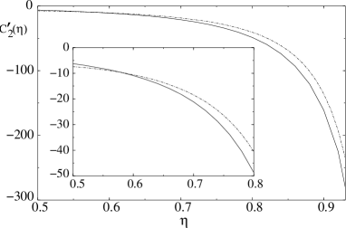
Figure 4: Results for $C^{\prime}_{2}(\eta)$ from VPT: (bold curve) fixed $\omega=0.805$; (dash-dotted) self-consistent determination of $\omega^{\prime}$. Note the divergence as $\eta\to 1$.

Within our approach, the change in the critical particle number is finally obtained as an expansion

$$\frac{1}{\Gamma(\eta-1/2)}I_{\eta}(0)=\zeta(\eta+1)+C_{1}(\eta){\hat{a}}+[C^{\prime}_{1}(\eta)+C^{\prime}_{2}(\eta)]{\hat{a}}^{2\eta}+{\cal O}({\hat{a}}^{2})$$ (45)

with $C_{1}(\eta)$ determined from Eq. (30) and $C^{\prime}_{1}(\eta)=(16\pi)^{\eta}\Gamma(-\eta)$ as in Eq. (39). The coefficient $C^{\prime}_{2}(\eta)$ emerges from VPT. In Fig. 4 we show the VPT calculation for $C^{\prime}_{2}(\eta)$ using the seven-loop data from Ref. Kas03 . The result with self-consistent determination of $\omega^{\prime}$ (bold curve) is compared to the calculation with a fixed value of $\omega^{\prime}=0.805$. We see that both curves agree reasonably well; the calculation of $C^{\prime}_{2}(\eta)$ thus does not depend too sensitively on the exponent. For $\eta\raise 1.29167pt\hbox{$>$\kern-7.5pt\raise-4.73611pt\hbox{$\sim$}}0.94$, the self-consistent calculation of $\omega^{\prime}$ does not converge anymore; one would probably have to extend the resummation to higher orders to resolve this issue. More importantly, however, we see that the results for $C^{\prime}_{2}(\eta)$ diverge in the limit of $\eta\to 1$. This behavior can be traced back to the presence of the $\Gamma$ functions in Eq. (43). The same divergence also appears in the coefficient $C^{\prime}_{1}(\eta)$. We will discuss the significance of these divergences below in connection with the calculation of the critical temperature.

In Fig. 5, we plot the final result, i.e., the shift in the critical temperature, as determined from Eqs. (25) and (45). The figure reflects the characteristic qualitative features discussed in Sec. III and confirms our previous conclusions. The shift is displayed as a function of $\eta$ for a fixed value of ${\hat{a}}=a/\lambda_{T}=10^{-4}$. The full and the dash-dotted curves show the complete result including all terms from Eq. (45). The two curves are respectively based on the calculation of $C^{\prime}_{2}(\eta)$ with $\omega^{\prime}$ kept fixed or determined self-consistently. The discrepancy between these results can be considered an estimate for the error in the calculation of $T_{c}$ that is introduced by the resummation procedure. Since the curves are almost indistinguishable, we can conclude that the resummation contributes only a small inaccuracy in addition to potential further errors introduced by the other approximations.

For the dashed curve in Fig. 5, the term $C^{\prime}_{2}(\eta)\hat{a}^{2\eta}$ has been omitted, it thus displays the mean-field result below second order Zob04 . The dotted curve shows the perturbative contribution due to $C_{1}(\eta)\hat{a}$. We see that the full and the mean-field result closely approach the perturbative first-order approximation long before values of $\eta$ around 1 are reached. The divergence around $\eta=1$ introduced by the behavior of $C_{1}^{\prime}$ and $C_{2}^{\prime}$ is restricted to a very small interval. Thus it is reasonable to expect that the true behavior of $T_{c}$ in this small regime remains well described by the first-order approximation and that the divergence is only an artifact of our calculation. Furthermore, in Ref. Zob04 it was shown that within mean-field theory this divergence is compensated for by a pole in the second-order contribution to the critical particle number. We can also expect the same behavior in the present case, i.e., beyond mean-field theory.

Figure 5: Shift of critical temperature as a function of the potential shape parameter $\eta$ for fixed $a/\lambda_{T}=10^{-4}$: (full curve) Result including all terms in (45) and $C^{\prime}_{2}(\eta)$ calculated with fixed $\omega^{\prime}=0.805$; (dash-dotted) same as full curve but with $\omega^{\prime}$ determined self-consistently; (dashed) $C^{\prime}_{2}(\eta)$ omitted (i.e., “mean-field result”); (dotted) $C^{\prime}_{1}(\eta)$ and $C^{\prime}_{2}(\eta)$ omitted (i.e., only perturbative term).

V Summary and conclusions

We have calculated the shift of the critical temperature of interacting Bose gases trapped in a general power-law potential of the type $\sum_{i}U_{i}|x_{i}|^{p_{i}}$. The objective was to understand how this shift changes when we pass from homogeneous to harmonically trapped systems, interpolating between these limits by changing the power of the potential. While the homogeneous case is influenced strongly by nonperturbative critical fluctuations, the harmonic case can be calculated perturbatively.

We have restricted our attention to the thermodynamic limit, which allowed us to use the local-density approximation in which the Bose gas is assumed to be locally homogeneous at each point. In Sec. III, we gave justification for this procedure. The main result is the shift formula

$$\frac{T_{c}-T_{c}^{0}}{T_{c}^{0}}=D_{1}(\eta)\frac{a}{\lambda_{T}}+D^{\prime}(\eta)\left(\frac{a}{\lambda_{T}}\right)^{2\eta}+{\cal O}(a^{2}).$$ (46)

It contains a linear, perturbative part, which is relevant for all potentials, and a nonperturbative contribution proportional to $(a/\lambda_{T})^{2\eta}$. For small $a/\lambda_{T}$, the latter contributes significantly only in the quasihomogeneous regime.

The presence of the $(a/\lambda_{T})^{2\eta}$ term was derived from scaling and resummation arguments, and we gave a simple physical explanation for its appearance based on the Ginzburg criterion GI . Our results show how the growing inhomogeneity of the potential reduces the significance of critical fluctuations.

We also performed an explicit calculation of the nonperturbative coefficient $D^{\prime}(\eta)$. In spite of the approximate character of the calculation, the result should be quite accurate. Our approach was based on the resummation of divergent perturbation series with the help of field-theoretic variational perturbation theory. In the course of the derivation, it was shown that the simple Hartree-Fock approximation also contains a nonperturbative contribution.

Finally, our study indicates that the higher-order $T_{c}$ shift in traps with $\eta=1$, for instance in $\sum_{i}U|x_{i}|^{6}$ potentials, should be particularly interesting and difficult to investigate. In the limit $\eta\rightarrow 1$, we find a divergence in the coefficient $D^{\prime}(\eta)$ which governs the nonperturbative contribution proportional to $(a/\lambda_{T})^{2}$. It remains to be investigated whether this divergence is canceled by other genuinely second-order terms, as it is expected from mean-field theory. For future work, it might also be of interest to study the influence of other types of external potentials on the transition temperature, such as optical lattices KleSchPel04 .

- (1) G. Baym, J.-P. Blaizot, M. Holzmann, F. Laloë, and D. Vautherin, Phys. Rev. Lett. 83, 1703 (1999).
- (2) P. Arnold, G. Moore, and B. Tomásik, Phys. Rev. A 65, 013606 (2001).
- (3) V. A. Kashurnikov, N. V. Prokof’ev, and B. V. Svistunov, Phys. Rev. Lett. 87, 120402 (2001).
- (4) P. Arnold and G. Moore, Phys. Rev. Lett. 87, 120401 (2001).
- (5) S. Giorgini, L. P. Pitaevskii, and S. Stringari, Phys. Rev. A 54, R4633 (1996).
- (6) P. Arnold and B. Tomásik, Phys. Rev. A 64, 053609 (2001).
- (7) O. Zobay, J. Phys. B 37, 2593 (2004).
- (8) O. Zobay, G. Metikas, and G. Alber, Phys. Rev. A 69, 063615 (2004).
- (9) H. Shi and W.-M. Zheng, Phys. Rev. A 56, 1046 (1997).
- (10) H. Kleinert, Path Integrals in Quantum Mechanics, Statistics, Polymer Physics, and Financial Markets, 3rd ed. (World Scientific, Singapore, 2004); http://www.physik.fu-berlin.de/~kleinert/b8
- (11) G. Metikas, O. Zobay, and G. Alber, Phys. Rev. A 69, 043614 (2004).
- (12) H. Kleinert, Phys. Rev. D 57, 2264 (1998); 58, 107702A (1998) (cond-mat/9803268); Phys. Lett. B 434, 74 (1998) (cond-mat/9801167).
- (13) H. Kleinert and V. Schulte-Frohlinde, Critical Properties of -Theories (World Scientific, Singapore, 2001).
- (14) H. Kleinert, Phys. Rev. D 60, 085001 (1999) (hep-th/9812197).
- (15) J. A. Lipa, J. A. Nissen, D. A. Stricker, D. R. Swanson, and T. C. P. Chui, Phys. Rev. B 68, 174518 (2003).
- (16) H. Kleinert, Mod. Phys. Lett. B 17, 1011 (2003).
- (17) B. Kastening, Phys. Rev. A 68, 061601(R) (2003); 69, 043613 (2004); 70, 043621 (2004); Laser Phys. 14, 586, (2004).
- (18) J. Zinn-Justin, Quantum Field Theory and Critical Phenomena (Oxford University Press, Oxford, 1989).
- (19) R. P. Feynman and H. Kleinert, Phys. Rev. A 34, 5080 (1986).
- (20) V.L. Ginzburg, Fiz. Twerd. Tela (Leningrad) 2, 2031 (1960) [Sov. Phys. Solid State 2, 1824 (1961)]; see also the detailed discussion in Chapter 13 of the textbook L.D. Landau and E.M. Lifshitz, Statistical Physics, 3rd ed. (Pergamon, London, 1968). Strictly speaking, the onset of fluctuations in a complex U(1)-symmetric field theory is not determined by Ginzburg’s criterion which concerns only size fluctuations, but by a modification of it concerning the much more relevant phase fluctuations; see H. Kleinert, Phys. Rev. Lett. 84, 286 (2000).
- (21) V. Bagnato, D. E. Pritchard, and D. Kleppner, Phys. Rev. A 35, 4354 (1987).
- (22) M. Li, L. Chen, and C. Chen, Phys. Rev. A 59, 3109 (1999).
- (23) Z. Yan, Phys. Rev. A 61, 063607 (2000).
- (24) For detailed properties see Chapter 7 in PI .
- (25) M. Holzmann, G. Baym, J.-P. Blaizot, and F. Laloë, Phys. Rev. Lett. 87, 120403 (2001).
- (26) A. L. Fetter and J. D. Walecka, Quantum Theory of Many-Particle Systems (McGraw-Hill, New York, 1971).
- (27) J. E. Robinson, Phys. Rev. 83, 678 (1951).
- (28) H. Kleinert, S. Schmidt, and A. Pelster, Phys. Rev. Lett. 93, 160402 (2004).