Non-universal coarsening and universal distributions in far-from equilibrium systems

Abstract

Anomalous coarsening in far-from equilibrium one-dimensional systems is investigated by applying simulation and analytic techniques to minimal hard core particle (exclusion) models. They contain mechanisms of aggregated particle diffusion, with rates $\epsilon\ll 1$, particle deposition into cluster gaps, but suppressed for the smallest gaps, and breakup of clusters which are adjacent to large gaps. Cluster breakup rates vary with the cluster length $x$ as $kx^{\alpha}$. The domain growth law $\langle x\rangle\sim{\left(\epsilon t\right)}^{z}$, with $z=1/\left(2+\alpha\right)$ for $\alpha>0$, is explained by a simple scaling picture involving the time for two particles to coalesce and a new particle be deposited. The density of double vacancies, at which deposition and cluster breakup are allowed, scale as $1/\left[t{\left(\epsilon t\right)}^{z}\right]$. Numerical simulations for several values of $\alpha$ and $\epsilon$ confirm these results. A fuller approach is presented which employs a mapping of cluster configurations to a column picture and an approximate factorization of the cluster configuration probability within the resulting master equation. The equation for a one-variable scaling function explains the above average cluster length scaling. The probability distributions of cluster lengths $x$ scale as $P(x)=\frac{1}{{\left(\epsilon t\right)}^{z}}g(y)$, with $y\equiv x/{\left(\epsilon t\right)}^{z}$, which is confirmed by simulation. However, those distributions show a universal tail with the form $g(y)\sim\exp{\left(-y^{3/2}\right)}$, which is explained by the connection of the vacancy dynamics with the problem of particle trapping in an infinite sea of traps. The high correlations of surviving particle displacement in the latter problem explains the failure of the independent cluster approximation to represent those rare events.

I Introduction

Domain growth in far from equilibrium systems is a subject of increasing interest due to the large number of applications, such as phase separation of mixtures, dynamics of glasses and island coarsening after thin film deposition [2, 3, 1]. In these systems, their dynamics is responsible for bringing them to steady states, while external agents act to drive them out of equilibrium. Many statistical models exhibit simple, universal domain growth laws, which are found in some real systems, but there is much interest in models with slow coarsening and with continuously varying growth exponents, for instance due to their potential applications to glassy systems [2, 3, 4].

In this paper, we will consider one-dimensional models with particle deposition and diffusion, reversible aggregation to clusters and mechanisms of cluster breaking which show such a variety of domain growth laws. Cluster breaking may be an effect of internal stress and was previously considered in studies of island growth in submonolayers [5]. In a real system subject to external pressure but with some type of geometrical frustration other than those observed in island growth, it is expected that cluster breaking will compete with mechanisms of densification, these ones to be represented by vacancy filling (deposition of new particles). However, the onset of those processes depends on the formation of large vacancies due to the (slow) diffusion of aggregated particles. The coarsening exponents of those systems will be shown to vary with the exponents in the scaling of the cluster break probabilities, although the cluster lengths distributions are universal. Consequently, these one-dimensional statistical models, although not related to a specific real problem, reveal some interesting features that may help to understand complex three-dimensional systems, with the advantage of being more tractable both analytically and numerically.

The models presented here are nontrivial extensions of those analyzed in a recent paper [6], which include particle diffusion, reversible aggregation to clusters and deposition mechanisms. In the original model, hard-core particles in a one-dimensional lattice have diffusion rates $r=d$ when they were free (i. e., they have two empty nearest-neighbor sites) and $r=\epsilon\sim e^{-E/T}$ when they have one occupied nearest neighbor site, with $r\ll d$ (Fig. 1a). The deposition rate is $F=1$, in units of monolayers per time step, and is restricted to sites with at least one empty nearest neighbor (Fig. 1b), i. e. a site of a double or larger vacancy. These dynamical rules were motivated by the Clarke-Vvedensky model and related models of thin films or submonolayer growth [7], but included effects of geometrical frustration that forbid filling of single vacancies. Domain growth in the form $\langle d\rangle\sim\epsilon^{-1/2}t^{1/2}$ was predicted analytically and from simulation [6]. The same model without deposition and in the limit $\epsilon\ll 1$ showed domain growth as $t^{1/3}$ before approaching a steady state [6].

Here, in addition to the processes of the original model (Figs. 1a and 1b), we will consider the competition between deposition of new particles and the breaking of a neighboring cluster when a double (or larger) vacancy appears. In this model, a cluster of length $x$ with two vacancies at one of its sides (where deposition may also occur) may break in two pieces, at a random internal position, with rate $kx^{\alpha}$, where the exponent $\alpha$ is a tunable parameter and $k$ is a constant amplitude. The process is illustrated in Fig. 1c for a cluster with $x=6$, with a total of $5$ internal points for its separation into two pieces. Our focus is the non-trivial case $\alpha>0$, for which $\alpha$-dependent coarsening exponents are obtained.

Notice that this model is significantly different from other models which involve coagulation or breakup of clusters with size-dependent rates with variable exponents [8, 9, 10, 11]. Here, the clusters slowly gain mass by (non-biased) diffusion at the expense of neighboring clusters, while breakup is subject to the availability of free space for its expansion.

Scaling laws for the average cluster length $\langle x\rangle$ in the form

$$\langle x\rangle\sim t^{z}$$ (1)

will be obtained, where $z$ is called the coarsening exponent. In the models with the cluster breaking mechanism, the exponent $z$ can be continuously tuned from $0$ to $1/2$ by varying the scaling exponent $\alpha$ of the rate of cluster breaking. This result is predicted by a scaling theory that also described the cluster growth laws of Ref. [6] and is confirmed by numerical simulations with very good accuracy. It is also possible to describe such systems in terms of interval probabilities, which allows the analytic investigation based on an independent cluster approximation. Using this method, we also predict the coarsening exponents of the model.

There is also much interest in knowing the distributions of cluster lengths in such anomalously growing systems. Those distributions are also calculated numerically and show an universal ($\alpha$-independent) form $P\left(x\right)\sim\exp{\left(-x^{3/2}\right)}$, despite the fact that the coarsening exponents do depend on $\alpha$. The analytical treatment of the model in the independent cluster approximation gives instead an $\alpha$-dependent power in the exponent ($-x^{1+\alpha/2}$). However, it can be shown that the dynamics of large clusters is related to the problem of particle diffusion in an infinite sea of mobile traps [12, 13, 14], where the holes between clusters in the former problem correspond to the particles in the latter. This connection leads to the above universal cluster length distribution and explains the failure of the independent cluster approximation to predict those distributions.

This paper is organized as follows. In Sec. II we present the scaling theory and obtain the coarsening exponents. In Sec. III we present the results of simulations for the time dependence of average cluster lengths and density of double vacancies. In Sec. IV, we map the cluster configurations to a column picture and determine the master equation with the independent interval approximation to the joint cluster length probability. In Sec. V, we discuss the cluster length probabilities, comparing numerical results, the analytical prediction of the independent interval approximation and the connection to the problem of one diffusing particle in a sea of moving traps. In Sec. VI, we summarize our results and present our conclusions.

II Models and scaling theories

Here we will define our models and estimate coarsening exponents using scaling arguments along the lines of Ref. [6], which were previously adopted in the analysis of related systems by Evans [3] and introduced in the analysis of domain growth in magnetic systems by Lai et al [15] and Shore et al [16].

First we consider the original model of deposition and diffusion presented in Ref. [6] (Figs. 1a and 1b).

For simplicity, we will refer to the average cluster length as $x$. In Fig. 2a, we show a configuration with clusters of lengths typically of order $x$, named $A$, $B$ and $C$, with single empty sites (single vacancies) between them. Deposition is not allowed at those vacancies, as well as at the other single holes separating $A$ and $C$ from other neighboring clusters. Suppose that the length of $A$ tends to increase in time, while the length of $B$ decreases, as shown in Fig. 2b. This evolution is equivalent to the diffusion of the vacancy between $A$ and $B$, which gets closer to the vacancy between $B$ and $C$ (diffusion of this vacancy was not shown only to simplify the illustration). Finally, the length of $A$ will increase by $x$ when $A$ and $B$ coalesce, as shown in Fig. 2c. At that time, a new particle is deposited in an empty site of the double vacancy, which is also shown in Fig. 2c.

The deposition process occurred after all particles of cluster $B$ have detached from it and aggregated to cluster $A$. This is equivalent to displacement of order $x$ of the diffusing vacancy between $A$ and $B$. Notice that in a configuration with two neighboring empty sites (Fig. 2c), the probability of deposition (fixed rate $F=1$) is much larger than the probability of diffusion of an aggregated particle ($\epsilon\ll 1$), thus it is highly improbable that a diffusion process will follow the formation of a double vacancy. Consequently, the time necessary for coarsening of two clusters of length $x$ is of the order of the time for a diffusing vacancy to move a distance $x$, which is $\Delta t\sim{\epsilon}^{-1}x^{2}$. In the configuration after deposition, the average cluster length is increased by $x$, since it was equivalent to the merging of cluster $B$ into cluster $A$. Consequently, the average cluster length increases as

$${{dx}\over{dt}}\sim{{\Delta x}\over{\Delta t}}\sim{x\over{{\epsilon}^{-1}x^{2}}}={\epsilon\over x}.$$ (2)

Integrating Eq. 2, we obtain $x\sim{\epsilon}^{1/2}t^{1/2}$, in agreement with the analytical results of the independent cluster approximation and simulation data [6].

Now consider the problem with the cluster breaking mechanism. It is assumed that a cluster of length $x$ breaks with rate

$$r_{cb}=kx^{\alpha}$$ (3)

only when there is enough space available, i. e., when there is more than one empty site at one of the sides of the cluster. This process is illustrated in Fig. 1c, in which a cluster of length $x=6$ may break at five different internal points, which gives five possible final configurations if the breaking occurs - three of them were shown in Fig. 1c.

Following the argument of the original model, after the diffusion processes leading to the onset of a double vacancy (Fig. 2c), there are three possibilities: a) a new particle is deposited with rate $F=1$; b) the cluster at the right side of the double vacancy breaks; c) the cluster at the left side breaks. Since the two neighboring clusters have lengths of order $x$, deposition will occur with probability $P_{dep}\sim 1/x^{\alpha}$ for $\alpha>0$ and $x\ll 1$. Otherwise, one of the clusters adjacent to the double vacancy will break in two pieces.

If a new particle is deposited, then the average cluster length will increase by $x$, such as in model I. On the other hand, in the most probable case of an adjacent cluster to break, the average cluster length will not increase. Consequently, the average cluster length increases as

$${{dx}\over{dt}}\sim P_{dep}{{\Delta x}\over{\Delta t}}\sim\frac{1}{x^{\alpha}}\frac{x}{{\epsilon}^{-1}x^{2}}={\epsilon\over x^{1+\alpha}}.$$ (4)

Integrating Eq. 4, we obtain

$$x\sim{\epsilon t}^{z},z={1\over{2+\alpha}}.$$ (5)

For $\alpha<0$, the above reasoning leads to $P_{dep}\approx 1$ for large $x$ and, consequently, $z=1/2$, as in the original model.

For $\alpha>0$, Eq. 5 shows that the coarsening exponent can be continuously tuned from $z=0$ to $z=0.5$ by changing the cluster breaking exponent.

The same arguments can be used to predict the density of double vacancies, $\rho_{00}\left(t\right)$, a quantity which plays a important role in the analytic calculations of Sec. IV. The total rate at which deposition and cluster-breaking occur after the formation of a double vacancy (Fig. 2c) is of order $x^{\alpha}$, for $\alpha>0$. Consequently, that vacancy will survive during a time $1/x^{\alpha}$, while it takes a time of order $\Delta t\sim{\epsilon}^{-1}x^{2}$ to be formed (Figs. 2a-2c). Consequently, one double vacancy between two clusters of length $x$ typically survives during a fraction ${\left(1/x^{\alpha}\right)}/{\left({\epsilon}^{-1}x^{2}\right)}$ of the total time. To obtain its density we must divide this quantity by the average cluster length $x$, which gives

$$\rho_{00}\left(t\right)\sim\frac{\left(1/x^{\alpha}\right)}{\left({\epsilon}^{-1}x^{2}\right)}\frac{1}{x}\sim{\epsilon\over x^{3+\alpha}}\sim{{\epsilon t}^{-z}\over{t}}.$$ (6)

Notice that this time decay does not involve the diffusive factor $\epsilon t$ alone.

III Simulation results for average lengths and densities

We simulated the model for cluster-breaking exponents $\alpha=0.5$, $\alpha=1$, $\alpha=2$ and $\alpha=4$, with $\epsilon=0.001$ and, in some cases, also with $\epsilon=0.01$. Deposition rates, free particle diffusion rates and amplitudes of cluster breaking rates were $F=1$, $d=1$ and $k=1$, respectively, in all simulations. Lattices lengths were $L=5\times{10}^{4}$. The maximum simulation times were ${10}^{6}$ for the smaller value of $\alpha$ and ${10}^{8}$ for the largest one. Thus, at all times, the whole lattice contained more than $500$ clusters, which was essential to avoid finite-size effects. Indeed, several results were compared with those in lattices of lengths $L={10}^{4}$ and confirmed the absence of significant finite-size effects. The number of different realizations varied from $5000$ for the smaller $\alpha$ to $500$ for the largest one.

The scaling of the average cluster length $\langle x\rangle$ on $\epsilon$ and $t$ is confirmed in Fig. 3 for $\alpha=1$, by showing $\langle x\rangle/{\left(\epsilon t\right)}^{1/3}$ for $\epsilon=0.01$ and $\epsilon=0.001$ as a function of $1/{\left(\epsilon t\right)}^{1/3}$. The data collapse confirms the expected scaling on $\epsilon$, the convergence to a finite value as $t\to\infty$ confirms the scaling on $t$ and the variable in the abscissa suggests a constant correction term to Eq. (4).

In Fig. 4a and 4b we show $\langle x\rangle/{\left(\epsilon t\right)}^{z}$ versus $1/{\left(\epsilon t\right)}^{z}$ for $\alpha=0.5$ and $\alpha=2$, respectively, with the values of $z$ given by Eq. (4) and $\epsilon=0.001$. These results confirm the validity of the scaling theory of Sec. II for the average cluster length.

Since double vacancies are very rare, the accuracy of their density is much lower than the accuracy of $\langle x\rangle$. Consequently, averages over relatively large time regions were necessary to study the long time evolution of that density. The average values agree with the predicted scaling (Eq. 6), as shown in Fig. 5 for $\alpha=1$ (with two values of $\epsilon$). Notice that the different time and $\epsilon$ dependences were confirmed there.

IV Theoretical analysis under the independent cluster approximation

Now we turn next to the more powerful analysis starting from a version of the master equation, which can provide a full description of the process. This is more easily set up by reformulating the process using a column picture, in which a column of height $m$ represents a cluster of size $m$. The map of the problem of particles in a line onto the cluster problem in a line of reduced length is shown in Figs. 6a and 6b. The original diffusion processes of free and aggregated particles correspond to those shown in Fig. 6b. Since one cluster has two edges but corresponds to a single column, the one-particle detachment rate in the column picture is

$$\gamma=2\epsilon.$$ (7)

Finally, in Fig. 7 we illustrate the competition between deposition of a new particle and cluster breaking after the formation of a double vacancy in the particle picture, which corresponds to the formation of a single vacancy in the cluster picture.

The deposition process (Fig. 7) leads to the decrease of the total number of clusters and of the number of holes between the clusters as time increases. On the other hand, the length $L$ of the line in which particles are deposited and diffuse is kept constant. Consequently, in order to adopt the column picture, it is necessary to consider that the length $L_{0}$ of the corresponding column problem decreases in time. These lengths are related as $L_{0}=L-M$, where $M$ is the total mass or total number of particles, for periodic boundary conditions.

We denote by $P_{t}(m)$ the probability that a randomly chosen cluster (equivalently, column) has size $m$ at time $t$. It is given in terms of the clusters numbers $N(m,t)$ by

$$P_{t}(m)={{N(m,t)}\over{L_{0}(t)}},$$ (8)

while the length of the lattice in which the column problem is defined varies due to deposition as

$${{L_{0}(t+1)-L_{0}(t)}\over{L_{0}(t)}}=-P_{t}(0)\left[2-P_{t}(0)\right].$$ (9)

Here, $P_{t}(0)$ is the probability of an empty site in the column problem, which correspond to double vacancies in the original particle problem (see Figs. 6 and 7).

Then the gain/loss from in/out processes provides a master equation which must be written in terms of clusters numbers $N(m,t)$ in the general form

$$N(m,t+1)-N(m,t)=L_{0}\left(B_{m}+C_{m}+D_{m}+{\cal B}_{m}\right),$$ (10)

where $B_{m}$ comes from the cluster breaking processes, $C_{m}$ comes from the diffusion of aggregated particles (detachment of particles from clusters), $D_{m}$ comes from the diffusion of free particles and ${\cal B}_{m}$ comes from the deposition processes. The terms in the right-hand side of Eq. (10) are thus written in terms of probabilities of cluster masses at time $t$.

In an independent interval approximation in which joint probabilities are factorized, they are given by

$$C_{m} = \gamma\theta(m+1-2)P_{t}(m+1)+\gamma\theta(m-1)P_{t}(m-1)\left[1-P_{t}(0)-P_{t}(1)\right]$$ (12)

$$-\gamma\theta(m-2)P_{t}(m)-\gamma P_{t}(m)\left[1-P_{t}(0)-P_{t}(1)\right],$$

$$D_{m} = d\theta(m-1)P_{t}(m-1)P_{t}(1)+d\delta_{m,0}P_{t}(1)-d\delta_{m,1}P_{t}(1)-dP_{t}(m)P_{t}(1)$$ (13)

$$= dP_{t}(1)\left[\theta(m-1)P_{t}(m-1)+\delta_{m,0}-\delta_{m,1}-P_{t}(m)\right],$$ (14)

$${\cal B}_{m}=P_{t}(0)\left[2\theta\left(m-2\right)P_{t}\left(m-1\right)-2\theta\left(m-1\right)P_{t}\left(m\right)+\delta_{m,1}P_{t}\left(0\right)-2\delta_{m,0}\right]$$ (15)

and

$$B_{m} = 2\theta(m-1)P_{t}(0)\sum_{r=1}^{\infty}{f(m+r)P_{t}(m+r)}$$ (17)

$$-\theta(m-2)f(m)P_{t}(m)(m-1)P_{t}(0)-\delta_{m,0}P_{t}(0)\sum_{p=2}^{\infty}{(p-1)f(p)P_{t}(p)}$$

$$= P_{t}(0)[2\theta(m-1)\sum_{r=1}^{\infty}{f(m+r)P_{t}(m+r)}$$ (19)

$$-\theta(m-2)(m-1)f(m)P_{t}(m)-\delta_{m,0}\sum_{p=2}^{\infty}{(p-1)f(p)P_{t}(p)}].$$

In Eq. (19), the function $f(m)$ gives the rate for a cluster of mass $m$ to break at each internal point, i. e. at each internal connection between two aggregated particles:

$$f(m)=k\frac{{\left(m-1\right)}^{\alpha}}{m-1}=k{\left(m-1\right)}^{\alpha-1}.$$ (20)

The generating function

$$G_{t}(s)\equiv\sum_{m=0}^{\infty}{P_{t}(m)s^{m}}$$ (21)

satisfies

$$G_{t+1}(s){\left[1-P_{t}(0)\right]}^{2}-G_{t}(s)={\cal L}\left(B+C+D+{\cal B}\right),$$ (22)

where the operator ${\cal L}$ is defined as

$${\cal L}g=\sum_{m=0}^{\infty}{g(m)s^{m}}.$$ (23)

We thus obtain

$${\cal L}C={\gamma\over s}\left(1-s\right)\left[G_{t}(s)-P_{t}(0)-P_{t}(1)s\right]+\left(s-1\right)\gamma bG_{t}(s),$$ (24)

with

$$b\equiv 1-P_{t}(0)-P_{t}(1),$$ (25)

$${\cal L}D=dP_{t}(1)\left(s-1\right)\left[G_{t}(s)-1\right],$$ (26)

$${\cal L}{\cal B}=P_{t}(0)\left[2\left(s-1\right)\left(G_{t}(s)-P_{t}(0)\right)+sP_{t}(0)-2\right]$$ (27)

and

$${\cal L}B = 2P_{t}(0)\sum_{m=1}^{\infty}{\left[s^{m}\sum_{r=0}^{\infty}{f(m+r)P_{t}(m+r)}\right]}-P_{t}(0)\sum_{m=2}^{\infty}{s^{m}\left(m-1\right)f(m)P_{t}(m)}$$ (29)

$$-P_{t}(0)\sum_{m=2}^{\infty}{\left(p-1\right)f(p)P_{t}(p)}.$$

Eqs. (24), (26) and (27) are the same obtained in Ref. [6] for the model with only deposition and diffusion (with $d=1$).

Now defining the operator ${\cal F}$ so that

$${\cal F}\left(s{\partial\over{\partial s}}\right)\sum_{m}{e^{sm}g(m)}=\sum_{m}{f(m)e^{sm}g(m)},$$ (30)

we may write the contribution of cluster breaking processes to the generating function as

$${\cal L}B = P_{t}(0)\frac{\left(1+s\right)}{\left(1-s\right)}\left[{\left[{\cal F}\left(s{\partial\over{\partial s}}\right)G_{t}(s)\right]}_{s=1}-{\cal F}\left(s{\partial\over{\partial s}}\right)G_{t}(s)\right]$$ (32)

$$-P_{t}(0)\left[{\left[s{\partial\over{\partial s}}{\cal F}\left(s{\partial\over{\partial s}}\right)G_{t}(s)\right]}_{s=1}+s{\partial\over{\partial s}}{\cal F}\left(s{\partial\over{\partial s}}\right)G_{t}(s)\right].$$

Because deposition slowly fills the system, we expect the configurations to coarsen and presumably to go into some scaling asymptotics where mass scales with some power of $t$, and $P_{t}(m)$ and $G_{t}(s)$ each become one-variable scaling functions. So we look for a long time scaling solution of the above equation, in which the finite difference $G_{t+1}(s)-G_{t}(s)$ in Eq. (22) can be taken as a time derivative. The scaling variable will be some combination of $t$ (large) and $u\equiv 1-s$ (small), the latter because large cluster sizes arise from structure in $G_{t}(s)$ at $s\approx 1$. The variable $u$ is actually conjugate to $m$. Coarsening will correspond to the scale of $m$ as $t^{z}$, with some power $z$, in which case the one-variable form will be

$$G_{t}(s)=u^{\alpha}F\left(ut^{z}\right),$$ (33)

with some function $F$. Normalization requires $\alpha=0$ and $F(0)=1$. In the scaling limit, the relationship of the generating function to the probability $P_{t}(m)$ requires the latter to be of the form

$$P_{t}(m)={1\over{t^{z}}}g\left({m\over{t^{z}}}\right),$$ (34)

with

$$F(x)=\int_{0}^{\infty}{g(y)e^{-xy}dy}.$$ (35)

Moreover, for $s\approx 1$ one has $s{\partial\over{\partial s}}\approx{\partial\over{\partial u}}$ in Eq. (32).

Thus we obtain the following equation for the one-variable scaling function:

$$\left[{\left(1-\frac{1}{t^{z}}g(0)\right)}^{2}\left(1+{\partial\over{\partial t}}\right)-1\right]F{\left(ut^{z}\right)}=$$ (41)

$$\begin{array}[]{r}u\left[F{\left(ut^{z}\right)}\left(a-\gamma\left(1-u+u^{2}+\dots\right)\right)+\left(\gamma-1\right)\frac{1}{t^{z}}g{\left(\frac{1}{t^{z}}\right)}+\gamma\left(1-u+u^{2}+\dots\right)\frac{1}{t^{z}}g(0)\right]\\ +\frac{1}{t^{z}}g(0)\left[2uF{\left(ut^{z}\right)}-\left(1-u\right)\frac{1}{t^{z}}g(0)+\frac{2}{t^{z}}g(0)-2\right]\\ +\frac{1}{t^{z}}g(0)\left[-\frac{\left(2+u\right)}{u}{\left[{\cal F}\left({\partial\over{\partial u}}\right)F{\left(ut^{z}\right)}\right]}_{u=0}-{\left[{\partial\over{\partial u}}{\cal F}\left({\partial\over{\partial u}}\right)F{\left(ut^{z}\right)}\right]}_{u=0}\right]\\ -\frac{1}{t^{z}}g(0)\left({\partial\over{\partial u}}-\frac{\left(2+u\right)}{u}\right)F{\left(ut^{z}\right)},\end{array}$$

where $a\equiv\gamma-\gamma P_{t}(0)+\left(1-\gamma\right)P_{t}(1)$.

The dominant terms in Eq. 41 give

$$\frac{zx}{t}F^{\prime}(x)-2P_{t}(0)F(x) = \gamma{\left(\frac{x}{t^{z}}\right)}^{2}F(x)-2P_{t}(0)$$ (44)

$$+P_{t}(0)t^{z}\left[-\frac{2}{x}{\left[{\cal F}\left(t^{z}\frac{d}{dx}\right)F(x)\right]}_{x=0}-{\left[\frac{d}{dx}{\cal F}\left(t^{z}\frac{d}{dx}\right)F(x)\right]}_{x=0}\right]$$

$$+P_{t}(0)t^{z}\left(\frac{2}{x}-\frac{d}{dx}\right){\cal F}\left(t^{z}\frac{d}{dx}\right)F(x).$$

In the scaling limit, the first term at the left hand side (LHS) is of order $1/t$. Assuming that the density of clusters of zero mass (holes in the column picture) decays as

$$P_{t}(0)\sim\frac{1}{t^{\beta}},$$ (45)

the second term at the LHS and the second term at the right hand side (RHS) of Eq. (44) are both of order $1/t^{\beta}$. The first term in the RHS, related to the diffusion of aggregated particles, is of order $1/t^{2z}$. Since cluster breaking competes with deposition and recalling that the coarsening exponent in the problem with only deposition and diffusion is $z=1/2$, we expect that, in the present system, $z\leq 1/2$ for any $\alpha$. The last term in the RHS, associated with cluster breaking, is of order $1/t^{\left(\beta-z\alpha\right)}$, which clearly dominates over the terms which scale as $1/t^{\beta}$ for any $\alpha>0$. Thus, we conclude that the terms associated with aggregated particles diffusion (first of the RHS of Eq. 44) and with cluster breaking (last of the RHS) are dominant for $\alpha>0$ and must cancel each other, while the remaining terms are subdominant contribution which must also cancel. From the dominant terms, we obtain

$$2z=\beta-z\alpha$$ (46)

and from the subdominant terms we obtain

$$\beta=1,$$ (47)

which gives the coarsening exponent

$$z=1/\left(2+\alpha\right).$$ (48)

The value of $z$ agrees with that obtained from scaling arguments and in simulations. In order to compare the density of single vacancies in the column problem, $P_{t}(0)$, and the density of double vacancies in the original particle problem, $\rho_{00}\left(t\right)$, we consider that the total length of the lattice in the column problem, $L_{0}$, is smaller than the length $L$ by a factor of the order of the average cluster size (see Figs. 6 and 7), which scales as $t^{z}$. Consequently

$$\rho_{00}\left(t\right)\sim P_{t}(0)/t^{z}\sim t^{-\left(1+z\right)},$$ (49)

which also agrees with the scaling arguments of Sec. II and simulation results. The $\epsilon$- or $\gamma$-dependence of average cluster size and densities of vacancies in both pictures, predicted in Secs. II and III, also follow from Eq. (44).

Also notice that, for $\alpha<0$, the cluster breaking term of Eq. (44) is not dominant anymore and we obtain $z=1/2$, as in the problem without that mechanism (Ref. [6]).

V Distributions of cluster lengths

An equation for the one-variable scaling function $F(x)$ follows from the balance of the dominant terms in Eq. (44), related to diffusion of aggregated particles and cluster breaking:

$$\frac{\gamma x^{2}F(x)}{t^{2z}} = P_{t}(0)t^{z}\left[\frac{2}{x}{\left[{\cal F}\left(-t^{z}\frac{d}{dx}\right)F(x)\right]}_{x=0}+{\left[\frac{d}{dx}{\cal F}\left(-t^{z}\frac{d}{dx}\right)F(x)\right]}_{x=0}\right]$$ (51)

$$+P_{t}(0)t^{z}\left(\frac{d}{dx}-\frac{2}{x}\right){\cal F}\left(-t^{z}\frac{d}{dx}\right)F(x)$$

Physically, it means that the dynamics in long time regime is dominated by diffusion of aggregated particles, which forms larger clusters at the expenses of neighboring ones, and cluster breaking, which restores a relatively random size distribution after the onset of a vacancy in the column picture (double vacancy in the particle picture). Deposition becomes a rare process, as expected with the large probabilities of cluster breaking for $\alpha>0$, and does not contribute to determine the main features of the scaling function.

Instead of solving Eq. (51) for the function $F(x)$, which would involve fractional derivatives for non-integer exponents $\alpha$, we consider the same balance of contributions of diffusion of aggregated particles and cluster breaking in the original master equation (10), (12) and (19). They can be rewritten in terms of the function $g(y)$ defined in Eq. (34). At this point, we must consider that $P_{t}(0)$ scales as

$$P_{t}(0)\approx\frac{\left(k_{0}/k\right)}{t},$$ (52)

where $k_{0}\sim{\it o}(1)$, since the survival time of those vacancies is inversely proportional to the amplitude $k$ of the rate of cluster breaking (Eq. 3). We are thus led to

$$\frac{\gamma}{t^{2z}}\frac{d^{2}g(y)}{dy^{2}}+\frac{\left(k_{0}/k\right)}{t}t^{z}kt^{z\left(\alpha-1\right)}\left[2\int_{y}^{\infty}{dy^{\prime}{y^{\prime}}^{\left(\alpha-1\right)}g(y^{\prime})}-y^{\alpha}g(y)-\delta(y)\int_{0}^{\infty}{dy^{\prime}{y^{\prime}}^{\left(\alpha-1\right)}g(y^{\prime})}\right]$$ (53)

$$=0.$$ (54)

For $y>0$, Eq. (54) leads to

$$\gamma_{1}g^{\prime\prime\prime}=y^{\alpha}g^{\prime}+\left(2+\alpha\right)y^{\alpha-1}g,$$ (55)

with $\gamma_{1}=\gamma/k_{0}$. From this equation we obtain the distribution in the form

$$g(y)\sim y^{\mu}\exp{\left(-Ay^{\nu}\right)},$$ (56)

with

$$\nu=1+\alpha/2,\mu=1-\alpha/4,A\sim{\gamma}^{-1/2},$$ (57)

which suggests that the shapes of the distributions of cluster lengths also depend on the cluster breaking exponents.

This prediction can be compared with simulation results. In all cases, the distributions were obtained by taking the length of each cluster only once while spanning the lattice at a fixed simulation time. Thus our estimates can be directly compared with the predictions from the column picture. On the other hand, if a site average had been done during the simulations, a rescaling of the predictions of the column picture would be necessary.

In Figs. 8a and 8b we show the scaled cluster length distributions for $\alpha=2$ and $\alpha=4$, respectively. From Eqs. (56) and (57), it is expected that $\ln{\left[{\left(\epsilon t\right)}^{z}P_{t}(m)/y^{\mu}\right]}$ decreases linearly with $y^{\nu}$, with

$$y\equiv m/{\left(\epsilon t\right)}^{z}$$ (58)

($\mu=1/2$ and $\nu=2$ for $\alpha=2$, $\mu=0$ and $\nu=3$ for $\alpha=4$). Here a factor $\epsilon^{-z}$ multiplies the variable in Eq. (34).

However, the curved shapes of the plots in Figs. 8a and 8b disagree with the predictions of this independent cluster approximation. On the other hand, it was observed that the data for all values of $\alpha$ can be fitted by a universal distribution of the form

$$g(y)\equiv{\left(\epsilon t\right)}^{z}P_{t}(m)\sim\exp{\left(-y^{3/2}\right)}.$$ (59)

This is illustrated in Figs. 9a and 9b for $\alpha=0.5$ and $\alpha=1$, respectively, in which the deviations from Eqs. (56) and (57) are relatively small (indeed, for $\alpha=1$, the exponent $3/2$ of the universal distribution is also predicted by Eq. 57), and in Figs. 10a and 10b for $\alpha=2$ and $\alpha=4$, respectively. Least squares fits of the data for the largest lengths (dashed lines shifted two units to the right in Figs. 9 and 10) confirm the validity of this universal scaling.

In order to explain this unexpected result, we must pay attention to the details of the dynamical process during the coarsening process, which comes from a balance between aggregated particle diffusion and cluster breaking, and its connection to diffusion-reaction related problems. Turning back to the original particle picture of the problem, during almost all the time, the dynamics is equivalent to diffusion of vacancies and scattering of one vacancy upon collision of two or more vacancies. This scattering of a vacancy corresponds to the breakup of a cluster at a random internal point (see Figs. 2 and 7). Thus, while diffusion of a vacancy is the mechanism which leads to the formation of large clusters locally, the collision of vacancies restores random distribution of cluster lengths around the average value.

Focusing on a specific diffusing vacancy, it may be viewed as a particle in an infinite sea of traps [12, 13, 14], the latter represented by the other vacancies. Subsequent collisions approximately correspond to the random walk starting in the origin and the absorption by a trap after a certain time - however, contrary to the trapping process, the vacancy is thrown away and not absorbed. Thus the probability of a cluster of length $x$ in our model can be approximated by the probability of finding a particle at distance $x$ from the origin in the trapping problem with an infinite sea of mobile traps (TP).

In Refs. [13] and [14], the TP was studied analytically and it was shown that the probability of the particle surviving at time $t$, being always located in the interval $\left[-l/2,l/2\right]$ and that no trap has entered this region up to time $t$ is given by

$$P_{TP}(t)\sim\exp{\left[-\lambda_{1}\rho_{T}{\epsilon t}^{1/2}-\left(\rho_{T}l+\lambda_{2}{\epsilon t}/l^{2}\right)\right]}.$$ (60)

In Eq. (60), $\rho_{T}$ is the density of traps (of order of the inverse average cluster length, $\langle x\rangle$ in our problem), $\lambda_{1}$ and $\lambda_{2}$ are constants of order of a unit and it is assumed that the diffusion coefficients of the particles and the traps are both equal to $\epsilon$. This result was used in Ref. [13] to estimate a lower bound for the probability of survival of a particle at time $t$ and it was shown to converge to the upper bound they also estimated, thus providing an exact limit for that probability at long times.

For a given time $t$, that distribution is peaked around $l=l_{M}$, where

$$l_{M}={\left[\frac{\lambda_{2}\epsilon t}{\rho_{T}}\right]}^{1/3}.$$ (61)

Instead of the broad displacement distribution of a free particle problem, the surviving particles at time $t$ are much more probably located around the distance $l_{M}$ from the origin. Thus, the probability of finding a surviving particle, which decays in time, may be expressed in terms of this most probable distance $l_{M}$ from the origin. In our problem of a diffusing vacancy, it corresponds to finding a cluster of length $x\sim l_{M}$ at that time after the last collision with another vacancy. This gives a distribution for cluster lengths

$$P{\left(x\right)}\sim\exp{\left[-\frac{\lambda_{1}}{{\lambda_{2}}^{1/2}}{\rho_{T}}^{3/2}x^{3/2}-3\rho_{T}x\right]}\sim\exp{\left[-C{\left(x/\langle x\rangle\right)}^{3/2}\right]}.$$ (62)

where we considered that $\rho_{T}\sim 1/\langle x\rangle$ and $C$ is a constant.

The above result agrees with those from simulation for all values of the parameter $\alpha$. In its derivation, a time average was performed, which corresponds to a time average in the cluster breaking problem within a large time range for single vacancy diffusion, but small for deposition of new particles and coarsening. Indeed, this is the suitable interpretation to the fixed-time results of Figs. 8-10, which were obtained from several snapshots of the system near the times $t$ given above the plots.

The discrepancy from the prediction of the theoretical analysis based on the independent interval approximation is related to the particular form of the distribution of surviving particles displacements in the TP. The former approximation does not capture the correlated nature of the rare processes.

Finally, we observe that the data for several values of $\alpha$ in Figs. 9 and 10, although lying approximately in the same region, do not collapse into a single curve, which indicates the presence of corrections to the scaling in Eq. (59) which do depend on $\alpha$.

VI Summary and conclusion

We studied one-dimensional exclusion models with particle diffusion, reversible attachment to clusters and deposition mechanisms at large vacancies competing with breakup of neighboring clusters. These models aim at representing coarsening of aggregates subject to internal stress, so that the increase of density when there is free space available is restricted by breakup that leads to internal relief.

Different dependencies of the cluster breaking rate on the cluster length were considered, involving the cluster breaking exponent $\alpha$. Simulation results show cluster size growth as $x\sim t^{1/\left(2+\alpha\right)}$, which was explained using heuristic scaling arguments. The analytical treatment of the master equation with an independent cluster approximation for joint probabilities distributions supports this prediction, as well as the scaling of the density of double vacancies obtained numerically.

Despite the dependence of the coarsening exponent on the exponent $\alpha$, universal probability distributions of large clusters were obtained, in the form $P(x)\sim\exp{\left(-x^{3/2}\right)}$. This result shows limitations of the independent interval approximation for the treatment of rare events (cluster lengths much larger than the average value) which emerge from the diffusion of vacancies and their survival at long times without being scattered by the collision with other vacancies, which corresponds to cluster breaking and restores a random distribution of cluster lengths. However, the connection of the problem with the problem of a particle diffusing in an infinite sea of mobile particles provides an explanation for that distribution, which may be viewed as a snapshot of the system at time intervals during which the coarsening process was negligible.

We expect that the models presented above and the combination of different methods to explain their scaling behaviors can be used to understand further non-equilibrium systems. A particularly interesting application would be the study of two-dimensional systems subject to the same conditions, in order to describe coarsening of adatom islands in cases where there is a mismatch of lattice parameters with the substrate and consequent stress or strain of those islands.

FIG. 1.: (a) Diffusion processes of free and aggregated particles at the borders of clusters, with the respective diffusion rates. (b) Allowed deposition processes at vacancies with a neighboring vacant site, with the respective rate, and the forbidden deposition process, in which the vacancy has two occupied neighbors. (c) Three of the possible five configurations after the breakup of the cluster at the left side of the double vacancy, with the respective total rate. The breaking positions are indicated by a dashed lines.

FIG. 2.: (a) Three typical neighboring clusters, with lengths of the order of the average cluster size $x$. (b) Growth of cluster A at the expenses of cluster B, which is equivalent to the diffusion of the vacancy between them. For simplicity, the effective diffusion of the vacancy between clusters B and C was not illustrated. (c) Possible deposition after collision of the two vacancies, extinction of cluster B and coarsening of cluster A.

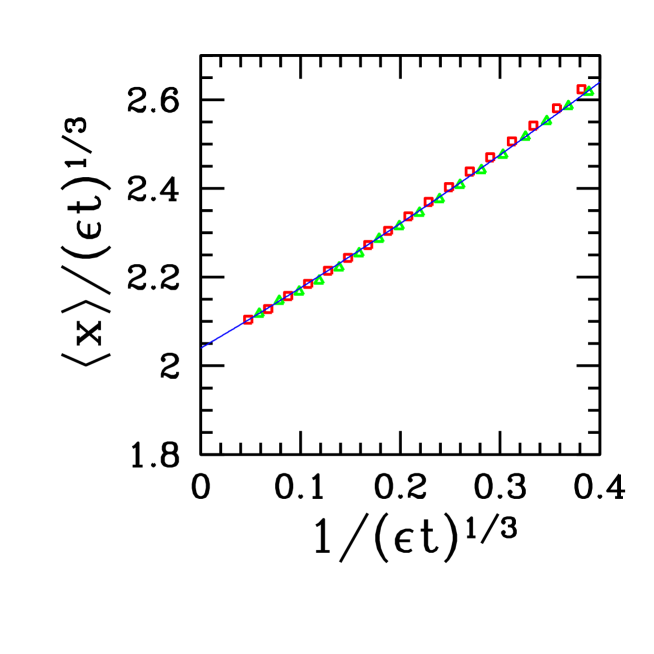
FIG. 3.: Scaled cluster size as a function of scaled time for the model with $\alpha=1$ and aggregated particle diffusion rates $\epsilon=0.001$ (squares) and $\epsilon=0.01$ (triangles). The solid curve is a parabolic fit of the data for $\epsilon=0.001$.

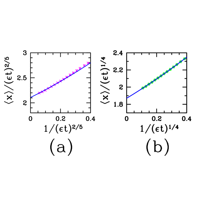
FIG. 4.: Scaled cluster size as a function of scaled time for the model with: (a) $\alpha=0.5$ and $\epsilon=0.001$; (b) $\alpha=2$ and $\epsilon=0.001$. The solid curves are parabolic fits of the data.

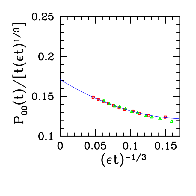
FIG. 5.: Scaled probability of double vacancies as a function of scaled time for the model with $\alpha=1$ and aggregated particle diffusion rates $\epsilon=0.001$ (squares) and $\epsilon=0.01$ (triangles). The solid curve is a parabolic fit of the data for $\epsilon=0.001$.

FIG. 6.: (a) Example of particle-hole configuration on a line and the map (dashed arrows) into a column problem. (b) The processes of particle detachment from clusters, with rate $\gamma$, and of free particle diffusion, with rate $1$, in the corresponding column picture. Filled squares are the particles whose diffusion rates were indicated.

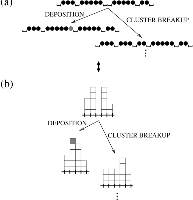
FIG. 7.: (a) Possible events after the formation of a double vacancy in the original particle picture: deposition of a new particle (grey circle) and one of the possible events of cluster breakup (left cluster) are illustrated. (b) The corresponding events in the column picture. Notice that deposition of a new particle (grey square) leads to the decrease of the lattice length in this picture.

FIG. 8.: Scaled probability of a cluster of size $m$ as a function of the scaled mass according to the prediction of the independent interval approximation (Eqs. 56 and 57), for: (a) $\alpha=2$, $\epsilon=0.001$, $z=1/4$, $t=4\times{10}^{7}$; (b) $\alpha=4$, $\epsilon=0.001$, $z=1/6$, $t=5\times{10}^{8}$.

FIG. 9.: Scaled probability of a cluster of size $m$ as a function of the scaled mass $y^{3/2}$, for: (a) $\alpha=0.5$, $\epsilon=0.001$, $z=0.4$, $t=4\times{10}^{6}$; (b) $\alpha=1$, $\epsilon=0.001$, $z=1/3$, $t=4\times{10}^{6}$.

FIG. 10.: Scaled probability of a cluster of size $m$ as a function of the scaled mass $y^{3/2}$, for: (a) $\alpha=2$, $\epsilon=0.001$, $z=1/4$, $t=4\times{10}^{7}$; (b) $\alpha=4$, $\epsilon=0.001$, $z=1/6$, $t=5\times{10}^{8}$.

- [1] R. B. Stinchcombe, Adv. Phys. 50, 431 (2001).
- [2] F. Ritort and P. Sollich, Adv. Phys. 52, 219 (2003).
- [3] M. R. Evans, J.Phys:Condens. Matter 14 1397 (2002).
- [4] D. Dhar, Physica A 315 5 (2002).
- [5] I. Koponen, M. Rusanen, and J. Heinonen, Phys. Rev. E 58, 4037 (1998).
- [6] F. D. A. Aarão Reis and R. B. Stinchcombe, Phys. Rev. E 70, 036109 (2004).
- [7] S. Clarke and D. D. Vvedensky, J. Appl. Phys. 63, 2272 (1988).
- [8] F. Family, P. Meakin, and J. M. Deutch, Phys. Rev. Lett. 57, 727 (1986).
- [9] P. Meakin and M. H. Ernst, Phys. Rev. Lett. 60, 2503 (1988).
- [10] F. Leyvraz and S. Redner, Phys. Rev. Lett. 88, 068301 (2002).
- [11] E. Ben-Naim and P. L. Krapivsky, Phys. Rev. E 68, 031104 (2003).
- [12] M. Bramson and J. L. Lebowitz, Phys. Rev. Lett. 61, 2397 (1988); 62, 694 (1989); J. Stat. Phys. 62, 297 (1991).
- [13] A. J. Bray and R. A. Blythe, Phys. Rev. Lett. 89, 150601 (2002).
- [14] R. A. Blythe and A. J. Bray, Phys. Rev. E 67, 041101 (2003).
- [15] Z. W. Lai, G. F. Mazenko, and O. T. Valls, Phys. Rev. B 37, 9481 (1988).
- [16] J. D. Shore, M. Holzer, and J. P. Sethna, Phys. Rev. B 46, 11376 (1992).