Quantum Statistics and Entanglement of Two Electromagnetic Field Modes Coupled via a Mesoscopic SQUID Ring.

Abstract

In this paper we investigate the behaviour of a fully quantum mechanical system consisting of a mesoscopic SQUID ring coupled to one or two electromagnetic field modes. We show that we can use a static magnetic flux threading the SQUID ring to control the transfer of energy, the entanglement and the statistical properties of the fields coupled to the ring. We also demonstrate that at, and around, certain values of static flux the effective coupling between the components of the system is large. The position of these regions in static flux is dependent on the energy level structure of the ring and the relative field mode frequencies, In these regions we find that the entanglement of states in the coupled system, and the energy transfer between its components, is strong.

I Introduction

In an earlier publication ClarkDREPPWS98 we considered the interaction of a quantum mechanical SQUID ring (a single Josephson weak link, capacitance $C_{s}$, enclosed by a thick superconducting ring, inductance $\Lambda_{s}$) with a classical electromagnetic (em) field. Using quasi-classical Floquet theory Hochstadt1986 ; shirley65 ; chu85 ; ho87 ; ChuJ91 ; cohen-tannoudji92:_atom_photon_inter to solve the time dependent Schrödinger equation (TDSE) for the SQUID ring, we were able to show that the ring-field interaction could be very highly non-perturbative in nature. In essence this is due to the ring Hamiltonian PranceCPSDR93 containing a cosine term (the Josephson coupling energy) which can generate non-linearities to all orders. In addition, this Hamiltonian and its solutions are $\Phi_{0}\left(=h/2e\right)$-periodic in the external static magnetic flux $\left(\Phi_{xstat}\right)$ applied to the ring. This quantum non-linearity ensures that energy exchange between the field and the ring is dominated by multiphoton absorption (and emission) processes ClarkDREPPWS98 . As we have demonstrated, this is the case even at modest field amplitudes and at frequencies much less than the separation between the ring energy levels $\left(\div h\right)$. In this work we showed that these energy exchanges occurred over very small regions in the bias flux $\Phi_{xstat}$. The values in $\Phi_{xstat}$ at which these exchanges take place are determined by the ring energy level structure and the field frequency $\left(\omega_{e}/2\pi\right)$ and flux amplitude $\left(\Phi_{e}\right)$. To be precise, it is in the exchange regions that the energy expectation value appears to jump (for example, using a two level model) between the time-averaged energies of the ground and first excited states of the ring. Each transition (exchange) region corresponds to the separation between the ring eigenenergies equalling $n\hbar\omega_{e}$, $n$ integer, leading to multiphoton absorption, or emission, between the ring and the field. It is in these regions that the non-linear nature of the ring Hamiltonian becomes manifest and where strong (and non-perturbative) time dependent superpositions occur between the original eigenstates of the ring.

Currently there is a great deal of interest in using mesoscopic SQUID rings (and other weak link based circuits) in quantum technologies, for example, in quantum computing Lopopescuspiller ; OrlandoMTvLLM99 ; MakhlinSS99 ; AverinNO90 . This interest has been stimulated by recent experimental work on probing quantum mechanical superposition states in Josephson weak link circuit systems RouseHL95 ; SilvestriniRGE00 ; NakamuraCT97 ; NakamuraPT99 , and even more so in the last year by reports of superposition states in SQUID rings FriedmanPCTL00 ; vanderWalWSHOLM00 ; Cosmelli2001 . It seems reasonable to assume that the theoretical description of weak link systems interacting with em fields (classical and quantum mechanical) is likely to be of great importance in the development of any future superconducting quantum technologies. In this regard the very strong non-linear behaviour exhibited by a single weak link SQUID ring in the exchange regions, referred to above, may prove to be of great utility. In order to test this viewpoint we have recently considered, within a fully quantum mechanical framework, the interaction of a SQUID ring with an oscillator field mode EverittSVVRPP2001 , i.e. the simplest coupled system we could have chosen (see figure 1).

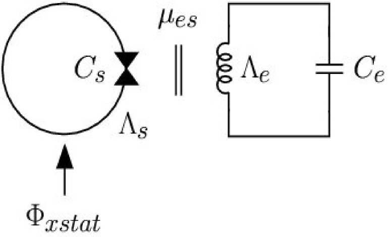
Figure 1: Block diagram of a SQUID ring coupled to a single em field mode of frequency $\omega_{e}\left(=1/\sqrt{C_{e}\Lambda_{e}}\right)$ where the flux linkage factor, ring to field mode, is $\mu_{es}$. Here, it is assumed that the temperature $T$ is such that $k_{B}T\ll\hbar\omega_{s},\hbar\omega_{e}$ for a SQUID oscillator frequency $\omega_{s}=1/\sqrt{C_{s}\Lambda_{s}}$ . Also shown is a static bias magnetic flux $\Phi_{xstat}$ applied to the ring.

We found that for the case of the em field in a coherent state the results derived from this quantum approach compare very well with those obtained previously using quasi-classical Floquet theory. In both approaches the ring and the field mode only couple strongly together within the exchange regions, i.e over certain narrow regions in the bias flux $\Phi_{xstat}$. This means that $\Phi_{xstat}$ can be used to control the coupling without losing superposition coherence in the system. We note that this work relates to quantum optical interactions in few level atoms and to few level systems involving either (superconducting) electron pairs or single electrons PranceCPSDR93 ; SchonZ90 ; MakhlinSS00 ; Kastner92 ; Grabert1992 .

These initial results for a two mode (ring + oscillator) system have encouraged us to draw more parallels with quantum optics. Rather than simply consider the SQUID ring as an electronic device, we may also view it as a tunable, $\Phi_{0}$-periodic, non-linear medium to couple a system of quantum oscillators together. Regarded as a non-linear medium, there is a clear analogy to other non-linear quantum systems in the context of quantum optics. However, there are two crucial differences, both of which may be of great importance in future quantum technologies. First, unlike the SQUID ring, in quantum optical systems the medium usually displays a weak polynomial non-linearity, even in strong fields WodkiewiczE85 ; YurkeMK86 ; CamposST89 ; FearnL89 ; singer1990 ; Vourdas92 . Second, all of the properties of the SQUID (quantum or quasi-classical) are $\Phi_{0}$-periodic in bias flux.

In this paper, our objective is to explore the consequences of the strong quantum non-linearity of the SQUID ring on the interaction, via the ring, of two oscillator field modes. This arrangement is depicted in figure 2,

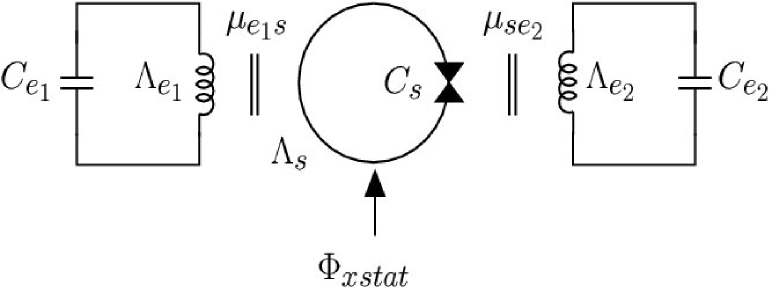
Figure 2: Block diagram of a SQUID ring coupled to two em field modes of frequency $\omega_{{e_{1}}}$ and $\omega_{{e_{2}}}$ assuming $k_{B}T\ll\hbar\omega_{s},\hbar\omega_{{e_{1}}},\hbar\omega_{{e_{2}}}$, with flux linkage factors $\mu_{e_{1}s}$ and $\mu_{se_{2}}$ between, respectively, the first field mode and the ring and the ring and the second field mode; all else as for figure 1.

with the two field modes and the ring oscillator frequencies taken to be $\omega_{{e_{1}}}/2\pi$, $\omega_{{e_{2}}}/2\pi$ and $\omega_{s}/2\pi=\frac{1}{2\pi\sqrt{\Lambda_{s}C_{s}}}$, respectively. As we shall see, the addition of the second field mode makes this a much more sophisticated and interesting system than the two mode system (ring+field oscillator) which was the subject of a recent publication EverittSVVRPP2001 , even though the computational demands that need to be met are very much greater. In this regard it is widely viewed Spillsuper ; OrlandoMTvLLM99 that the SQUID ring, as a coherent quantum device, has many potential applications in the design, development and operation of quantum mechanical circuits and quantum logic elements. In this paper we consider two aspects of the quantum behaviour of a SQUID ring which could have a serious impact in these areas, namely the transfer of entanglement and frequency conversion between em field modes via the quantum non-linearity of the ring. In this work we discuss frequency conversion and entanglement for just two field modes. However, if the non-linear aspects of quantum SQUID ring behaviour can be fully exploited more complicated operations could be envisaged. These may include using SQUID rings to couple/decouple entangled states in extended qubit circuit structures and allow frequency conversion processes between field modes to be modulated, producing coherent pulse modulated signals. In our opinion, the combination of such strong non-linear properties, coupled with $\Phi_{0}$-periodic external bias flux control of this behaviour, makes the SQUID ring quite unique as a device for application in quantum technologies. Thus, although the following calculations are concerned with some of the basic consequences of the quantum interaction of em field modes with a SQUID ring, we also wish to emphasize the technological possibilities which may open up as these ring-field mode systems become more fully understood.

In the work presented here we first consider briefly the two mode system, including a static bias flux $\Phi_{xstat}$ (figure 1). This allows us to relate the quasi-classical Floquet approach to the fully quantum mechanical treatment and demonstrate that our quantum model can produce consistent results. It also provides the background formalism for our main goal which is the study of two em field modes coupled through a SQUID ring. Since our purpose is to study the full quantum mechanics of the ring-field mode (1 or 2) system, we assume throughout that the operating temperature $\left(T\right)$ is such that $\hbar\omega_{{e_{1}},{e_{2}}}\gg k_{B}T$, $\hbar\omega_{s}\gg k_{B}T$. This ensures that both the ring and field mode(s) behave quantum mechanically. We then consider the extended quantum circuit, the two oscillator field modes ($\mathcal{E}_{1}$ and $\mathcal{E}_{2}$) coupled through a SQUID ring ($\mathcal{S}$) - figure 2 - with a bias flux $\Phi_{xstat}$ also coupled to the ring. In previous papers ClarkDREPPWS98 ; EverittSVVRPP2001 this bias flux was used to control the behaviour of the SQUID ring alone or the ring interacting with one field mode. In the current paper it is used to control the interaction between two field modes via the non-linear properties of the SQUID ring. At first sight there might appear to be no a priori reason why, in this three mode system, it should prove easy to couple all the components together strongly. However, at least for the case of weak inductive coupling between the modes, we shall show that well characterized energy exchange can take place at (or close to) certain specific values of $\Phi_{xstat}$. In these regions of bias flux multiphoton absorption and emission processes occur. Thus, the energy required for an interaction to take place is approximately equal to the energy transfer in the absorption or emission of an integer number of photons with frequency $\omega_{{e_{1}}}$ in the first field mode to an integer number of photons with frequency $\omega_{{e_{2}}}$ in the second. As for the two mode (ring+field mode) system, these are the exchange regions where the effective coupling becomes strong because of the non-linearity of the SQUID ring. As we shall see, it is in these regions that many interesting quantum phenomena can be observed.

To emphasize that the coupling across the extended three mode system is controlled by the bias flux, we calculate the average number of quanta in each mode and show that there is a large exchange of energy between the three modes at specific values of $\Phi_{xstat}$, thus demonstrating that frequency conversion can take place in the system. In addition, we also calculate the second order correlation $g_{i}^{(2)}$ (again controlled by the bias flux) which quantifies the quantum statistics (bunching of quanta) for all three modes ScullyZ97 . We show that as the system evolves in time, strong entanglement occurs between the three modes. We quantify this by calculating various entropic quantities based on the von Neumann entropy lindbland1973 ; lieb_bull1975 ; wehrl1978 ; BarnettP91 . These are chosen for convenience and familiarity and because they can be used to quantify the degree of entanglement between the subsystems (field modes and SQUID ring). Although these entropic quantities do have deficiencies as measures of entanglement Vedral1998 , there is no real consensus about which is the preferred measure within the quantum technology community. In the absence of any consensus, we opt for a familiar choice.

II The Two Mode Hamiltonian

II.1 The SQUID ring in a classical field

In our earlier work we treated the em field classically ClarkDREPPWS98 ; DigginsWCPPRS97-b and the SQUID ring quantum mechanically, using the well known Hamiltonian PranceCPSDR93

$$H_{s} = \frac{Q_{s}^{2}}{2C_{s}}+\frac{\left(\Phi_{s}-\left[\Phi_{xstat}+\Phi_{xem}\sin\omega_{e}t\right]\right)^{2}}{2\Lambda_{s}}$$ (1)

$$-\hbar\nu\cos\left(2\pi\frac{\Phi_{s}}{\Phi_{0}}\right)$$

Here, $\Phi_{s}$, the magnetic flux threading the ring, and $Q_{s}$, the electric displacement flux between the electrodes of the weak link in the ring, are the conjugate variables widom79 ; WidomC82-c for the system (with $\left[\Phi_{s},Q_{s}\right]=i\hbar$), $\hbar\nu/2$ is the matrix element for Josephson pair tunnelling through the weak link and $\Phi_{xem}$ is the amplitude of the classical magnetic flux at the ring due to the em field mode. With $\Phi_{xem}$ set to zero we can solve the time independent Schrödinger equation to find the eigenvalues of the SQUID ring alone as a function of applied flux $\Phi_{xstat}/\Phi_{0}$. As an example, we show in figure 3

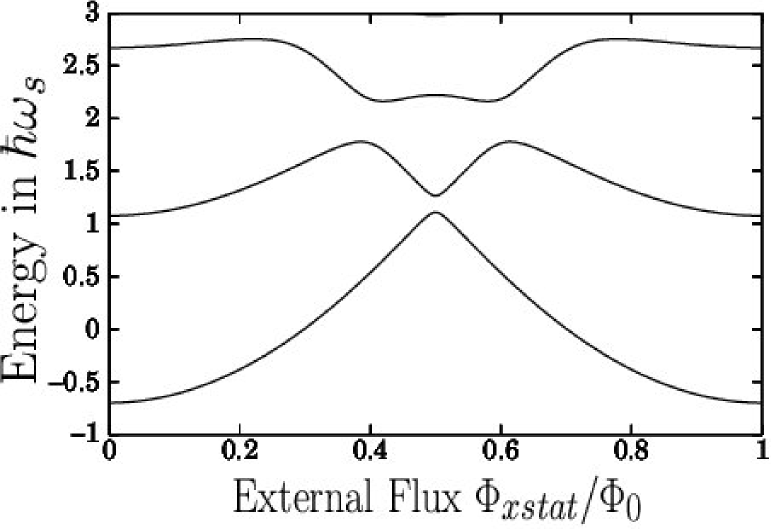
Figure 3: First three energy eigenvalues $E_{\kappa=0,1,2}$ of a quantum mechanical SQUID ring as a function of bias flux $\Phi_{xstat}/\Phi_{0}$ over the range $0\leq\Phi_{xstat}/\Phi_{0}\leq 1$ for $C_{s}=1\times 10^{-16}F$, $\Lambda_{s}=3\times 10^{-10}H$ $\left(\hbar\omega_{s}=0.043\Phi_{0}^{2}/\Lambda_{s}\right)$ and $\hbar\nu=0.07\Phi_{0}^{2}/\Lambda_{s}=1.63\hbar\omega_{s}\left(\nu=1.63\omega_{s}\right)$.

the first three eigenenergies of the ring [$E_{\kappa=0,1,2}\left(\Phi_{xstat}/\Phi_{0}\right)$, where $\kappa=0$ denotes the ground state, etc.] over the range $0\leq\Phi_{xstat}/\Phi_{0}\leq 1$ using parameters typical of a quantum regime SQUID ring ClarkDREPPWS98 ; EverittSVVRPP2001 , i.e. $C_{s}=1\times 10^{-16}$F, $\Lambda_{s}=3\times 10^{-10}$H (hence $\hbar\omega_{s}=0.043\Phi_{0}^{2}/\Lambda_{s}$ or $\frac{\omega_{s}}{2\pi}=9.8\times 10^{11}\mathrm{Hz}$) and $\hbar\nu=0.07\Phi_{0}^{2}/\Lambda_{s}=1.63\hbar\omega_{s}\left(\nu=1.63\omega_{s}\right)$. With $\Phi_{xem}$ turned on, we can use (1) to solve the corresponding TDSE. Again, by way of illustration, we show in figure 4

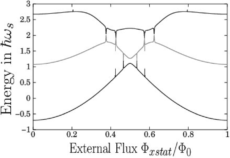
Figure 4: First three time averaged Floquet energies as a function of $\Phi_{xstat}/\Phi_{0}$ for the SQUID ring of figure 3 where, again, $\hbar\omega_{s}=0.043\Phi_{0}^{2}/\Lambda_{s}$ $\left(\frac{\omega_{s}}{2\pi}\approx 1\mathrm{THz}\right)$ and $\hbar\nu=0.07\Phi_{0}^{2}/\Lambda_{s}$ $\left(\nu=1.63\omega_{s}\right)$ with a classical em field of frequency$\omega_{xem}=0.5\omega_{s}$ and amplitude $\Phi_{xem}=2\times 10^{-3}\Phi_{0}$ applied. Here, the energy has been normalized to the ring oscillator energy $\hbar\omega_{s}$.

the computed time averaged ring energy expectation values for the first three Floquet states (eigenvalues of the evolution operator after one period of em field evolution) as a function of $\Phi_{xstat}/\Phi_{o}$ using the ring parameters of figure 3. Here, $\omega_{e}$ has been set at $0.5\omega_{s}$ with the associated $\Phi_{xem}=2\times 10^{-3}\Phi_{0}$. As can be seen, energy exchange between these time averaged energies occurs at specific values of the bias flux $\Phi_{xstat}$ and, as we have already pointed out, the number and position in $\Phi_{xstat}$ of these exchange regions depends on $\omega_{e}$, $\Phi_{xem}$ and the energy level structure of the ring. We have observed that these transition (exchange) points occur for values of bias flux such that (at least for small em field amplitudes $\Phi_{xem}$) $N\hbar\omega_{e}\approx E_{i}(\Phi_{x})-E_{j}(\Phi_{x})$ where $N=0,\pm 1,\pm 2,\ldots$ ClarkDREPPWS98 . We note that for the SQUID ring we can write down a renormalized oscillator frequency $\Omega_{s}=\omega_{s}+4\hbar^{2}\pi^{2}\nu\Phi_{0}^{-2}C_{s}^{-1}\omega_{s}^{-1}$ which is related to the fact that there is an $a_{s}^{\dagger}a_{s}$ term in a Taylor expansion of the cosine (Josephson) term in the ring Hamiltonian(1).

II.2 The SQUID ring in a non-classical field

In the fully quantum description the Hamiltonian $H_{t}$ for the SQUID ring-em oscillator mode system can be written as EverittSVVRPP2001

$$H_{t}=H_{e}+H_{s}-H_{es}.$$ (2)

where $H_{e}$ and $H_{s}$ are, respectively, the Hamiltonian contributions for the field and the ring and $H_{es}$ is the interaction energy linking these together.

Following equation (1), the Hamiltonian for the SQUID ring alone is PranceCPSDR93

$$H_{s}=\frac{Q_{s}^{2}}{2C_{s}}+\frac{\left(\Phi_{s}-\Phi_{xstat}\right)^{2}}{2\Lambda_{s}}-\hbar\nu\cos\left(2\pi\frac{\Phi_{s}}{\Phi_{0}}\right).$$ (3)

while the Hamiltonian for the em field (modelled as a parallel capacitance $\left(C_{e}\right)$ - inductance $\left(\Lambda_{e}\right)$ cavity mode equivalent circuit with infinite parallel resistance on resonance) takes the form $H_{e}=\frac{Q_{e}^{2}}{2C_{e}}+\frac{\Phi_{e}^{2}}{2\Lambda_{e}}$. Here, $\Phi_{e}$ and $Q_{e}$ are, respectively, the cavity mode magnetic flux and charge operators for a field mode frequency $\omega_{e}=1/\sqrt{C_{e}\Lambda_{e}}$. This cavity mode is coupled inductively to the SQUID ring with a coupling energy $H_{es}=\frac{\mu_{es}}{\Lambda_{s}}\left(\Phi_{s}-\Phi_{xstat}\right)\Phi_{e}$, where $\mu_{es}$ is the em field-SQUID ring flux linkage factor.

By making a suitable transformation [using the unitary translation operator ${\mathbb{T}=\exp\left(-i\Phi_{xstat}Q_{s}/\hbar\right)}$] the Hamiltonian (3) - now in calligraphic script - can be written more conveniently as

$$\mathcal{H}_{s}={\mathbb{T}^{\dagger}H_{s}\mathbb{T}=\frac{Q_{s}^{2}}{2C_{s}}+\frac{\Phi_{s}^{2}}{2\Lambda_{s}}-\hbar\nu\cos\left(2\pi\frac{\Phi_{s}+\Phi_{xstat}}{\Phi_{0}}\right)}$$ (4)

while the Hamiltonian for the em field mode remains unaffected. However, the interaction energy does transform to $\mathcal{H}_{es}=\frac{\mu_{es}}{\Lambda_{s}}\Phi_{s}\Phi_{e}$. We denote the magnetic flux dependent eigenstates of $\mathcal{H}_{s}$ by $|\sigma\rangle_{\mathcal{S}}$. In our computations we then use a truncated energy eigenbasis both for the ring ($\left|\sigma\right\rangle$)and the em field mode ($\left|n\right\rangle$). The basis states $\left|\sigma\right\rangle,\left|n\right\rangle$, where $\sigma=\alpha,\ldots,\Omega$ and $n=0,\ldots,N$, are taken so that $\Omega$ and $N$ are, respectively, much greater than the average number of quanta in the ring and em field.

Using this truncated basis, we can then solve

$$\mathcal{H}_{t}\left|\xi_{n}\right\rangle=\Xi_{n}\left|\xi_{n}\right\rangle$$ (5)

to obtain the eigenfunctions and eigenenergies of the two mode system Hamiltonian $\mathcal{H}_{t}$. The eigenenergies for the ring-field mode system are shown in figure 5

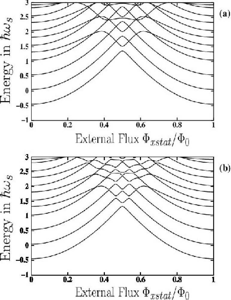
Figure 5: Eigenenergies of the SQUID ring-em field mode system (normalized in units of $\hbar\omega_{s}$) versus $\Phi_{xstat}/\Phi_{0}$ using the ring parameters of figure 3 with $C_{s}=C_{e}=1\times 10^{-16}F$, $\omega_{s}=2\omega_{e}$ $\left(\mathrm{where}\text{ }\frac{\omega_{s}}{2\pi}\approx 1THz\right)$ and $\nu=1.63\omega_{s}$. In (a) the field mode- SQUID ring flux linkage factor $\mu_{es}=0$; in (b) $\mu_{es}=0.1$.

for the $C_{s}$, $\Lambda_{s}$ and $\hbar\nu$ values used for figure 3, with $\omega_{s}=2\omega_{e}$, as in figure 4. Here, in figure 5(a) the field mode-ring linkage factor $\mu_{es}=0.0$ while in figure 5(b) it is $0.1$. From this spectral decomposition we can form the evolution operator via

$$U\left(t\right)=\sum_{n}\left|\xi_{n}\right\rangle\exp\left(-\frac{i\Xi_{n}t}{\hbar}\right)\left\langle\xi_{n}\right|$$ (6)

The time averaged energy expectation values $\langle\langle\mathcal{H}_{i=s,e}\rangle\rangle$ for the ring ClarkDREPPWS98 and the field (i.e. $\mathcal{H}{{{}_{s}}}$ and $\mathcal{H}_{{e}}$) can then be calculated using the expression

$$\langle\langle\mathcal{H}_{i}\rangle\rangle=\lim_{\tau\rightarrow\infty}\frac{1}{\tau}\int_{0}^{\tau}\mathrm{Tr}[\rho_{i}(t)\mathcal{H}_{i}]dt$$ (7)

where $\rho_{i},$ $i=e,s$ are the reduced density operators for the em mode and the SQUID ring, respectively. In practice, we have been able to ensure the convergence of the integral (7) by integrating numerically from $0$ up to $20,000/\omega_{s}$.

Clearly, provided we select the correct initial state for the em field in the two mode system, there should exist a correspondence between the Floquet method used in section II.1 [using (1)] and the result of a fully quantum mechanical calculation. As an initial state the coherent state is an obvious choice since it is the closest quantum state to a monochromatic em field, as used in the Floquet approach above. With this choice we would expect a reasonable agreement between the fully quantum and quasi-classical computations. In fact the match between these two approaches can be very good. To compare with the quasi-classical result of section II.1, we set the zero time $\left(t=0\right)$ product state as $|\alpha=i\sqrt{20}\rangle_{\mathcal{E}}\otimes|\sigma\rangle_{\mathcal{S}}$, where $|\alpha\rangle_{\mathcal{E}}$ is a coherent state of the field ($a_{e}|\alpha\rangle_{\mathcal{E}}=\alpha|\alpha\rangle_{\mathcal{E}}$ ). Using this coherent state we show in figure 6

Figure 6: Time averaged energy expectation values of $\mathcal{H}_{s}$ (in units of $\hbar\omega_{s}$) as a function of $\Phi_{xstat}/\Phi_{0}$ for comparison with figure 4 where the em-field mode is in a coherent state and the SQUID ring is in one of its first three energy eigenstates, i.e. the initial states are $|\alpha=i\sqrt{20}\rangle_{\mathcal{E}}\otimes|\sigma\rangle_{\mathcal{S}},$ $\left(\sigma=0,1,2\right)$. Here, as for figure 5, $C_{s}=C_{e}=1\times 10^{-16}F$, $\omega_{e}=0.5\omega_{s}\left(\mathrm{where}\text{ }\frac{\omega_{s}}{2\pi}\approx 1\mathrm{THz}\right)$, $\nu=1.63\omega_{s}$ but with $\mu_{es}=7.6\times 10^{-4}$ for comparison with figure 4.

the calculated $\left\langle\left\langle\mathcal{H}_{{s}}\right\rangle\right\rangle$ for an integration time $\tau=2\times 10^{4}/\omega_{s}$ with the energies normalized in units of $\hbar\omega_{s}$. The computations have been made over the range $0\leq\Phi_{xstat}/\Phi_{0}\leq 1$ for the values of $\sigma=0,1,2$, using the SQUID ring capacitance, inductance and $\Phi_{x}$-dependent energy level structure of figure 4 . Here, as for figure 3, we have made $\omega_{e}=0.5\omega_{s}$ while setting the flux linkage factor $\mu_{es}=0.00076$. We chose this value of $\mu_{es}$ so that the amplitude of oscillation of the coherent state in the em field coupled to the SQUID ring is equivalent to that used in the Floquet calculation of figure 4. It is apparent that the time averaged energy expectation values, and their exchange regions, calculated in the quantum model as a function of $\Phi_{xstat}$ are very close to those found using the quasi-classical Floquet approach. To emphasise this, we show in figure 7

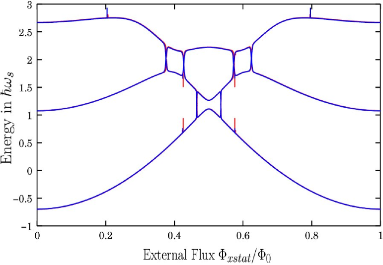
Figure 7: Comparison between time averaged energies of figures 4 (red) and 6 (blue).

the two calculations superimposed. The very close fit between the two gives us confidence that the quantum model is physically valid with an accurate correspondence to the quasi-classical regime when a coherent state is chosen for the em field.

As we have already noted for the SQUID ring in a classical field (section II.1), we observed that transition (or strong coupling) regions occur when $N\hbar\omega_{e}\approx E_{i}(\Phi_{x})-E_{j}(\Phi_{x}).$ From figure 5 we can see that this situation exists when degeneracies in the spectrum of the system are lifted due to the coupling term between the Hamiltonians for the SQUID ring and em field.

III The Three Mode Hamiltonian

Following on from (2), we now consider a SQUID ring with oscillator frequency $\omega_{s}$, threaded, as before, by a static bias flux $\Phi_{xstat}$, but now coupled to two em field modes of frequency $\omega_{{\ e_{1}}}$ and $\omega_{{e_{2}}}$ (see figure 2). With the usual flux $\left(\Phi_{i}\right)$-charge $\left(Q_{i}\right)$ commutation relation $\left[\Phi_{i},Q_{j}\right]=i\hbar\delta_{ij}$, the total Hamiltonian $\mathcal{H}_{\mathcal{T}}$ for this system can be written as

$$\mathcal{H}_{\mathcal{T}}=\mathcal{H}_{e_{1}}+\mathcal{H}_{e_{1}s}+\mathcal{H}_{s}+\mathcal{H}_{se_{2}}+\mathcal{H}_{e_{2}}.$$ (8)

where the SQUID ring Hamiltonian is given by (4) which has been transformed into the $\Phi_{xstat}$ basis. We choose to write our component Hamiltonians in (8) in terms of the annihilation $\left[a_{i}=\frac{1}{\sqrt{2}}\left(x_{i}+ip_{i}\right)\right]$ and creation $\left[a_{i}^{{\dagger}}=\frac{1}{\sqrt{2}}\left(x_{i}-ip_{i}\right)\right]$ operators as

$$\mathcal{H}_{e_{1}} =\hbar\omega_{{e_{1}}}\left(a_{{e_{1}}}^{{\dagger}}a_{{\ e_{1}}}+\frac{1}{2}\right)$$

$$\mathcal{H}_{e_{2}} =\hbar\omega_{{e_{2}}}\left(a_{{e_{2}}}^{{\dagger}}a_{{\ e_{2}}}+\frac{1}{2}\right)$$

$$\mathcal{H}_{s} =\hbar\omega_{s}\left(a_{s}^{{\dagger}}a_{s}+\frac{1}{2}\right)-$$

$$\hbar\nu\cos\left(\frac{2\pi}{\Phi_{o}}\sqrt{\frac{\hbar}{2C_{s}\omega_{s}}}\left(a_{s}^{{\dagger}}+a_{s}\right)+2\pi\frac{\Phi_{x}}{\Phi_{0}}\right)$$

where the position and momentum operators can be defined in terms of the magnetic flux and the charge operators via $x_{i}=\sqrt{C_{i}\omega_{i}/\hbar}\Phi_{i}$ and $p_{i}=\sqrt{1/C_{i}\hbar\omega_{i}}Q_{i}$ for oscillator frequencies $\omega_{i}=1/\sqrt{C_{i}\Lambda_{i}}$, with the subscript $i$ denoting ${e_{1}},{e_{2}}$ for the fields  or $s$ for the ring. Hence the Hamiltonians of the components of the system are identical (but extended to include an extra field mode) to those used in II.2, but written in terms of creation and annihilation operators.

The interaction energies $\mathcal{H}_{e_{1}s}$ and $\mathcal{H}_{se_{2}}$ in (8), each of which represents the inductive coupling between the SQUID ring and the oscillator modes ${e_{1}}$ and ${e_{2}}$, respectively, are given by

$$\mathcal{H}_{e_{1}s} =-\hbar\omega_{s}\frac{\mu_{e_{1}s}}{2}\sqrt{\frac{C_{s}\omega_{s}}{C_{{e_{1}}}\omega_{{e_{1}}}}}\left(a_{s}^{{\dagger}}+a_{s}\right)\left(a_{{e_{1}}}^{{\dagger}}+a_{{e_{1}}}\right)$$

$$\mathcal{H}_{se_{2}} =-\hbar\omega_{s}\frac{\mu_{se_{2}}}{2}\sqrt{\frac{C_{s}\omega_{s}}{C_{{e_{2}}}\omega_{{e_{2}}}}}\left(a_{s}^{{\dagger}}+a_{s}\right)\left(a_{{e_{2}}}^{{\dagger}}+a_{{e_{2}}}\right)$$

IV Time Evolution of the Three Mode System

The Hilbert space $\mathcal{T}$ for the SQUID ring-em field system is a tensor product of the Hilbert space $\mathcal{S}$ for the ring and the Hilbert spaces $\mathcal{E}_{1}$ and $\mathcal{E}_{2}$ for the fields, that is to say $\mathcal{T}=\mathcal{E}_{1}\otimes\mathcal{S}\otimes\mathcal{E}_{2}$. We denote in roman script the simple harmonic, em oscillator mode number eigenstates $|n\rangle_{i}$ ($a_{i}^{\dagger}a_{i}|n\rangle_{i}=n|n\rangle_{i}$). In representing the SQUID ring we use greek script, for example $|\alpha\rangle_{s},|\beta\rangle_{s},|\gamma\rangle_{s},\ldots,$ to represent the eigenstates of the Hamiltonian $\mathcal{H}_{s}$ in order to distinguish these from the number eigenstates $|n\rangle_{s}$ of the ring $\left(a_{s}^{\dagger}a_{s}|n\rangle_{s}=n|n\rangle_{s}\right)$.

In dealing with the time evolution of the coupled three mode system we must first solve the eigenproblem [see (5)] . As in section II for the two mode system, we use a truncated basis. This has the form

$$\big{\{} \left|N_{n,\kappa,m}\right\rangle\equiv\left|n\right\rangle_{{\mathcal{E}}_{1}}\otimes\left|\kappa\right\rangle_{\mathcal{S}}\otimes\left|m\right\rangle_{\mathcal{E}_{2}}|$$

$$n=0,...,N_{1},\,\kappa=\alpha,...,\Omega,\,m=0,...,N_{2}\big{\}}.$$ (9)

where $\left|n\right\rangle_{{\mathcal{E}}_{1}}$ and $\left|m\right\rangle_{\mathcal{E}_{2}}$ are the number states for the two field modes and $\left|\kappa\right\rangle_{\mathcal{S}}$ are the energy eigenstates of the SQUID ring Hamiltonian. Here, $N_{1}$, $\Omega$ and $N_{2}$ are taken to be much greater than the average number of quanta in each component of the system. With the eigenfunctions and eigenenergies of (5), but using the three mode Hamiltonian, the evolution operator can be calculated using the expression (6). Then, assuming that the system at $t=0$ is described by the density matrix $\rho(0)$, the density matrix $\rho(t)=U(t)\rho(0)U^{\dagger}(t)$ at a later time $t$ can be found, as can the reduced density matrices $\rho_{e_{1}}=\mathrm{Tr}_{{\mathcal{S}\otimes{\mathcal{E}_{2}}}}\left(\rho\right)$, $\rho_{s}=\mathrm{Tr}_{{{\mathcal{E}}_{1}}\otimes{\mathcal{E}_{2}}}\left(\rho\right)$, $\rho_{{e_{2}}}=\mathrm{Tr}_{{\mathcal{E}_{1}}\otimes\mathcal{S}}\left(\rho\right)$ and $\rho_{{e_{1}}s}=\mathrm{Tr}_{{\mathcal{E}_{2}}}\left(\rho\right)$, $\rho_{s{e_{2}}}=\mathrm{Tr}_{{\mathcal{E}_{1}}}\left(\rho\right)$, $\rho_{{e_{1}}{e_{2}}}=\mathrm{Tr}_{\mathcal{S}}\left(\rho\right)$. With these density matrices determined, we can then investigate a range of parameters which reveal much of the quantum behaviour of the three mode system, for example, the von Neumann entropy.

In the following sections of the paper we present numerical results demonstrating various aspects of this behaviour. Since the examples given are intended to be illustrative in nature, for simplicity we have made the capacitances for all three modes of the system the same, these being typical of quantum regime oscillators operating at a few K, i.e. $C_{{e_{1}}}=C_{{\ e_{2}}}=C_{s}=10^{-16}\mathrm{F}$. Amongst other things we wish to show that quantum frequency conversion can occur between the two oscillator field modes, via the SQUID ring. We have therefore made the two mode frequencies differ by a factor of two, i.e. $\omega_{{e_{1}}}=2\omega_{{e_{2}}}$ while again, for simplicity, setting $\omega_{{e_{1}}}=\omega_{s}$. With all capacitances identical these frequencies correspond to $\Lambda_{{e_{1}}}=\frac{1}{4}\Lambda_{{e_{2}}}=\Lambda_{s}$ for a typical SQUID ring inductance $\Lambda_{s}=3\times 10^{-10}\mathrm{H}$ (see section II). Again, as in section II, we have put $\hbar\nu=0.07\Phi_{0}^{2}/\Lambda_{s}\,\left(\nu=1.63\omega_{s}\right)$ which is typical value of the pair tunnelling matrix element for quantum regime SQUID rings operating at a few K. In addition, we have set the ring-field mode flux linkage factors at $\mu_{{e_{1}}s}=0.01$ and $\mu_{s{e_{2}}}=0.1$ which approximates to some reported experiments in the literature involving two oscillator field modes coupled through a SQUID ring WhitemanSCPPDR98 ; WhitemanCPPSRD98 .

IV.1 Strong Coupling of the SQUID ring to em field modes

In section II we demonstrated that strong coupling between the SQUID ring and the em field occurs when degeneracies in the spectrum of the Hamiltonian are lifted due to the coupling between the components of the system. Numerically, this equates to the condition $N\hbar\omega_{e}\approx E_{i}(\Phi_{x})-E_{j}(\Phi_{x})$, where $N$ is integer and the $E_{i}(\Phi_{x})$ and $E_{j}(\Phi_{x})$ are the $i^{th}$ and $j^{th}$ eigenvalues of the system Hamiltonian $\mathcal{H}_{t}$. These regions of strong coupling (the exchange regions), which develop at specific values of the bias flux $\left(\Phi_{xstat}\right)$ applied to the SQUID ring, are dependent on the ring eigenenergy structure and the frequency of the em field. Similarly, for the three mode system strong energy exchange will occur between the two field modes and the SQUID ring when the coupling terms lift degeneracies in the spectrum of the Hamiltonian. This will occur when

$$N_{{e_{1}}}\hbar\omega_{{e_{1}}}-N_{{e_{2}}}\hbar\omega_{{e_{2}}}\approx E_{i}(\Phi_{x})-E_{j}(\Phi_{x})$$ (10)

where, now, the $E_{i,j}(\Phi_{x})$ are the $i^{th}/j^{th}$ eigenvalues of $\mathcal{H}_{\mathcal{S}}$ and $N_{{e_{1}},{e_{2}}}$ are integers (positive or negative). In this case $N_{{e_{1}}}$ photons with frequency $\omega_{{e_{1}}}$ in the first field mode are used to excite the SQUID from the $j^{th}$-state to the $i^{th}$-state with the emission of $N_{{e_{2}}}$ photons of frequency $\omega_{{e_{2}}}$ into the second field mode. Taking the ring-field parameters set above, we have calculated the energy eigenvalues for the three mode system. These are shown in figure 8.

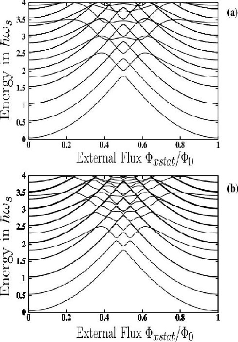
Figure 8: Eigenenergies (in units of $\hbar\omega_{s}$) versus $\Phi_{xstat}/\Phi_{0}$ of the three mode (em mode-ring-em mode) system with $C_{s}=C_{{e_{1}}}=C_{{e_{2}}}=1\times 10^{-16}F$, $\omega_{s}=\omega_{{\ e_{1}}}=2\omega_{{e_{2}}}\left(\mathrm{where}\text{ }\frac{\omega_{s}}{2\pi}\approx 1\mathrm{THz}\right)$, $\nu=1.63\omega_{s}$ and flux linkage factors $\mu_{e_{1}s}$ and $\mu_{se_{2}}$. In (a) $\mu_{e_{1}s}$ and $\mu_{se_{2}}$ are set equal to zero while in (b) $\mu_{e_{1}s}=0.01$ and $\mu_{se_{2}}=0.1$.

It can be seen that these eigenenergies possess a very rich structure which leads directly to the results presented in this paper.

Given a choice of the initial state for the fields in the two oscillator modes, we can calculate the time averaged energy expectation values (normalized in units of $\hbar\omega_{s}=\hbar/\sqrt{C_{s}\Lambda_{s}}$) of $\mathcal{H}_{{\ }e_{1}}$, $\mathcal{H}_{e_{2}}$ and $\mathcal{H}_{s}$ using equation (7) and integrating numerically from $0$ up to $2\times 10^{4}/\omega_{s}$. As an example, we show in figure 9(a)

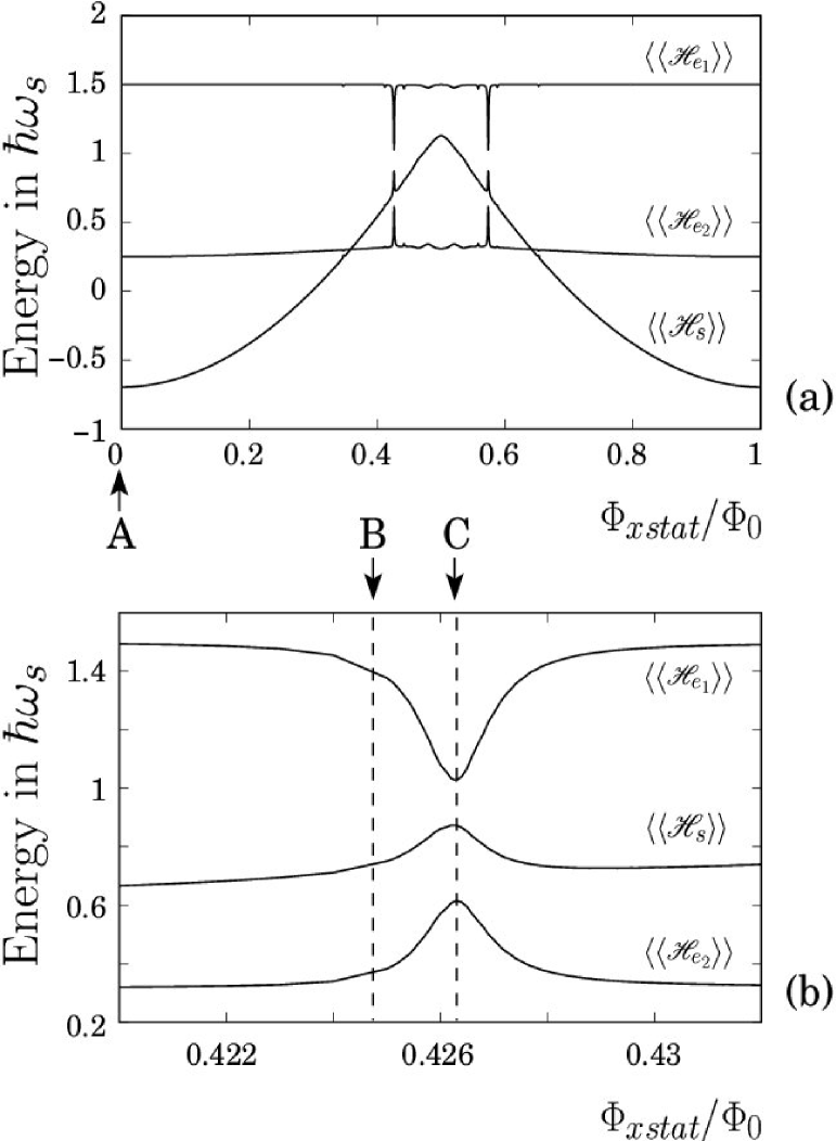
Figure 9: (a) Time averaged energy expectation values (in units of $\hbar\omega_{s}$) over the range $0\leq\Phi_{xstat}/\Phi_{0}\leq 1$ for the three mode system of figure 8 and (b) as for (a), but expanded around $\Phi_{xstat}/\Phi_{0}=0.426$. The initial state for the system is $\left|1\right\rangle_{\mathcal{E}_{1}}\otimes\left|\alpha\right\rangle_{\mathcal{S}}\otimes\left|0\right\rangle_{\mathcal{E}_{2}}$ and the circuit parameters are as in figure 8.

these time averaged energies plotted as a function of $\Phi_{xstat}/\Phi_{0}$ assuming that at $t=0$ the system is in the state $\left|1\right\rangle_{\mathcal{E}_{1}}\otimes\left|\alpha\right\rangle_{\mathcal{S}}\otimes\left|0\right\rangle_{\mathcal{E}_{2}}$, i.e. with one photon in the first em mode and none in the second. The peaks are a manifestation of the strong coupling between the various oscillators at and around specific values of $\Phi_{xstat}/\Phi_{0}$ where the energy transfer between the various components of the three mode system occurs. Thus, starting in the initial state $\left|1\right\rangle_{\mathcal{E}_{1}}\otimes\left|\alpha\right\rangle_{\mathcal{S}}\otimes\left|0\right\rangle_{\mathcal{E}_{2}}$, it can be seen that in the exchange regions, on average, energy is being transferred from the first mode to the SQUID ring and to the second mode. This will become more transparent when we compute the time evolution of the expectation values of the number operators for the components of the system (below). In figure 9(b) we show one of the three mode exchange regions (around $\Phi_{xstat}/\Phi_{0}=0.426$) of figure 9(a) on a much expanded scale so that the details can be seen more clearly.

IV.2 Quantum statistics of the SQUID ring-field system

An important aspect of non-classical electromagnetic fields is the quantum statistics of photons (bunching of photons) described by the second order correlations ScullyZ97 ; Bachor1998

$$g_{i}^{(2)}=\frac{\left\langle N_{i}^{2}\right\rangle-\left\langle N_{i}\right\rangle}{\left\langle N_{i}\right\rangle^{2}};\left\langle N_{i}^{M}\right\rangle=\mathrm{Tr}[\rho_{i}(a_{i}^{\dagger}a_{i})^{M}];i={\ e_{1}},{e_{2}},s$$ (11)

The value of $g^{\left(2\right)}=1$ corresponds to Poissonian statistics. Values of $g^{\left(2\right)}$ greater than 1 indicate photon bunching (i.e. where the photons arrive in groups) while values of $g^{\left(2\right)}$ smaller than one indicate antibunching (i.e. the regular arrival of photons). The latter regime is characteristic of non-classical electromagnetic fields since it can be shown that in classical optics $g^{\left(2\right)}\geq 1$. Only in quantum mechanical systems can $g^{\left(2\right)}<1$ ScullyZ97 ; Bachor1998 . This is well known in quantum optics but is, perhaps, less familiar in condensed matter physics.

In this work we show that the statistics of photons threading the SQUID ring affects the statistics of electron pair condensate tunnelling through the Josephson junction in the ring. This is quantified by the second order correlations although higher order correlations can also be calculated ScullyZ97 . These correlations fully describe the quantum statistics and quantum noise of the photons in the two field modes and the superconducting condensate.

IV.3 Quantum Entanglement in the Three Mode System

The creation of entangled states of multi-particle systems is a key feature of all quantum technologies. In their pursuit the generation of entanglements in real physical systems is clearly of very considerable interest. In this regard, it appears that the non-linear properties of the SQUID ring can be used very efficiently to entangle circuit subsystems (here, field oscillator modes) that are coupled to it. As we shall also show, the ring non-linearity can also be used with facility to generate energy conversion between the two oscillator field modes. Again, taking as our example the three mode system of figure 2, we shall demonstrate that as this system evolves in time its three components become, to a greater or lesser extent, entangled. The degree of this entanglement can be quantified by using entropic quantities. The entanglement for a two mode (ring-oscillator) system can be quantified by lindbland1973 ; lieb_bull1975 ; wehrl1978 ; BarnettP91

$$I_{AB}=S\left(\rho_{A}\right)+S\left(\rho_{B}\right)-S\left(\rho\right)$$ (12)

where $S\left(\rho\right)$ is the von Neumann entropy given by

$$S\left(\rho\right)=-\mathrm{Tr}\left[\rho\ln\left(\rho\right)\right]$$ (13)

with $\rho_{A}=\mathrm{Tr}_{B}\rho$ and $\rho_{B}=\mathrm{Tr}_{A}\rho$. This entanglement entropy is positive or zero (subadditivity property of the entropy). Examples of the calculation of this entanglement for the two mode system can be found in our previous work EverittSVVRPP2001 .

An analogous quantity can be used to characterize the entanglement of a three component system robinson67 ; Lanford68 ; Lieb73a ; Lieb73b . Thus, for the field mode-SQUID ring-field mode system, this takes the form

$$I=S\left(\rho_{{e_{1}}}\right)+S\left(\rho_{s}\right)+S\left(\rho_{{\ e_{2}}}\right)-S\left(\rho\right)$$ (14)

which can be written as

$$I=I_{{e_{1}}s}+I_{s{e_{2}}}+I\left({e_{1}}s;s{e_{2}}\right)$$ (15)

where $I_{{e_{1}}s}$ and $I_{s{e_{2}}}$ are the entanglement entropies between $\mathcal{E}_{1}\otimes\mathcal{S}$ and $\mathcal{S}\otimes\mathcal{E}_{2}$, as defined above (12), and

$$I({e_{1}}s;s{e_{2}})=S\left(\rho_{{e_{1}}s}\right)+S\left(\rho_{s{e_{2}}}\right)-S\left(\rho_{s}\right)-S\left(\rho\right)$$ (16)

describes a deeper entanglement between $\mathcal{E}_{1}\otimes\mathcal{S}$ and $\mathcal{S}\otimes\mathcal{E}_{2}$. Understanding of this deeper entanglement, that exists in three component systems, is intimately connected to the strong subadditivity property of the entropy. This can be used to demonstrate that the quantity $I(e_{1}s;se_{2})$ is positive or zero. We note that to prove this presented a very difficult problem in the theory of entropy (it was a conjecture for many years until a proof was provided robinson67 ; Lanford68 ; Lieb73a ; Lieb73b ).

In this paper we are not going to proceed further into this deep problem of entanglement in three component systems as it has been discussed in detail elsewhere Vourdas92 . However, we note that the entanglement $I$ can also be expressed as:

$$I =S\left(\rho_{{e_{1}}}\right)+S\left(\rho_{s}\right)+S\left(\rho_{{e_{2}}}\right)-S\left(\rho\right)$$ (17)

$$=I_{{e_{1}}s}+I_{{e_{1}}{e_{2}}}+I\left({e_{1}}s;{e_{1}}e_{2}\right)$$

$$=I_{{e_{2}}s}+I_{{e_{1}}{e_{2}}}+I\left(e_{2}s;{e_{1}}{e_{2}}\right)$$

where $I\left({e_{1}}s;{e_{1}}{e_{2}}\right)$ and $I\left({e_{2}}s;{e_{1}}{e_{2}}\right)$ are non-negative numbers. On physical grounds, i.e. because we are using the SQUID ring as the intermediary between the two field modes, we choose to show numerical results for the entanglement between the SQUID and the first mode ($I_{{e_{1}}s}$), the SQUID and the second mode ($I_{{e_{2}}s}$) and also the $I({e_{1}}s;s{e_{2}})$.

V Numerical Calculations

As we have shown in figures 6 and 9, strong coupling between the various of components of ring-field mode systems only occurs over small regions in $\Phi_{xstat}$ - the exchange regions. We now see how the variation in coupling across an exchange region affects the number operator expectation values, quantum statistics and entanglements - all important quantities reflecting on the quantum behaviour of these systems. Continuing from figure 9, we calculate these quantities at each of the three flux bias points A, B and C (at $\Phi_{xstat}/\Phi_{0}=0.0,0.4246$ and $0.4263$, respectively). In each of the following computed examples we assume that at $t=0$ the first field mode $\mathcal{E}_{1}$ contains one or more photons while the second contains none. In our first set of examples we choose the $t=0$ state in the first mode to be a number state; in the second set we make this a coherent state $|A\rangle_{\mathcal{E}{{}_{1}}}$, where $a_{{e_{1}}}|A\rangle_{\mathcal{E}{{}_{1}}}=A|A\rangle_{\mathcal{E}{{}_{1}}}$. For the case of the number state we assume that at $t=0$ the three mode system is in the state $|1\rangle_{\mathcal{E}{{}_{1}}}\otimes|\alpha\rangle_{\mathcal{S}}\otimes|0\rangle_{\mathcal{E}{{}_{2}}}$. For the example where we adopt a coherent state for the first mode we choose for illustrative purposes (and computational ease) the system state $|A=i\sqrt{3}\rangle_{\mathcal{E}{{}_{1}}}\otimes|\alpha\rangle_{\mathcal{S}}\otimes|0\rangle_{\mathcal{E}{{}_{2}}}$.

V.1 Number state computations

As is evident from figures 9(a) and 9(b), the flux bias points have been selected either to be well away from, or within, an exchange region, i.e. point A and points B and C, respectively. For a complete, quantitative view of the system we should compute, in sequence, the number expectation values $\left\langle n_{{e_{1}},s,{e_{2}}}\right\rangle$, the entropies $\left(I_{e_{1}s},I_{se_{2}},I\left({e_{1}}s;s{e_{2}}\right)\mathrm{\ and}\text{ }I\right)$and the $g_{{e_{1}},s,{e_{2}}}^{\left(2\right)}$ correlations for the first field mode $\left(\mathcal{E}_{1}\right)$, the SQUID ring $\left(\mathcal{S}\right)$ and the second field mode $\left(\mathcal{E}_{2}\right)$ as a function of normalized time $\omega_{s}t$. However, it is apparent in figure 10

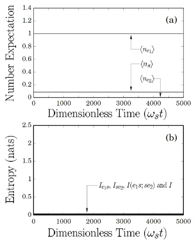
Figure 10: Starting in a pure state $|1\rangle_{\mathcal{E}_{1}}\otimes|\alpha\rangle_{\mathcal{S}}\otimes|0\rangle_{\mathcal{E}_{2}}$, plots of (a) the number expectation values $\left\langle n_{e_{1}}\right\rangle$, $\left\langle n_{s}\right\rangle$, $\left\langle n_{e_{2}}\right\rangle$ and (b) the entanglement entropies $I_{e_{1}s}$, $I_{se_{2}}$, $I\left(e_{1}s;se_{2}\right)$, $I$ versus dimensionless time $\omega_{s}t$ for the three component system of figure 9 with the ring flux biased at A in figure 9(a). Here, the system parameter values are as for figure 8(b).

(bias point A) that, starting in a pure state $|1\rangle_{\mathcal{E}{{}_{1}}}\otimes|\alpha\rangle_{\mathcal{S}}\otimes|0\rangle_{\mathcal{E}{{}_{2}}}$ for $\mathcal{E}_{1}$, the number expectation values (a) and entropies (b) remain constant as a function of time. We note that $\left\langle n_{s}\right\rangle$ is not zero because the ground state $\left|\alpha\right\rangle_{\mathcal{S}}$ of the SQUID ring is not the same as the ground state of a simple harmonic oscillator $\left|0\right\rangle$. From the definition given in section IV.2, the fact that $\left\langle n_{e_{2}}\right\rangle=0$ makes the calculation of $g^{\left(2\right)}$ for the second mode at bias point A physically unmeaningful since this is division by zero. It is therefore very sensitive to numerical error. However, such is not the case when the bias point point is shifted into an exchange region. Starting again with the system state $|1\rangle_{\mathcal{E}{{}_{1}}}\otimes|\alpha\rangle_{\mathcal{S}}\otimes|0\rangle_{\mathcal{E}{{}_{2}}}$, we show in figures 11

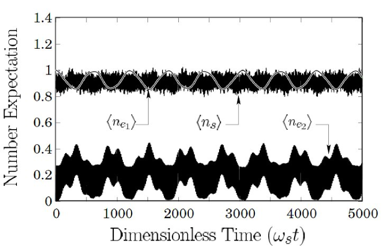
Figure 11: With the initial pure state $|1\rangle_{\mathcal{E}_{1}}\otimes|\alpha\rangle_{\mathcal{S}}\otimes|0\rangle_{\mathcal{E}_{2}}$, and with the parameter values of figure 8(b), a plot of the number expectation values $\left\langle n_{e_{1}}\right\rangle$, $\left\langle n_{s}\right\rangle$, $\left\langle n_{e_{2}}\right\rangle$ versus dimensionless time $\omega_{s}t$ for the static magnetic flux on the SQUID ring set at point B in figure 9(b).

(bias point B) and 12 (bias point C) the average number of quanta - the $\left\langle n_{i}\right\rangle$ - in each of the three modes as a function of time. With this choice of starting state these results demonstrate clearly the quasi-periodic exchange of energy between the various components of the system. Since the exchange coupling is strongest at C, this is where we would expect to find the maximum energy transfer between the first and second field modes, as is the case (figure 12).

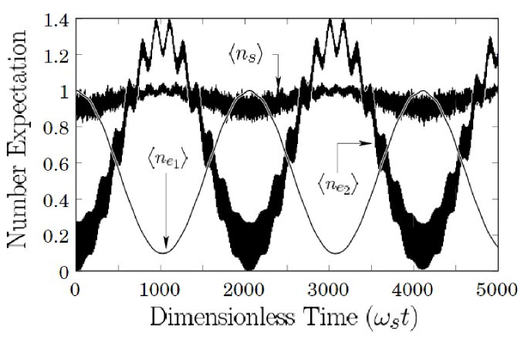
Figure 12: Starting in the pure state $|1\rangle_{\mathcal{E}_{1}}\otimes|\alpha\rangle_{\mathcal{S}}\otimes|0\rangle_{\mathcal{E}_{2}}$, and with the parameter values of figure 8(b), plots of the number expectation values $\left\langle n_{e_{1}}\right\rangle$, $\left\langle n_{s}\right\rangle$, $\left\langle n_{e_{2}}\right\rangle$ versus dimensionless time $\omega_{s}t$ for the three component system of figure 9 with the SQUID ring flux biased at point C in figure 9(b).

We note that in the computed results of figure 12 the second field mode number expectation value (and that of the SQUID ring to a much smaller extent) is a maximum when that for the first field mode is a minimum. This is the signature for frequency (down) conversion, in this example by a factor of two. The process could, of course, be run backwards to generate frequency up conversion from the second to the first field mode via the quantum non-linearity of the SQUID ring. Given that this non-linearity can be to all orders, we see no obvious reason why much higher ratio frequency conversions should not prove practicable.

From a theoretical viewpoint the problem with demonstrating high ratio frequency conversions is the rapid rise in the number of basis states required as the down (up) conversion frequency ratio increases. The computational difficulties increase accordingly. Nevertheless, even given the limitations on the computational power we have available (Compaq XP1000 alphaserver with 2GB RAM), we have been able to demonstrate quantum down conversion by a factor of ten in frequency. We intend to deal with this in a future publication. There is some indication that these down conversion processes occur WhitemanCPPSRD98 . In figure 12 the input state is the number state $|1\rangle_{\mathcal{E}_{1}}$ but, as we shall show, down conversion can occur for a coherent input state. It may well be that this ability to generate photon down/up conversion could have practical application for pure state sources in quantum information processing and quantum computing. For example, it may prove desirable to take single photon terahertz sources, as are now being developed FaistCSSHC94 ; amone2000 , and use these to provide the input state to a SQUID ring to generate photons at much lower frequencies suitable for solid state quantum circuit technologies. It is also clear that if very large down/up frequency conversion ratios can be achieved experimentally, there could well be interesting metrological applications, for example, in frequency standards.

This role in linking the two field modes together in a strongly non-linear, quantum mechanical manner is emphasized in figures 13

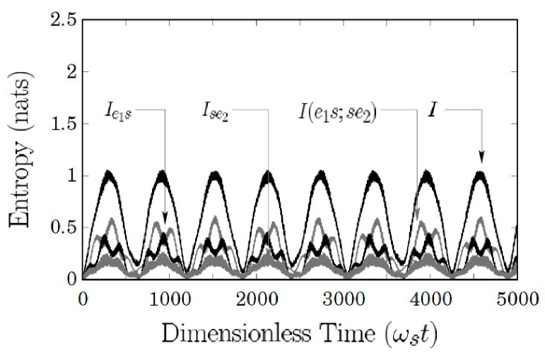
Figure 13: Entanglement entropies $I_{{e_{1}}s}$, $I_{s{e_{2}}}$, $I\left(e_{1}s;se_{2}\right)$ and $I$ versus dimensionless time $\omega_{s}t$ for the three component system of figure 9, with the parameter values of figure 8(b), starting in state $|1\rangle_{\mathcal{E}_{1}}\otimes|\alpha\rangle_{\mathcal{S}}\otimes|0\rangle_{\mathcal{E}_{2}}$ with the SQUID ring flux set at point B [figure 9(b)].

and 14

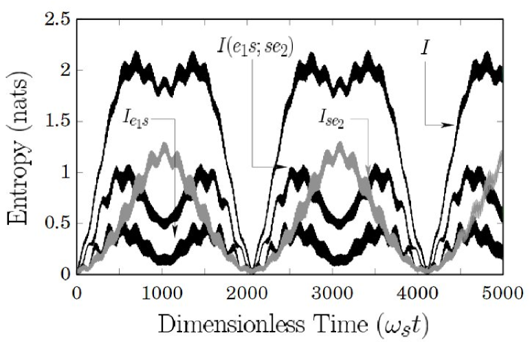
Figure 14: Entanglement entropies $I_{{e_{1}}s}$, $I_{s{e_{2}}}$, $I\left(e_{1}s;se_{2}\right)$ and $I$ versus dimensionless time $\omega_{s}t$ for the three component system of figure 9, with the parameter values of figure 8(b), starting in state $|1\rangle_{\mathcal{E}_{1}}\otimes|\alpha\rangle_{\mathcal{S}}\otimes|0\rangle_{\mathcal{E}_{2}}$ with the SQUID ring flux biased at point C in figure 9(b).

. Here, the time varying entanglement entropies are computed for bias points B (figure 13) and C (figure 14) following the definitions given in section IV.3. Here, again, we have started the system in state $|1\rangle_{\mathcal{E}{{}_{1}}}\otimes|\alpha\rangle_{\mathcal{S}}\otimes|0\rangle_{\mathcal{E}{{}_{2}}}$. It can be seen that the entanglement between the various components of the system ($I_{{e_{1}}s}$, $I_{s{e_{2}}}$ and $I\left({e_{1}}s;s{e_{2}}\right)$), and the total entanglement entropy for the system $\left(I\right)$, are stronger at C than at B which, from figures 9(b), 11 and 12, is to be expected. In our opinion it is this ability to control the degree of entanglement between the components of (for example) this three mode system simply by changing $\Phi_{xstat}$ which marks out the SQUID ring as a potentially very useful device in future quantum circuit technologies. This is emphasized by the contrast between figures 10(b) (for bias point A) and 14, where the system and subsystem entanglement go from zero to a maximum for an adjustment in $\Phi_{xstat}$ around $0.04\Phi_{0}$.

Although, in the above we have considered in some detail entanglement between two field modes (input and output) interacting via a SQUID ring, there are many other coupled systems of field modes and SQUID rings which could be studied. One which may be of importance, both scientifically and technologically, is an input field mode linked through a SQUID ring to two separate output modes at half the input frequency. From the results obtained in this paper we would expect the two (down converted) photons to be strongly entangled with the degree of entanglement controlled, again, by the bias flux $\Phi_{xstat}$ applied to the ring. Furthermore, given the non-linearity of the SQUID ring, we would also expect it to be possible to entangle a large number of output photons starting at an initial input frequency and down converting to a whole set of lower frequency output modes. As a technique, the use of a SQUID ring to generate entanglements between several systems could well be applied to great advantage in fundamental experimental studies of quantum mechanics Greenberger1990 ; Mermin1990 ; Macchiavello1999 . It could also have implications in quantum computing, for example, in creating an entangled input register for a quantum computer. It has also been suggested that the creation of (large number) multi-particle entangled systems could lead to new sensors and instrumentation of unparalleled sensitivity Brooks1999 and it may be that SQUID rings are very well suited to creating these entanglements, at least for photons.

There are other possible ways that the input register of a quantum computer could be based on the non-linear properties of SQUID rings described in this paper. For example, we could set the three modes of the coupled system in figure 2 all to have the same oscillator frequency $\omega_{s}$. Then, with $\Phi_{xstat}$ biased within an exchange region, we could arrange to create a qubit superposition state of $\left|0\right\rangle$ and $\left|1\right\rangle$ in the output mode starting from the number state $\left|1\right\rangle$ of the input mode. As our results have demonstrated, this could be done in such a way as to ensure that the input and output oscillator modes are entangled. Once the desired qubit state of the output mode had been realised, in principle the bias flux could then be switched away rapidly from the exchange region (or switched off) thus leaving the input and output modes entangled but uncoupled. An array of these circuits could then be used as an qubit register for a quantum computer, where the qubits would be entangled but not coupled to the input modes. Conceivably, this arrangement could facilitate quantum error correction for quantum computation Williamsclearwater1998 . Schemes of this kind may well find application in quantum encryption and transmission of information at a more complex level than is usually considered Lopopescuspiller ; Williamsclearwater1998 ; OpcitBrooks1999 .

Since the underlying purpose of this work is to demonstrate the influence of the SQUID ring non-linearity on a coupled quantum system, it is important to show quantitatively the way in which the quantum statistics of the photons affects the quantum statistics of the electron pairs (i.e. the superconducting condensate flowing through the weak link in the ring). As we explained above (section IV.2), this is quantified with the second order correlations $g_{i}^{\left(2\right)}$. In figures 15

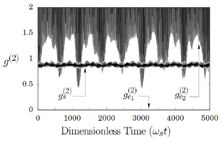
Figure 15: Second order correlations $g_{{e_{1}}}^{\left(2\right)},g_{s}^{\left(2\right)}$ and $g_{{e_{2}}}^{\left(2\right)}$ versus dimensionless $\omega_{s}t$ for the three component system of figure 9, starting in a pure state $|1\rangle_{\mathcal{E}_{1}}\otimes|\alpha\rangle_{\mathcal{S}}\otimes|0\rangle_{\mathcal{E}_{2}}$ with the static magnetic flux on the SQUID ring set at bias point B in figure 9(b). Here, the system parameter values are as for figure 8(b).

and 16

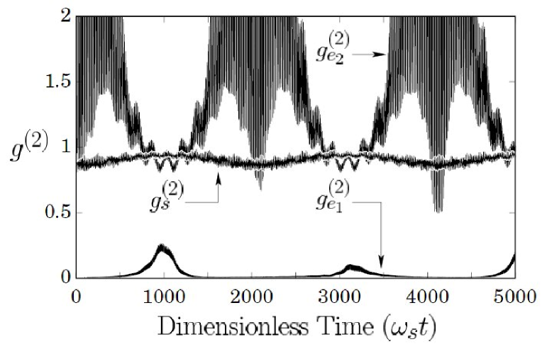
Figure 16: Second order correlations $g_{{e_{1}}}^{\left(2\right)},g_{s}^{\left(2\right)}$ and $g_{{e_{2}}}^{\left(2\right)}$ versus dimensionless $\omega_{s}t$ for the three component system of figure 9 [parameter values as for figure 8(b)], starting in a pure state $|1\rangle_{\mathcal{E}_{1}}\otimes|\alpha\rangle_{\mathcal{S}}\otimes|0\rangle_{\mathcal{E}_{2}}$ with the SQUID ring bias flux set at bias point C in figure 9(b).

we plot the second order correlations $g_{{e_{1}}}^{\left(2\right)}$, $g_{s}^{\left(2\right)}$ and $g_{{e_{2}}}^{\left(2\right)}$ for bias points B and C as functions of time with, again, a starting state for the system of $|1\rangle_{\mathcal{E}{{}_{1}}}\otimes|\alpha\rangle_{\mathcal{S}}\otimes|0\rangle_{\mathcal{E}{{}_{2}}}$. As with the number expectation values and the entanglement entropies, we see a strong oscillatory behaviour, particularly in figure 16 (biased at point C). In order to interpret the results we first note that for the state $|0\rangle_{i}$ $\left(i=\mathcal{E}{{}_{1}},\mathcal{E}{{}_{2}},\mathcal{S}\right)$, or other states close to this state, the average number of photons is near zero. From equation (11) this means that the second order correlation becomes very large. We also note for the number state $|1\rangle$, $\left\langle N^{2}\right\rangle-\left\langle N\right\rangle=0$ and the corresponding $g^{\left(2\right)}=0$. With this in mind, we see in figure 15 (bias point B) that the first field mode, in number state $|1\rangle_{\mathcal{E}{{}_{1}}}$ at $t=0$, starts with a $g^{\left(2\right)}$ at zero. It remains extremely close to this value over the time of the computation, i.e. this field mode stays reasonably close to the number state $|1\rangle_{\mathcal{E}{{}_{1}}}$. By contrast, the second field mode, assumed to be in the state $|0\rangle_{\mathcal{E}{{}_{2}}}$ at $t=0$, has on average a large $g^{\left(2\right)}$ value, although this dips well below unity almost periodically with time. This demonstrates that even at bias point B, on the edge of the exchange region, the value of $g_{e_{2}}^{\left(2\right)}$ regularly falls below one. It also shows that for this initial condition the quantum statistics of the second field mode cannot be described by classical means. In figure 16 (bias point C), at $t=0$, we again assume that the first field mode is in state $|1\rangle_{\mathcal{E}{{}_{1}}}$ with the second in state $|0\rangle_{\mathcal{E}{{}_{2}}}$. As before, the first field mode starts at $g_{{e_{1}}}^{\left(2\right)}=0$ but as the wavefunction for the system evolves with time we see that $g_{{e_{1}}}^{\left(2\right)}$ regularly shifts away from zero. Correspondingly, the first field mode is no longer in the pure number state $|1\rangle_{\mathcal{E}_{1}}$ due to its interaction with the rest of the system. The first field mode is described by a reduced density operator which, at these points, represents statistical mixture of states with a low photon number expectation value (as can be seen from figure 12). As a consequence, $g_{{e_{1}}}^{\left(2\right)}$ increases since the denominator in equation (11) becomes very small around these points.

V.2 Coherent state computations

In figures 17,

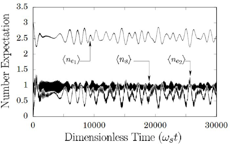
Figure 17: Starting the three component system with the first field mode in a coherent state, i.e. $|A=i\sqrt{3}\rangle_{\mathcal{E}_{1}}\otimes|\alpha\rangle_{\mathcal{S}}\otimes|0\rangle_{\mathcal{E}_{2}}$, and using the parameter values of figure 8(b), plots of the number expectation values $\left\langle n_{e_{1}}\right\rangle$, $\left\langle n_{s}\right\rangle$, $\left\langle n_{e_{2}}\right\rangle$ against dimensionless time $\omega_{s}t$ for the static flux on the SQUID ring set at point C in figure 9(b).

18

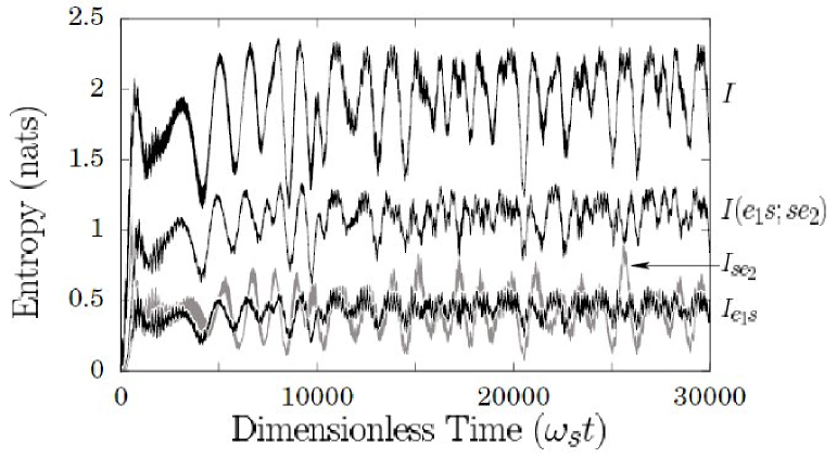
Figure 18: With initial state $|A=i\sqrt{3}\rangle_{\mathcal{E}_{1}}\otimes|\alpha\rangle_{\mathcal{S}}\otimes|0\rangle_{\mathcal{E}_{2}}$ for the three component system, the entanglement entropies $I_{{e_{1}}s}$, $I_{s{\ e_{2}}}$, $I\left(e_{1}s;se_{2}\right)$ and $I$ versus dimensionless time $\omega_{s}t$, where the system parameters are as for figure 8(b) and the SQUID ring is flux biased at point C in figure 9(b).

and 19

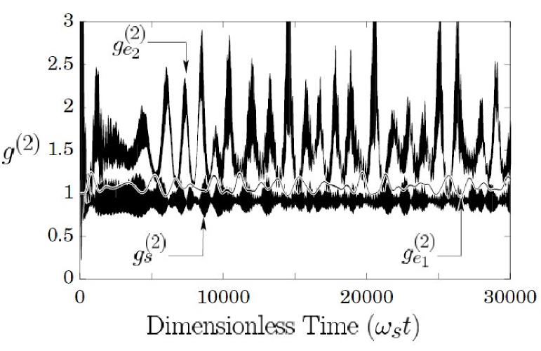
Figure 19: Second order correlations $g_{{e_{1}}}^{\left(2\right)},g_{s}^{\left(2\right)}$ and $g_{{e_{2}}}^{\left(2\right)}$ versus dimensionless time $\omega_{s}t$ for the three component system [parameter values as for figure 8(b)] starting in state $|A=i\sqrt{3}\rangle_{\mathcal{\ E}_{1}}\otimes|\alpha\rangle_{\mathcal{S}}\otimes|0\rangle_{\mathcal{E}_{2}}$ with the flux on the SQUID ring set at bias point C in figure 9(b).

we show the number expectation values, the entanglement entropies and the $g^{\left(2\right)}$ correlations for the bias point C in figure 9(b), taking the initial state of the system as $|A=i\sqrt{3}\rangle_{\mathcal{E}{{}_{1}}}\otimes|\alpha\rangle_{\mathcal{\ S}}\otimes|0\rangle_{\mathcal{E}{{}_{2}}}$, i.e. where the first field mode is in the coherent state $|i\sqrt{3}\rangle_{\mathcal{E}{{}_{1}}}$ at $t=0$ . It is apparent (figure 17) that there is energy transfer, via the SQUID ring, between the first and second field modes of the system, just as in figure 12 for the pure state $|1\rangle_{\mathcal{E}{{}_{1}}}\otimes|\alpha\rangle_{\mathcal{S}}\otimes|0\rangle_{\mathcal{E}{{}_{2}}}$ . Thus, when $\left\langle n_{{e_{1}}}\right\rangle$ decreases $\left\langle n_{{e_{2}}}\right\rangle$ increases, and vice versa. However, it is evident that the regular oscillatory behaviour seen in figures 11 and 12 has been lost. We note that, as in figures 11 and 12, the number expectation value of the SQUID ring remains at a roughly constant value, highlighting the view that the SQUID ring is acting as a non-linear control medium linking the two quantum field modes together. In figure 18 we see that the components of the system again entangled very strongly but, unlike the previous computations of figures 13 and 14, there is no longer any quasi-periodic disentanglement to be seen. The system remains entangled at all points in time, i.e. the total entanglement entropy is always high. In figure 19 there is clearly a significant deviation from the behaviour of the $g^{\left(2\right)}$ coefficients displayed in figures 15 and 16. Thus, in figure 19, $g_{{e_{1}}}^{\left(2\right)}$ is close to one for all of the time evolution (and for most of the time just greater than one) whereas $g_{s}^{\left(2\right)}$ spends most of its time just less than one and $g_{{e_{2}}}^{\left(2\right)}$ is almost always greater than one.

In all the examples given above we observe that, as expected, the system displays strong entanglement when the first field mode has a low number expectation value, i.e. the components of the system have evolved away from their initial pure states. We also note that when we start the first field mode in the pure state $|1\rangle_{\mathcal{E}{{}_{1}}}\otimes|\alpha\rangle_{\mathcal{S}}\otimes|0\rangle_{\mathcal{E}{{}_{2}}}$, at bias points B and C, we find strong entanglement between the various components of the coupled system which, at certain times (semi-periodically), disentangle. The entanglement entropies are, of course, theoretical quantities that demonstrate the development of quantum correlations between the three modes. In principle, experimental observation of these quantum correlations can be achieved by determining Bell type inequalities ScullyZ97 ; Bell1966 ; Williamsclearwater1998 . In the context of the work presented here this will require further theoretical investigation. In figures 15, 16 and 19 it is evident that the $g^{\left(2\right)}$ correlation coefficient for at least one of the components of the system becomes less than one at some point in the evolution of the system. Hence, for the initial conditions used in this work, we conclude that the photon statistics of this system cannot be described by classical optics.

VI Conclusions

In this paper we have studied the coupling of a SQUID ring to two em field modes. For this we have made the assumption that the ambient temperature of the system is low enough to be able to treat each of the three components (ring + two field modes) quantum mechanically. Our purpose has been to demonstrate that the SQUID ring, as a non-linear quantum object, can be used to couple a number of quantum oscillators together to generate physical phenomena of great interest. As we have emphasized, there exist obvious parallels with the field of quantum optics. However, in quantum optical systems the coupling media involved generally display only weak polynomial non-linearity. In contrast the SQUID ring, with the cosine term in its Hamiltonian description, can generate non-linear interactions to all orders. It is this, plus the $\Phi_{0}$-periodic nature of its behaviour as a function of external flux $\Phi_{x}$, which makes the SQUID ring of such interest in the burgeoning field of quantum circuit technology. Viewed from the perspective of quantum optics, the SQUID ring (or a set of coupled SQUID rings) can be thought of as a non-linear medium par excellence which can easily create very strongly coupled regimes (albeit at lower frequencies - for example, at THz frequencies and below) which are inaccessible using conventional optical materials.

In our theoretical investigations of the two em field modes coupled through a quantum SQUID ring we have also applied a static external magnetic flux $\left(\Phi_{xstat}\right)$ to the ring. In this paper we started with the simpler example of a SQUID ring interacting with a single em mode. We showed that the coupling between the components of the system can be strong. This strong coupling only occurs over small ranges in $\Phi_{xstat}$, centred around specific values of this bias flux, i.e. in what we term exchange regions which are govern by the energy eigenstructure of the system. It is in and around the exchange regions that the quantum non-linear nature of the SQUID ring is made manifest through the coupling of the field modes via the ring. For example, in these regions energy can be exchanged between the field modes and the SQUID ring and, through the intermediary of the ring, between the field modes themselves. From this we suggest that, suitably driven, this system may act as a frequency converter suitable for operation up to the THz range. From our viewpoint this illustrates the utility of these exchange regions since it is here that the strong quantum couplings develop between the components of the system. We have added to this perspective by calculating other physical phenomena associated with such a coupled quantum system. To illustrate this we have computed the statistics of the various quanta (quantified with the second order correlations) and the degree of entanglement (quantified with various entropies) between the components of the system, both outside and within the exchange regions. Our results demonstrate quite clearly that the mesoscopic SQUID ring can be used as a flux tunable element to manipulate these (and presumably other) quantum properties of these coupled circuit systems. As such, the work presented here may be of considerable relevance to current experiments on quantum superposition of states in SQUID rings and on probing crossing/anticrossing regions of their energy level structure FriedmanPCTL00 ; vanderWalWSHOLM00 ; Ralph2001 .

We note that we have neglected dissipation in the results presented in this paper. Thus, we have computed the time evolution of the three mode system using the equation $\partial_{t}\rho=-i[H,\rho]$. A more realistic calculation, with dissipation due to the environment taken into account (for example, in the references LeggettCDFGZ87, ; weiss1999, ; giulini1996, ) is now being developed. The equation for the time evolution then takes the form $\partial_{t}\rho=-i[H,\rho]+f(\rho)$, where a dissipative term $f(\rho)$ has been introduced to represent the environment. We intend to extend our work to investigate in detail the effects of this environmental dissipation on the behaviour of SQUID ring-field mode systems.

We suggest that the three component system (SQUID ring + two field modes), and its extensions, is rich in possibilities for device applications (e.g. in quantum gates, quantum encryption and frequency conversion); it is also a pointer to more sophisticated quantum technologies in the future Lopopescuspiller . Given that the technical problems associated with such technologies can be overcome, it seems likely that the SQUID ring (and related weak link circuits) will, in the future, be able to operate at THz frequencies. This could complement the current drive to develop THz applications in (classical) communications and imaging FaistCSSHC94 ; amone2000 . It would also allow for quantum circuit technologies to be utilized at quite accessible temperatures.

- (1) T. D. Clark, J. Diggins, J. F. Ralph, M. Everitt, R. J. Prance, H. Prance, R. Whiteman, A. Widom and Y. N. Srivastava, Annals Phys. 268, 1 (1998).
- (2) H. Hochstadt, The Functions of Mathematical Physics (Dover, New York, 1986).
- (3) J. H. Shirley, Physical Review 138(4B), 979 (1965).
- (4) S.I. Chu, Advances in Atomic and Molecular Phys. 21, 197 (1985).
- (5) T.S. Ho and S.I. Chu, Chem. Phys. Lett. 141, 315 (1987).
- (6) S. I. Chu and T. F. Jiang, Computer Phys. Comm. 63, 482 (1991).
- (7) C. Cohen-Tannoudji, J. Dupont-Roc, and G. Gynmerg, Atom-Photon Interactions (John Wiley, New York, 1992).
- (8) H. Prance, T. D. Clark, R. J. Prance, T. P. Spiller, J. Diggins, and J. F. Ralph, Nuclear Phys. B, pages 35–59, 1993.
- (9) H.K. Lo, S. Popescu, and T.P. Spiller, editors, Introduction to Quantum Computation and Information. (World Scientific, New Jersey, 1998).
- (10) T. P. Orlando, J. E. Mooij, L. Tian, C. H. van der Wal, L. S. Levitov, S. Lloyd, and J. J. Mazo, Phys. Rev. B-Condens Matter 60, 15398 (1999).
- (11) Y. Makhlin, G. Schon, and A. Shnirman, Nature 398, 305 (1999).
- (12) D. V. Averin, Y. V. Nazarov, and A. A. Odintsov, Physica B 165, 945 (1990).
- (13) R. Rouse, S. Y. Han, and J. E. Lukens, Phys. Rev. Lett. 75, 1614 (1995).
- (14) P. Silvestrini, B. B. Ruggiero, C. Granata, and E. Esposito, Phys. Lett. A 267, 45 (2000).
- (15) Y. Nakamura, C. D. Chen, and J. S. Tsai, Phys. Rev. Lett. 79, 2328 (1997).
- (16) Y. Nakamura, Y. A. Pashkin, and J. S. Tsai, Nature 398, 786 (1999).
- (17) J. R. Friedman, V. Patel, W. Chen, S. K. Tolpygo, and J. E. Lukens, Nature 406, 43 (2000).
- (18) C. H. van der Wal, A. C. J. ter Haar, F. K. Wilhelm, R. N. Schouten, C. J. P. M. Harmans, T. P. Orlando, S. Lloyd, and J. E. Mooij, Science 290, 773 (2000).
- (19) For coherence times see, for example, C. Cosmelli, P. Carelli, M.G. Castellano, F. Chiarello, G. Diambrini Palazzi, R. Leoni and G. Torriolo, Phys. Rev. Lett., 82, 5357 (1999); Siyuan Han, R. Rouse, Phys. Rev. Lett. 86, 4191 (2001); C. Cosmelli, Phys. Rev. Lett. 86, 4192 (2001).
- (20) M.J. Everitt, P. Stiffell, T.D. Clark, A. Vourdas, J.F. Ralph, H. Prance, and R.J. Prance, Phys. Rev. B 63, 144530 (2001).
- (21) G. Schon and A. D. Zaikin, Phys. Rep.-Rev. Sec. Phys. Lett. 198, 237 (1990).
- (22) Y. Makhlin, G. Schon, and A. Shnirman, Physica B 280, 410 (2000).
- (23) M. A. Kastner, Rev. Mod. Phys. 64, 849 (1992).
- (24) M.H.Devoret (Editors) H.Grabert, NATO ASI series, 294 (1992).
- (25) K. Wodkiewicz and J. H. Eberly, J. Opt. Soc. Am. B-Opt. Phys. 2, 458 (1985).
- (26) B. Yurke, S. L. McCall, and J. R. Klauder, Phys. Rev. A 33, 4033 (1986).
- (27) R. A. Campos, B. E. A. Saleh, and M. C. Teich, Phys. Rev. A 40, 1371 (1989).
- (28) H. Fearn and R. Loudon, J. Opt. Soc. Am. B-Opt. Phys. 6, 917 (1989).
- (29) F. Singer, R.A. Campos, M.C. Teich, and B.E.A. Saleh, Quant. Opt. 2, 307 (1990).
- (30) A. Vourdas, Phys. Rev. A 46, 442 (1992).
- (31) T.P. Spiller, “Superconducting Circuits for Quantum Computing”, Fortschritte Der Physik-Progress of Physics 48 (9-11):1075-1094 (2000).
- (32) M.O. Scully and M.S. Zubairy, Quantum Optics. (Cambridge University Press, 1997).
- (33) H-A. Bachor, A Guide to Experiments in Quantum Optics (Wiley-VCH, 1998).
- (34) G. Lindbland, Commun. Math. Phys. 33, 305 (1973).
- (35) E.H. Leib, Bull Am. Math. Soc. 81, 1 (1970).
- (36) A. Wehrl, Rev. Mod. Phys. 50, 221 (1978).
- (37) S. M. Barnett and S. J. D. Phoenix, Phys. Rev. A 44, 535 (1991).
- (38) See, for example, V. Vedral and M.B. Plenio, Phys. Rev. A 57, 1619 (1998).
- (39) J. Diggins, R. Whiteman, T. D. Clark, R. J. Prance, H. Prance, J. F. Ralph, A. Widom, and Y. N. Srivastava, Physica B 233, 8 (1997).
- (40) A Widom, J. Low Temp. Phys. 37, 449 (1979).
- (41) A. Widom and T. D. Clark, Phys. Letters A 90, 280 (1982).
- (42) R. Whiteman, V. Schollmann, T. D. Clark, R. J. Prance, H. Prance, J. Diggins, G. Buckling, and J. F. Ralph, J. Phys.-Condensed Matter 10, 9951 (1998).
- (43) R. Whiteman, T. D. Clark, R. J. Prance, H. Prance, V. Schollmann, J. F. Ralph, M. Everitt, and J. Diggins, J. Modern Optics 45, 1175 (1998).
- (44) J. Faist, F. Capasso, D. L. Sivco, C. Sirtori, A. L. Hutchinson, and A. Y. Cho, Science 264, 553 (1994).
- (45) D.D. Amone, C.M. Ciesla, and M. Pepper, Physics World 13(4), 35 (2000).
- (46) C.P. Williams and S.H. Clearwater, Explorations in Quantum Computing (Springer-Verlag, 1998).
- (47) M. Brooks (ed.), Quantum Computing and Applications (Springer-Verlag, 1999), p.46.
- (48) D.M. Greenberger, M.A. Horne, A. Shimony and A. Zeilinger, Am. J. Physics 58, 1131 (1990).
- (49) N.D. Mermin, Am. J. Physics 58, 731 (1990).
- (50) C. Macchiavello, G.M. Palma and A. Zeilinger (eds), Quantum Computation and Information Processing (World Scientific, 2000).
- (51) Op. Cit. reference 46, chapter 14..
- (52) W. Robinson and D. Ruelle, Comm. Math. Phys. 5, 288 (1967).
- (53) O. Lanford and D.W. Robinson, J. Math. Phys. 9, 1120 (1968).
- (54) E.H. Lieb and M.B. Ruskai, Phys. Rev. Lett. 30, 434 (1973).
- (55) E.H. Lieb and M.B. Ruskai, J. Math. Phys. 14, 1938 (1973).
- (56) J.S. Bell, Rev. Mod. Phys. 38, 447 (1966).
- (57) J.F. Ralph, T.D. Clark, M.J. Everitt, P. Stiffell, A. Vourdas, R.J. Prance and H. Prance, “The Behaviour of a Persistent Current Qubit in a Time Dependent Electromagnetic Field”, to be published in Proc. SPIE Conf., Quantum Computing II, Orlando, Florida, April 2001, SPIE Vol. 4386 Photonic and Quantum Technologies foe Aerospace Applications III, Eds. A.R. Pirich, E.W. Taylor and E. Donker (2001).
- (58) A. J. Leggett, S. Chakravarty, A. T. Dorsey, M. P. A. Fisher, A. Garg, and W. Zwerger, Rev. Mod. Phys. 59, 1 (1987).
- (59) U. Weiss, Quantum Dissipative Systems (World Scientific, Singapore 1999).
- (60) D. Giulini, E. Joos, C. Kiefer, J. Kupsch, I. -O. Stamatescu and H.D. Zeh, Decoherence and the Appearance of a Classical World in Quantum Theory (Springer-Verlag 1996).