Components of multifractality in high-frequency stock returns

Abstract

We analyzed multifractal properties of 5-minute stock returns from a period of over two years for 100 highly capitalized American companies. The two sources: fat-tailed probability distributions and nonlinear temporal correlations, vitally contribute to the observed multifractal dynamics of the returns. For majority of the companies the temporal correlations constitute a much more significant related factor, however.

The first, simple stock market model by Bachelier [1], based on Gaussian random walk, although it used to be applied for a long time, did not successfully pass practical tests as soon as large data samples were available and it was eventually rejected. The non-Gaussian distributions of price fluctuations, their persistent nonlinear temporal correlations, the intermittent behaviour present on all time scales and even the explicitly shown scaling invariance, together with some other properties of the stock market evolution, required introduction of more advanced and more appropriate models [2, 3, 4, 5, 6, 7]. What was especially interesting was the apparent similarity of the stock market dynamics to fluid turbulence [8], which led to the development of models based on the multiplicative cascades [9, 10, 11, 12, 13]. This sort of processes generate signals which are inherently multifractal with a continuous spectrum of scaling indices $f(\alpha)$ [14, 15]. Consistently, the real data from different financial markets (stock, forex and commodity ones) show clear multifractal properties [16, 17, 18, 19, 20, 21, 22, 23, 24].

It has already been pointed out in literature that the two fundamental factors leading to multifractal behaviour of signals are the nonlinear time correlations between present and past events and the fat-tailed probability distributions of fluctuations. Their role was analyzed both in models [25, 26] and in the real data from markets [23]. The latter work brought especially interesting results from a perspective of the present study: based on the stock and the commodity markets, authors of ref. [23] showed that, for the stocks, the main contribution to multifractality comes from a broad distribution of returns while a long memory present in this kind of data contributes only marginally. In opposite, for commodities the reported contribution of correlations is larger than for stocks. It should be noted that the nature of correlations leading to the multifractal dynamics of the returns is strongly nonlinear and, curiously, cannot be simply related to some well-known correlation type like a slowly decreasing volatility autocorrelation with an imposed daily pattern. For example, one even has to consider the nonlinear dependencies in the volatility itself in order to reveal how the temporal correlations contribute to multifractality in the stock market data.

A widely used method of quantifying multifractal properties of time series is the (multifractal) detrended fluctuation analysis (MF-DFA) [27]. For a time series of $N_{s}$ logarithmic returns $g_{s}(i)=\ln p_{s}(t_{i}+\Delta t)-\ln p_{s}(t_{i})$ of a stock $s$ (where $p_{s}(t_{i})$ stands for price at discrete time $t_{i}$), one calculates the signal profile

$$Y(i)=\sum_{k=1}^{i}{(g_{s}(k)-<g_{s}>)},\ i=1,...,N_{s}$$ (1)

where $<...>$ denotes averaging over the whole time series. Then $Y(i)$ is divided into $M_{s}$ disjoint segments of length $n$ ($n<N_{s}$) starting from both the beginning and the end of the time series so that finally one has $2M_{s}$ such segments. For each segment $\nu$, the local trend has to be calculated by fitting a $l$-th order polynomial $P_{\nu}^{(l)}$ to the data. In the next step one calculates the variance for all $\nu$’s and $n$’s

$$F^{2}(\nu,n)=\frac{1}{n}\sum_{j=1}^{n}\{Y[(\nu-1)n+j]-P_{\nu}^{(l)}(j)\}^{2}$$ (2)

and average it over $\nu$’s, obtaining the $q$th order fluctuation function

$$F_{q}(n)=\bigg{\{}\frac{1}{2M_{s}}\sum_{\nu=1}^{2M_{s}}[F^{2}(\nu,n)]^{q/2}\bigg{\}}^{1/q},\ \ q\in\mathbf{R}$$ (3)

for all choices of $n$. For a signal with fractal properties, the functional dependence $F_{q}(n)$ reveals power-law scaling

$$F_{q}(n)\sim n^{h(q)}$$ (4)

for sufficiently large $n$. The final product of the MF-DFA procedure is a family of scaling exponents $h(q)$ (generalized Hurst exponents) which for an actual multifractal signal form a decreasing function of $q$ (for monofractals $h(q)=const$). From the spectrum of generalized Hurst exponents one can calculate the singularity spectrum $f(\alpha)$ by using the following relations:

$$\alpha=h(q)+qh^{\prime}(q)\hskip 28.45274ptf(\alpha)=q[\alpha-h(q)]+1.$$ (5)

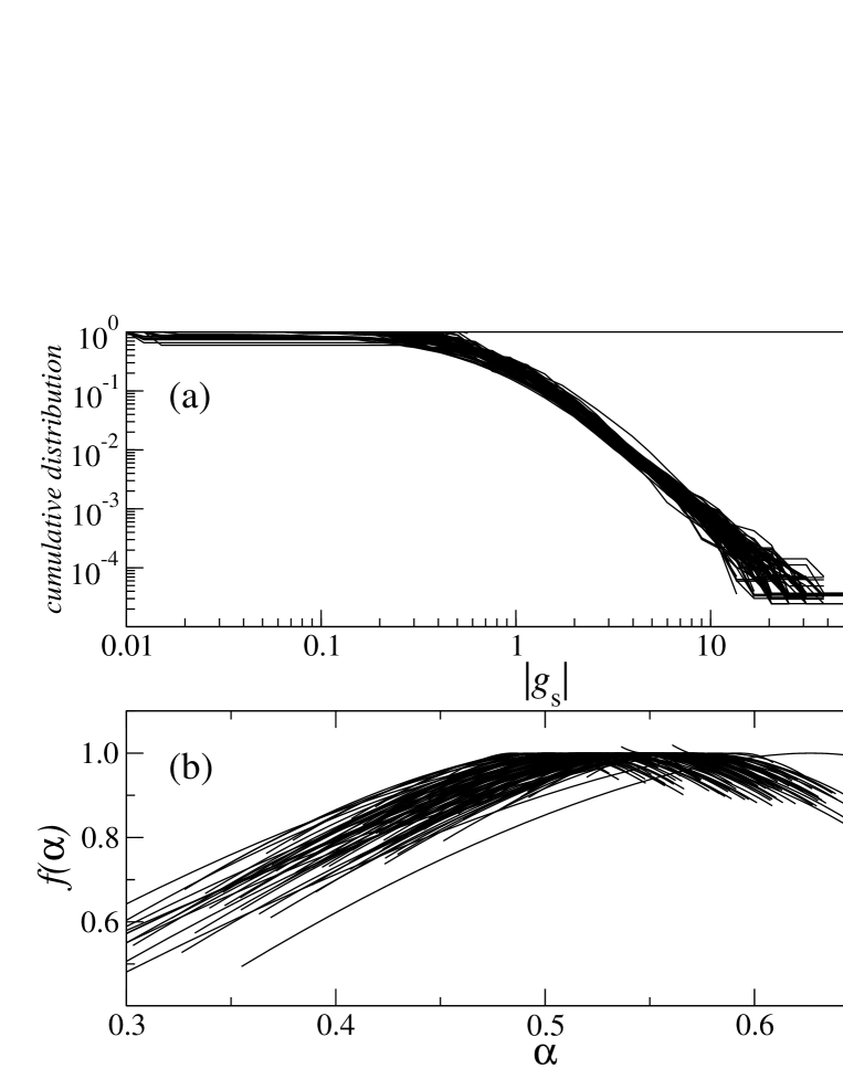
Figure 1: (a) The cumulative distribution functions of normalized stock returns for the 100 companies under study and (b) their singularity spectra $f(\alpha)$.

We analyzed time series of 5-minute stock returns for the 100 largest American companies according to their capitalization at the end of 1999. All the stocks were traded on NYSE or NASDAQ. The time interval covered by our data was from Dec 1, 1997 to Dec 31, 1999. We chose $\Delta t=5$ min because our time series of about 40,000 points were long enough to obtain statistically significant results and also length of the longest intervals of a constant stock price (i.e. zero returns), which affect the results of the MF-DFA procedure, was reasonably small and didn’t exceed 30 points. In order to eliminate a possible bias of the results due to the largest fluctuations, we restricted the range of $q$ in MF-DFA to the interval (-3,3); this restriction is also desired because of the inverse cubic power law which practically rules out the existence of moments higher than for $q=3$. The companies which we analyzed represented various market sectors, various trading frequencies (0.01-1 transactions/s), and capitalization spread of an order of magnitude ($10^{10}$-$10^{11}$$). However, we did not observe any qualitative dependencies of the relevant statistical and multifractal properties for different stocks on these quantities. Figure 1 presents the c.d.f. of the returns (a) and of the singularity spectra $f(\alpha)$ (b) for all 100 stocks under study. While widths of the $f(\alpha)$ spectra rather vary among the stocks, their c.d.f.’s all scale with exponent $\simeq-3$.

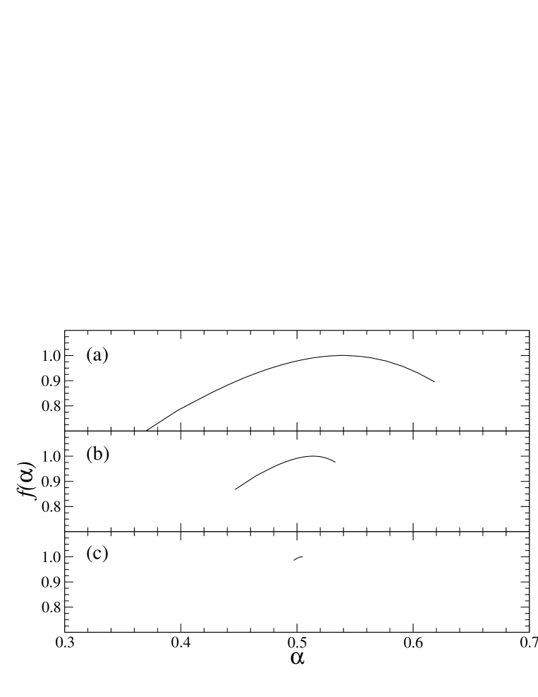
Figure 2: The singularity spectra $f(\alpha)$, calculated after averaging $h(q)$ over companies, for the original signals (a), for the reshuffled ones preserving distribution of the returns (b), and for the surrogates with both the distribution and the nonlinear correlations destroyed (c).

In order to separate the two possible sources of multifractality, i.e. the temporal correlations and the broad returns distributions, one can destroy the temporal structure of the signals by randomly reshuffling the corresponding time series of returns. What then remains are signals with exactly the same fluctuation distributions but without memory. Figure 2 shows the spectra $f(\alpha)$ averaged over all the companies for the original (a) and for the randomized (b) data. It is clear that these spectra are significantly different from each other, with the one for the randomized data being much narrower, i.e. much less multifractal than its counterpart for the real data. This indicates the important role of the temporal correlations as a source of multifractal dynamics of the stock returns. However, also the reshuffled data is of multifractal nature, which is in agreement with what the power-law behaviour of its distribution (Figure 1(a)) can suggest. A contribution to multifractality of the fat-tailed shape of the fluctuation distributions can be assessed by comparing the $f(\alpha)$ spectrum for the randomized data with the monofractal spectrum e.g. the one for the Fourier-phase-randomized surrogates. The surrogates are characterized by the same linear correlations (which do not produce multifractality [26]) as the original data but, by construction, for long signals their fluctuations are almost Gaussian. By comparing Figure 2(b) and Figure 2(c) one sees that in our case the fat-tailed distribution shape is also a meaningful source of multifractality, though rather weaker than the temporal correlations.

The contribution of correlations to the multifractal character of the high-frequency stock returns one can also quantify in another way, by considering variability of the generalized Hurst exponent $h(q)$ [28]. The idea is to compare the behaviour of $h(q)$ for the real and for the randomized data, while keeping in mind that an entire possible difference can be attributed to the influence of correlations. Let us define

$$h_{\rm corr}(q):=h(q)-h_{\rm rand}(q),$$ (6)

where $h_{\rm rand}(q)$ denotes $h(q)$ for the reshuffled signals. Since a multifractal signal is characterized by monotonously decreasing function $h(q)$ and since richer multifractality corresponds to stronger variability of $h(q)$, it is convenient to look at the quantity

$$\Delta h:=h(q_{\rm min})-h(q_{\rm max})$$ (7)

and its counterparts $\Delta h_{\rm rand}$ and $\Delta h_{\rm corr}$.

Contributions of the two sources to the multifractal spectra can be easily compared by computing the ratio $R=\Delta h_{\rm corr}/\Delta h_{\rm rand}$. The main panel of Figure 3 shows values of this ratio for all the companies under study. What can be clearly seen is that only a few stocks are characterized by $R\leq 1$ while most of the stocks fall within the range $1<R<5$. This result indicates that for the majority of stocks the temporal correlations are responsible for the most of the width of the multifractal spectra, leaving only the smaller remaining part for the distributions of returns. The plot also shows that the larger values of R are acompanied by the larger total width $\Delta h$. In fact, this behaviour is confirmed by the inset of Fig. 3, where $\Delta h_{\rm corr}(\Delta h)$ (full symbols) is firmly linear with slope $\sim 0.85$. $\Delta h_{\rm rand}(\Delta h)$ (open symbols) exhibits only a small positive slope $\sim 0.15$, suggesting that the multifractal component related to the distributions only weakly depends on $\Delta h$.

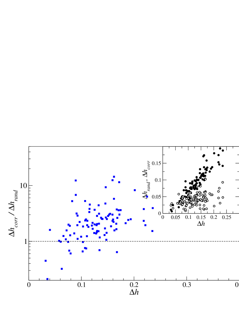
Figure 3: Main: multifractal spectra’s widths ratio $\Delta h_{\rm corr}/\Delta h_{\rm rand}$ versus $\Delta h$ for the individual companies. Inset: $\Delta h_{\rm corr}$ (full symbols) and $\Delta h_{\rm rand}$ (open symbols) vs. $\Delta h$. Weak dependence of the latter and strong linear relation of the former is visible.

Interestingly, the above observations apparently conflict with the results of ref. [23], where the dominating factor were the broad probability distributions of price fluctuations. However, by looking more carefully at the outcomes of both studies, it can be shown that they do not necessarily contradict each other. In fact, authors of ref. [23] analyzed daily returns, while we deal with the high frequency ones for which a nonlinear temporal structure is more complicated and more significant, with a more persistent memory (if time lag is measured in data points), with daily patterns and with intra-daily dependencies. It is not surprising also that in [23] it was the commodities which revealed a more meaningful correlation component than the stocks: due to the distinct nature of the commodities and the stocks, characteristic time scales for the former are much longer than for the latter and, thus, qualitatively, the price of the commodities sampled daily may well correspond to a more frequently sampled data for the stocks. Consistently, our results resemble the results for the commodities rather than for the stocks in [23].

One of the above-mentioned correlation types, the daily pattern of volatility, which is a well-known property of all trading markets, in itself is a subject worth bringing up in a context of the multifractal analysis. This pattern is sometimes considered as an uninteresting property of dynamics, thus often simply removed. Usually it is erased by dividing each return by standard deviation or average modulus of returns recorded at exactly the same moment of each trading day. Let us define a daily trend for a stock $s$ by square root of the expression

$$\sigma_{s}^{2}(k)=(1/n_{d})\sum_{j=1}^{n_{d}}(z_{s}^{(j)}(k)-<z_{s}^{(j)}(k)>_{j})^{2},$$ (8)

where $n_{d}$ denotes the number of returns in a trading day and the $k$th return of the $j$th trading day is denoted by $z_{s}^{(j)}(k)=g_{s}((j-1)*n_{d}+k)$. Then a detrended return $Z_{s}^{(j)}(k)$ reads

$$Z_{s}^{(j)}(k)=z_{s}^{(j)}(k)/\sigma_{s}(k).$$ (9)

This procedure e.g. leads to clearing the daily oscillations of the volatility autocorrelation. However, it should be noted that data without the intra-day volatility pattern present rather different statistical and dynamical properties than the original data. To illustrate this, we perform the multifractal analysis on the detrended (by standard deviation) data and compare results with the ones obtained for the non-detrended signals. First, the detrending alters probability distribution of the returns so that its tails are then thinner (Figure 4(a)) (see also [29]); in result, it is to affect the multifractal properties of such signals. Figure 4(b) shows the $f(\alpha)$ spectra for the original (solid) and the detrended (dashed) data; indeed, their distinct widths suggest that the multifractality of the latter is poorer than the one of the former. That this effect is in a large part due to the change of the probability distribution of the returns can be understood from Figure 4(c), in which the $f(\alpha)$ spectra for the reshuffled detrended signals (dashed) and the reshuffled original ones (solid) are presented. Here the difference between the spectra is associated with the corresponding difference between the distributions in Fig. 4(a). The spectrum for the detrended reshuffled signals, although rather narrow, is still of multifractal nature (it is significantly wider than its counterpart for signals derived from purely monofractal Gaussian noise, which resembles the spectrum in Fig. 2(c)). And what happens to that component of multifractality, which originates from correlations? For each individual stock, we calculated $\Delta h_{\rm corr}^{(d)}$ after the detrending and compared it to its non-detrended counterpart $\Delta h_{\rm corr}^{(n)}$ already displayed in Fig. 3. Outcome of this calculation can be viewed in Figure 5. Despite the fact that $\Delta h_{\rm corr}^{(n)}/\Delta h_{\rm corr}^{(d)}$ varies substantially from about 0.5 (detrending amplifies the component under discussion) up to 3 (detrending suppresses it), for a predominant group of stocks there is no visible change in $\Delta h_{\rm corr}$ (ratio $\simeq 1$). In the latter case the detrending does not modify those correlations which are responsible for the multifractal behaviour of signals, suggesting that for many stocks their so-removed intra-day volatility trend only marginally participates in multifractality.

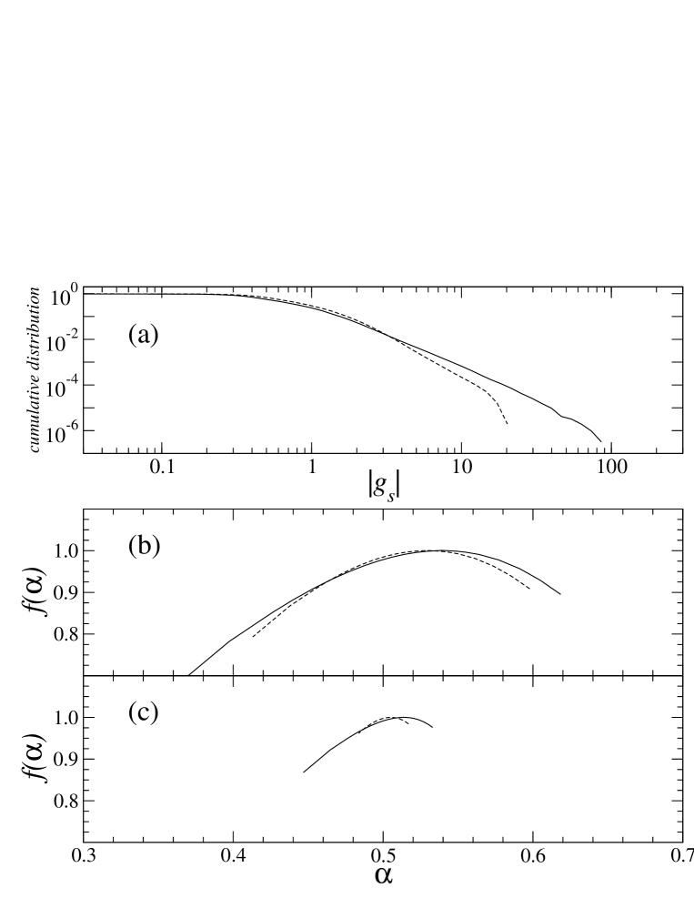
Figure 4: Comparison of statistical and multifractal characteristics of original (solid) and detrended (dashed) signals: cumulative probability distributions of returns (a), singularity spectra for actual data (b), and singularity spectra for reshuffled data (c). Each plot presents results averaged over 100 stocks.

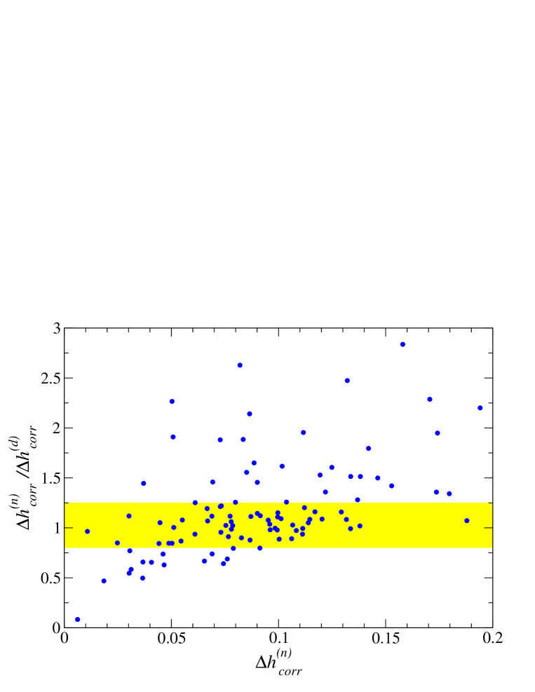
Figure 5: $\Delta h_{\rm corr}^{(n)}/\Delta h_{\rm corr}^{(d)}$ as a function of $\Delta h_{\rm corr}^{(n)}$; symbols represent individual companies; shaded region (0.80,1.25) comprises over 50% of stocks.

To summarize, we studied multifractal characteristics of the time series of 5-minute stock returns for the 100 largest American companies. Returns for all the stocks exhibit multiscaling, but their $f(\alpha)$ spectra have different widths. There are two fundamental sources of multifractality: the fat-tailed probability distributions of returns and the temporal correlations present in the data. The c.d.f. of returns are similar for all the stocks and, thus, their corresponding contribution to multiscaling is almost the same for each stock. In contrast, the temporal correlations are a factor whose influence is company-dependent and typically its strength is at least as large as the one for the return distributions. For the vast majority of stocks, the temporal correlations constitute a dominant factor spanning the spectrum. It is worthwhile to note that similar conclusions can be drawn from results presented in our previous paper [24] based on analysis of the German stocks. This convinces us that the above-described properties cannot be thought of as a unique attribute of the American stock market. Our results need to be confronted with earlier study from ref. [23] where, for daily stock returns, the multifractality was primarily related to the power-law probability distributions. The daily data, however, lacks to show so much temporal structure as the high-frequency returns do, and, in consequence, its multifractality is likely to reflect only this one source.

References

- [1] L. Bachelier, Ph.D. thesis, Sorbonne, Paris (1900)
- [2] B.B. Mandelbrot and J.W. van Ness, SIAM Review 10 (1968) 422-437
- [3] R.N. Mantegna and H.E. Stanley, Nature 376 (1995) 46-49
- [4] V. Plerou, P. Gopikrishnan, L.A.N. Amaral, M. Meyer and H.E. Stanley, Phys. Rev. E 60 (1999) 6519-6529
- [5] P. Gopikrishnan, V. Plerou, L.A.N. Amaral, M. Meyer and H.E. Stanley, Phys. Rev. E 60 (1999) 5305-5316
- [6] V. Plerou, P. Gopikrishnan, L.A.N. Amaral, X. Gabaix and H.E. Stanley, Phys. Rev. E 62 (2000) R3023-R3026
- [7] S. Drożdż, J. Kwapień, F. Gruemmer, F. Ruf and J. Speth, Acta Phys. Pol. B 34 (2003) 4293-4305
- [8] S. Ghasghaie, W. Breymann, J. Peinke, P. Talkner and Y. Dodge, Nature 381 (1996) 767-770
- [9] B.B. Mandelbrot, Fractal and Scaling in Finance: Discontinuity, Concentration, Risk, Springer Verlag (New York, 1997)
- [10] L. Calvet, A. Fisher, B.B. Mandelbrot, Large Deviations and the Distribution of Price Changes, Cowles Foundation Discussion Paper 1165 (1997)
- [11] T. Lux, The Multi-Fractal Model of Asset Returns: Its Estimation via GMM and Its Use for Volatility Forecasting, Univ. of Kiel, Working Paper (2003)
- [12] T. Lux, Detecting multi-fractal properties in asset returns: The failure of the ‘scaling estimator’, Univ. of Kiel, Working Paper (2003)
- [13] Z. Eisler and J. Kertész, Physica A 343 (2004) 603-622
- [14] T.C. Halsey, M.H. Jensen, L.P. Kadanoff, I. Procaccia and B.I. Shraiman, Phys. Rev. A 33 (1986) 1141-1151
- [15] A.-L. Barabási and T. Vicsek, Phys. Rev. A 44 (1991) 2730-2733
- [16] M. Pasquini and M. Serva, Economics Letters 65 (1999) 275-279
- [17] K. Ivanova and M. Ausloos, Physica A 265 (1999) 279-291
- [18] A. Bershadskii, Physica A 317 (2003) 591-596
- [19] T. Di Matteo, T. Aste and M.M. Dacorogna, cond-mat/0403681 (2004)
- [20] A. Fisher, L. Calvet and B. Mandelbrot, Multifractality of Deutschemark / US Dollar Exchange Rates, Cowles Foundation Discussion Paper 1166 (1997)
- [21] N. Vandewalle and M. Ausloos, Eur. Phys. J. B 4 (1998) 257-261
- [22] A. Bershadskii, Eur. Phys. J. B 11 (1999) 361-364
- [23] K. Matia, Y. Ashkenazy and H.E. Stanley, Europhys. Lett. 61 (2003) 422-428
- [24] P. Oświȩcimka, J. Kwapień and S. Drożdż, Physica A (in press), preprint cond-mat/0408277
- [25] H. Nakao, Phys. Lett. A 266 (2000) 282-289
- [26] T. Kalisky, Y. Ashkenazy and S. Havlin, cond-mat/0406310
- [27] C.-K. Peng, S.V. Buldyrev, S. Havlin, M. Simons, H.E. Stanley, A.L. Goldberger, Phys. Rev. E 49 (1994) 1685-1689
- [28] J.W. Kantelhardt, S.A. Zschiegner, E. Koscielny-Bunde, A. Bunde, S. Havlin and H.E. Stanley, Physica A 316 (2002) 87-114
- [29] B.H. Wang and P.M. Hui, Eur. Phys. J. B 20 (2001) 573-579