Record dynamics and the observed temperature plateau in the magnetic creep rate of type II superconductors.

Abstract

We use Monte Carlo simulations of a coarse-grained three dimensional model to demonstrate that the experimentally observed approximate temperature independence of the magnetic creep rate for a broad range of temperatures may be explained in terms of record dynamics, viz. the dynamical properties of the times at which a stochastic fluctuating signal establishes records.

I Introduction

The magnetization of type II superconductors is determined by the number of quantized magnetic vortices inside the sample [1]. As an externally imposed magnetic field is increased, vortices penetrate the sample in a process which at non-zero temperature is driven by thermal activation over energy barriers produced by the sample surface and by pinning centers in the bulk. When the external field is lowered, vortices leak out of the sample. The rate at which vortices move in and out of the sample determines the magnetic creep rate.

Given that the magnetic relaxation is driven by thermal activation, it is rather surprising that experiments have found the creep rate to be essentially temperature independent in a wide temperature range [2, 3, 4, 5, 6, 7, 8, 9, 10, 11, 12]. Several mechanisms have been suggested to explain how competing factors are able to cancel the typical Arrhenius temperature dependence $\exp(U/T)$ for activation over an energy barrier $U$. The most prominent theoretical suggestion so far is probably the description in terms of collective creep [13].

Here we show that the lack of temperature dependence of the creep rate can be understood quite simply in terms of record dynamics[14], which has recently been proposed as a general mechanism for the irreversible dynamics following a sudden quench in glassy systems [14, 15].

We base our analysis on the following two experimental and numerical observations:

• For a long time glitches have been observed in the time dependences of the magnetic relaxation of type II superconductors (see [12] and references therein). As the external magnetic field is varied, the magnetization undergoes abrupt jumps whenever vortices suddenly move in or out of the sample.

• A number of studies, experimental as well as theoretical [16, 17, 18, 19, 20, 21, 22, 23, 24, 25, 26, 27], indicates that in a broad range of not too high temperatures the vortex system exhibits many characteristic features of glassy dynamics.

Many [28, 29, 30, 31, 32, 33, 34, 35] but far from all [16, 17, 18, 19, 20] creep experiments study the response of the external magnetic field to a sweep, including sign reversal. For simplicity, we will presently concentrate on a setup in which the external field is initially ramped at a fixed rate up to a value and then remains constant for the entire duration of the experiment.

We use a three dimensional version of the Restricted Occupancy Model (ROM)[21, 22, 23, 24, 25, 26, 27] to study the response to a fixed applied magnetic field. Important physical properties of the 3D layered ROM model have a nearly temperature independent dynamical evolution, matching in this respect simulation results previously obtained for the same model [21, 22, 23, 24, 25, 26, 27] as well as experimental results on type II superconductors [3, 4, 5, 6, 11, 12, 16, 17, 18, 19, 20, 28, 29, 30, 31, 32, 33, 34, 35]. As a strong temperature sensitivity is expected for the activated dynamics of an entirely classical model system, the mechanism behind the observed temperature independence warrants some further theoretical scrutiny.

A fixed applied magnetic field can be expected to lead to a non-stationary time dependence of the internal magnetization which slowly increases from zero to about the value of the applied field. Interestingly, the low temperature dynamical evolution of the response involves two types of configuration rearrangements, having widely different time scales. One type consists of rapid glitches by which the magnetization irreversibly jumps to higher values, as additional vortices enter the system. We refer to these glitches as quakes [15, 36, 37] to emphasize their non-equilibrium nature, their abruptness and their dramatic effect on the state of the vortex system. The quakes are separated by much longer periods of apparent quiescence, during which the vortex system is ‘searching’ for a configuration of larger stability and for a way to accommodate more vortices inside the sample. Even though the total magnetization does not change, the internal spatial organization of the vortices undergoes considerable rearrangements.

We argue that the slow vortex creep associated with the quakes can be analyzed through the statistical properties of record dynamics, which immediately explains the temperature independence of the creep rate[14] for the range of temperatures for which this description is applicable. By record dynamics we mean the following. Consider a stochastic time signal $\chi(t)$. The corresponding record signal is $R(t)=\max_{\tau<t}\{\chi(\tau)\}$, i.e. the largest value assumed by $\chi(t)$ up to the current time $t$. The physical idea behind record dynamics [14, 36, 38, 39] is that large irreversible configurational changes in noisy systems with a macroscopic number of metastable attractors are induced by noise fluctuations of record size. Similar behavior is observed in other glassy metastable systems, e.g. gels and spin-glasses, and can be characterized statistically in a similar way [15, 36, 37]. This highlights the underlying unity of non-equilibrium glassy dynamics at low temperatures and supports the possibility of a common theoretical description.

The paper is organized as follows: The next Section summarizes the properties of the ROM model used in the simulations. Section III briefly introduces a possible mechanism [38, 39, 15] by which activated dynamics can become insensitive to the temperature in a glassy system, and demonstrates its relevance for the ROM model dynamics. Section IV focuses on creep rates and contains comparison with experiments. Finally, Section V presents a summary and a discussion.

II The 3D ROM model

The two dimensional Random Occupancy Model (ROM) has been shown to reproduce the essential features of vortex dynamics at nonzero temperature [21, 22, 23, 24, 25, 26, 27]. Here we use Monte Carlo (MC) simulations of a generalized three dimensional layered version of the ROM model to capture the long time relaxation of interacting vortex matter.

In vortex matter, the length scale of the interactions can be very large compared with the average distance between (pancake) vortices. At high densities, this implies that each vortex interacts with many others. For layered superconductors this situation can roughly be described by two length scales: the first is the range of the interaction parallel to the planes, this is the London penetration depth $\lambda$. The second length scale is the vortex correlation length, $\xi_{||}$, parallel to the applied field (which we imagine to be perpendicular to the copper oxide planes for high temperature superconductors). The exact identification of this length scale is difficult and is likely to depend on the anisotropy of the material, the nature of the pinning, the strength of the magnetic induction and on the temperature. This length scale may be related to vortex line cutting[40, 41, 42, 43, 44, 45, 46, 47]. These length scales respectively give the horizontal and vertical lattice spacing of our model. The horizontal coarse-grained length scale $l_{0}$, corresponds to the penetration depth $l_{0}=\lambda$ of the superconducting material, and the spacing between the layers in our lattice we consider $l_{1}\sim\xi_{||}$. Smaller length scales are ignored. For our purposes this approximation is acceptable because the length scales smaller than $\lambda$ seem to have little influence on the long time glassy properties of vortex matter.

Another limitation of the model is that it ignores the variation of $\lambda$ with the temperature. As will become clear from our ensuing discussion of record dynamics, ignoring the temperature dependence of $\lambda$ is not crucial for our explanation of the observed temperature plateau of the creep rate.

In a sample of a superconducting material the vortex matter behavior is determined by the competition of four energy scales [13]: intra and interlayer vortex-vortex interaction, vortex-pinning interaction and thermal fluctuations, all of which are schematically included in the ROM model.

The Hamiltonian of the ROM model is thus the following:

$$H=\sum_{ij}A_{ij}n_{i}n_{j}-\sum_{i}A_{ii}n_{i}+\sum_{i}A_{i}^{p}n_{i}+\sum_{\left\langle ij\right\rangle_{z}}A_{2}\left(n_{i}-n_{j}\right)^{2},$$ (1)

where $n_{i}$ is the number of vortices on site $i$ of the lattice. In a superconducting sample the number of vortex lines per unit area is restricted by the upper critical field ($B_{c2}$) [1], so in the model the number of vortices per cell can only assume values smaller than $N_{c2}=B_{c2}l_{0}^{2}/\phi_{0}$ [48, 25]. Hence the name Restricted Occupancy Model. Moreover, as we are interested in a simulation setup that does not require magnetic field inversion and the vortex-antivortex creation is strongly suppressed, we simply consider $n_{i}\geq 0$.

The first two terms in Eq. (1) represent the repulsion energy due to vortex-vortex interaction in the same layer, and the vortex self energy respectively. Since the potential that mediates this interaction decays exponentially at distances longer than our coarse-graining length $\lambda$, interactions beyond nearest neighbors are neglected. We set $A_{ii}:=A_{0}=1$, $A_{ij}:=A_{1}$ if $i$ and $j$ are nearest neighbors on the same layer, and $A_{ij}:=0$ otherwise.

The third term represents the interaction of the vortex pancakes with the pinning centers. $A_{i}^{p}$ is a random potential and for the purposes of this work we consider that $A_{i}^{p}$ has the following distribution $P\left(A_{i}^{p}\right)=\left(1-p\right)\delta\left(A_{i}^{p}\right)-p\delta\left(A_{i}^{p}-A_{0}^{p}\right)$. The pinning strength $\left|A_{0}^{p}\right|$ represents the total action of the pinning centers located on a site. In the present work we use $\left|A_{0}^{p}\right|=0.3$.

Finally the last term describes the interactions between the vortex sections in different layers. This term is a nearest neighbor quadratic interaction along the $z$ axis, so that the number of vortices in neighboring cells along the $z$ direction tends to be the same.

The parameters of the model are defined in units of $A_{0}$. The time is measured in units of full MC sweeps. The relationship between the model parameters and material parameters is discussed in [48, 25].

Each individual MC update involves the movement to a neighbor site of a single randomly selected vortex. The movement of the vortex is automatically accepted if the energy of the system decreases; if the energy of the system increases, the movement is accepted with probability $\exp(-\Delta E/T)$ [49].

Given that the movement of pancake vortices is restricted to the superconducting planes we only allow MC movements parallel to the planes. We have used periodic boundary conditions along the $z$ direction.

The external magnetic field is modeled by the edge sites on each of the planes. The density at the edge is kept at a controlled value. During a MC sweep vortices may move between the bulk sites and the edge sites. After each MC sweep the density on the edge sites is brought to the desired value. Initially the external field is increased to a desired value ($N_{ext}=10$ vortices per edge site) by a very rapid increase in the density on the edge sites. We have here used a sweeping rate $\gamma$ of 0.25 per MC sweep (compared with $\gamma\in[10^{-6},10^{-2}]$ in our previous studies [21, 22, 23, 24, 25, 26, 27]). After this fast initial ramping the external field is kept constant, while we study how the vortices move into the sample. The age of the system, $t_{w}$, is taken to be the time since the initial ramping.

We have studied systems of different sizes, and obtain similar results except for very small system sizes. Our key results were obtained in a system consisting of 8 layers of size $16\times 16$. The model parameters used in our simulations were:

number of realization $$=4000$$

$$A_{1} =0.28$$

$$A_{2} =0.5$$

$$p =0.5$$

$$A_{0}^{p} =0.3$$

$$N_{c2} =27$$

$$\gamma =0.25$$

$$N_{ext} =10$$

III Record dynamics

We will in this section describe how the observed plateau in the temperature dependence of the magnetic creep rate can be explained in the framework of record dynamics. Let us first mention the salient features of what we mean by record dynamics. Consider a stochastic signal $\chi(t)$ with no time correlations. Now derive the record signal $R(t)=\max_{\tau<t}\{\chi(\tau)\}$. We note that $R(t)$ is a monotonous piecewise constant function which only increases its value at discrete times $t_{k}$, whenever $\chi(t)$ manages to fluctuate to a value larger than any encountered previously. For our present purpose, the most important property of the statistics of the record times $t_{k}$ is that the probability that exactly $q$ records occur during the time interval $[t_{w},t_{w}+t]$ (where $t_{w}$ is the time since the initiation), is to a good approximation Poisson distributed on a logarithmic time scale [14, 36], i.e.,

$$p(q)={\langle q\rangle^{q}\over q!}\exp(-\langle q\rangle)$$ (2)

with average number of quake events proportional to logarithmic time

$$\langle q\rangle=\alpha\log(1+t/t_{w}).$$ (3)

Here $\alpha$ is the logarithmic rate of events. To get the gist of the mathematics behind Eq. (2) (for full detail see ref. [14]), we note that since the largest outcome, i.e. the record, of $t$ independent trials is equally likely to occur at any of the $t$ instances in the sequence, it occurs at the first attempt with probability $1/t$. Hence, the probability $p(1)$ of exactly one record in $t$ trials is $1/t$, independently of the distribution of the underlying signal $\chi(t)$. It is important to point out that the same also holds for the general expression for $p(q)$ in Eq. (2). The independence of $p(q)$ on the distribution of random numbers corresponds to the independence of $\chi(t)$ on the thermal noise and will translate directly into the temperature independence of the creep rate.

It has recently been shown [38, 39, 15] that in (glassy) systems having a large number of dynamically inequivalent attractors, temperature independence of suitably coarse-grained dynamical variables can arise from the peculiar way in which the attractors are selected as the system evolves from a typically rather unstable initial configuration through gradually more stable ones. A similar noise insensitivity of stochastic dynamics has been observed with other types of noise, e.g. in driven dynamical systems [14, 50] and in evolutionary dynamics[51, 15].

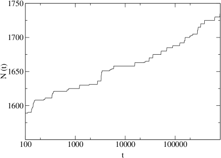
Figure 1: The detailed time variation of the total number of vortices $N(t)$ on the system for a single realization of the pinning potential and the thermal noise in a $8\times 8\times 8$ lattice for $T=0.1$. Notice the monotonous step function character of the time series.

That the ROM model also exemplifies this type of behavior can be gleaned from Fig. 1, showing the time dependence of the number of vortices $N(t)$ which during a single run have entered the system up to time $t$. Importantly, the length of the quiescent periods typically increases with time – notice the logarithmic time axis in Fig. 1. Were this not the case, the dynamics would appear continuous in terms of a suitably coarse-grained time scale. Conversely, the lengthening of the intervals between successive quakes signals the anticipated gradual entrenching of the dynamics into dynamically more stable configurations.

Also important is that the overwhelming majority of the observed glitches lead to states with a higher number of vortices. This de-facto irreversibility of the dynamics enables one to meaningfully approximate the signal $N(t)$ with the monotonically increasing record signal $R(t)=\max_{[0,t]}\{N(t)\}$. We stress that this theoretically convenient idealization is only applicable within the strongly non-equilibrium regime of our present concern.

Figure 2: (Color online) The main panel contains the temporal evolution of the probability density function, $P(N(t+t_{w})-N(t_{w}))$, of the number of vortices entering for $t_{w}=1000$ and three different observation times $t=188,2791,8371$ given by the black, slightly jagged, curves. The smooth curves (blue) are a fit to the theoretical expression (see Eq. (4)). The system is $16\times 16\times 8$ and $T=0.0001$. The insert shows the quake size distribution for various temperatures for the time interval between $t=1000$ and $t=10000$. For $T\leq 0.1$ the distribution has an approximately exponential tail. For $T=0.5$ the shape gets closer to a Gaussian.

Statistical insight into the time evolution in the number of vortices present within the system is provided by Fig. 2, where the empirical distributions of $N(t)$ are displayed for three different times, which are equidistantly placed on a logarithmic time axis. The insert in Fig. 2 shows the tail of the probability density function (pdf) of the number of vortices, $p(v)$, entering during a single quake. To a good approximation, the tail is exponential and the observed time dependence and temperature dependence of of $p(v)$ are negligible, except for the highest temperature $T=0.5$.

The interpretation in terms of record dynamics suggests that the probability that exactly $q$ quakes occur during the time interval $[t_{w},t_{w}+t]$ is Poisson distributed on a logarithmic time scale [14, 36] according to Eq. (2). We approximate the pdf for the number of vortices $v$ which enter during a given quake event (see insert Fig. 2) by an exponential distribution $p(v)=exp(-v/\bar{v})/\bar{v}$, and assume that subsequent quakes are statistically independent. The number of vortices entering during exactly $q$ quakes is then a sum of exponentially distributed independent variables, and is hence Gamma distributed. We finally obtain the pdf for the total number of vortices entering during $[t_{w},t_{w}+t]$ by averaging the Gamma distribution for $q$ quakes over the probability Eq. (2) that precisely $q$ quakes occur within the time interval of interest. This leads to the following expression for the pdf of total number of vortices $\Delta N=N(t+t_{w})-N(t_{w})$ which may have entered during the time interval $[t_{w},t_{w}+t]$

$$p(\Delta N,t)=e^{-{\Delta N\over\bar{v}}-\langle q\rangle}\sqrt{{\langle q\rangle\over\bar{v}\Delta N}}I_{1}\biggl{(}2\sqrt{{\langle q\rangle\Delta N\over\bar{v}}}\biggr{)},$$ (4)

where $I_{1}$ denotes the modified Bessel function of order $1$[52]. The above theoretical prediction, is compared in Fig. 2 with our simulation results. To estimate $\langle q\rangle$ according to Eq. (3), we used $\alpha=22.6$, as obtained from the logarithmic rate of the quake events. We can determine the average $\bar{v}$ in two ways. Either directly from the simulated distributions in the insert of Fig. 2 or from fitting Eq. (4) to the simulated data in the main frame of Fig. 2. In both cases we find $\bar{v}=16$. We also find that $\bar{v}$ is essentially temperature independent for temperatures below $T\approx 0.1$. This is also expected from the insert in Fig. 2. It is important to mention that the MC dynamics does overcome plenty of positive energy barriers, $\Delta E>0$, through thermal activation for temperatures in the range $0.01<T<0.1$. As the temperature is lowered fewer MC updates correspond to $\Delta E>0$ and for the lowest temperatures MC steps involve $\Delta E\leq 0$ only[24]. Nevertheless, the record dynamics remains essentially temperature independent for $T<0.1$.

The agreement is encouraging and suggests that the process of vortex penetration into the sample can be described in terms of a Poisson process with logarithmic time argument, for short the log-Poisson process. We also note that the log-Poisson statistics covers the temporal distribution of the quakes but has nothing to say on the size distribution of the jumps, i.e. the number $v$ of vortices entering during a single event. This stochastic quantity could in principle introduce additional time and temperature dependencies. However, as mentioned, the insert of Fig. 2 shows that for a very broad parameter range this is not the case. Accordingly, the creep rate obtained by convoluting the distribution of the quake sizes and the log-Poisson distribution of number of quakes will also be temperature independent.

The link between record statistics and the stochastic dynamics of a glassy system is discussed in detail in ref.[36] on the basis of several idealized physical assumptions. The first element is the existence of a large number, in principle a continuum, of attractors. These are sets of configurations clustered around a local energy minimum and supporting equilibrium-like reversible thermal fluctuations. By contrast, attractor changes—our quakes—are assumed to be irreversible on the time scale at which they occur. The exact nature of the quakes is not entirely clear in our system. At intermediate temperatures they are related to activation over barriers and the jump in $N(t)$ is associated with a increase in the energy of the interacting vortices. However, at the lowest temperatures there is not sufficient thermal energy available for the system to climb over energy barriers. The thermal fluctuations are only able to push the vortices along equipotential trajectories or to lower potential energy configurations. In this regime the vortex motion is hindered by jamming and the quakes are of a mechanical nature [24].

An interpretation in terms of record dynamics implies that the dynamical bottlenecks overcome by fluctuations are determined by the actual noise history, and not predetermined in a static fashion. For other model systems [14, 50], the validity of the assumed linkage between noise records and barriers was confirmed by considering white noise perturbations drawn from a distribution with finite support, e.g. a box distribution, and by then studying the properties of the selected attractors as a function of the maximum size of noise.

Record-induced dynamics has thus a number of testable predictions, the most interesting of which is, for our purposes, the logarithmic time dependence and the striking temperature independence of the number of quakes occurring in the time interval $[0,t]$, which are shown in the following Section.

IV
Creep rates

Let us now turn to the dependence on time and temperature of the total number of vortices in the sample. At time $t=0$ we rapidly increases the external field from zero up the value $N_{ext}$ (see section II). The vortex density of the bulk sites gradually increases as vortices move in from the boundary.

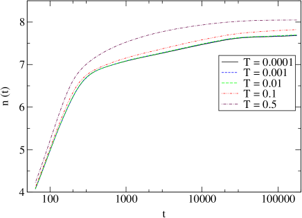
Figure 3: (Color online) Vortex density time dependence in the system for various temperatures. For $T\leq 0.1$ the vortex number is a piecewise linear function of $\log(t)$. For $T=0.5$ the system relaxation becomes faster. In this plot $n(t)$ is averaged over many system realizations.

In Figure 3 we present, for a very broad range of temperatures, the average density $n(t)$ of the bulk sites as function of the natural logarithm of time $\log(t)$. As anticipated, the time dependence is temperature independent for all but the highest temperatures.

One can identify three different temporal regimes separated at times $t_{1}\approx 300$ and $t_{2}\approx 3\times 10^{4}$. For the remaining of this paper we will focus our analysis on the intermediate regime $t_{1}<t<t_{2}$ (and choose $t_{w}=t_{1}$). Our reason for this is that at $t_{1}$ vortex interactions become essential through out the entire system. The late time regime $t>t_{2}$ is very difficult to resolve appropriately in simulations and probably equally difficult to study experimentally.

For times $t_{1}<t<t_{2}$ Fig. 3 demonstrates that $N(t)$ depends linearly on $log(t)$ to a very good approximation.

The linear logarithmic time dependence is of course entirely consistent with the record dynamics outlined in the previous section. We consider the total number of vortices in the system $N(t_{w}+t)$ to be the accumulated effect of vortices entering during quake events that have occurred prior to time $t_{w}+t$. Let $t_{k}$ denote the time of occurrence of quake number $k$ and let $v_{k}$ denote the actual number of vortices entering during this quake. We then have

$$N(t+t_{w})=N(t_{w})+\sum_{t_{w}<t_{k}<t_{w}+t}v_{k},$$ (5)

where the sum is over all quakes that occured during the time interval $[t_{w},t_{w}+t]$

From Fig. 2 we know that $v_{k}$ is temperature independent and possesses a well defined average $\bar{v}$. Since the average number of quakes increases according to Eq. (3), record dynamics predicts the following (temperature independent) temporal evolution of the average number of vortices

$$\Delta N\equiv\langle N(t+t_{w})\rangle-\langle N(t_{w})\rangle=\alpha\bar{v}\log(1+t/t_{w}).$$ (6)

i.e. for the considered time regime $t/t_{w}\gg 1$ a temperature independent logarithmic rate given by

$$d\Delta N/d\log(t)=\alpha\bar{v}/(1+t_{w}/t)\approx\alpha\bar{v}.$$ (7)

We extract the rate of the quakes in the simulations from temporal signals like the one exhibited in Fig. 1. In Fig. 4 we demonstrate that the quake rate is indeed approximately independent of temperature in the broad temperature interval $10^{-4}<T<2\times 10^{-2}$.

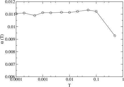
Figure 4: Quake dynamics rate, $\alpha$, versus $T$ for the time interval between $t=1000$ and $t=10000$. Notice that $\alpha$ is roughly temperature independent for three orders of magnitude below $T<0.1$.

Figure 5: (Color online) Main panel: Numerical results for the creep rate versus $T$ for the time interval between $t=1000$ and $t=10000$. In the low temperature region the creep rate is constant within our numerical precision for about two orders of magnitude - we observe a nonzero creep rate in the $T\rightarrow 0$ limit. Insets: experimental results for the creep rate versus T. The right inset shows data from Keller et al. for melt processed YBCO crystals with the magnetic field applied along the $c$ axis (squares) and $ab$ plane (circles). The left inset shows data from [53] for unirradiated (squares) and 3 MeV proton-irradiated (circles) YBCO flux grown [54] crystals with a 1 T magnetic Field applied parallel to the $c$ axis.

Finally, Fig. 5 shows the near temperature independence of the actual rate with which $N(t)$ changes. We extract this rate from the data shown in Fig. 3 in the time region $t_{1}<t<t_{2}$ and plot the normalized creep rate $S=d\log[M(t)]/d\log(t)$ in order to compare consistently with experiments, here we have used $M(t)=|N(t)-N_{ext}|$.

V Conclusion

We have presented an analysis of simulated vortex creep data in terms of record dynamics. This approach allows us to interpret the observed temperature independence of the creep rate as a generic property of the dynamics of records obtained from the underlying fluctuating sequence. To establish the temperature independence of the creep rate we do not need to know the detailed nature of the quantity being gradually maximized. Nor do we need a description of the intermittent vortex quakes which are responsible for the abrupt changes in the number of vortices. All we make use of is the assumption, supported by the simulated model, that the abrupt glitches in the number of vortices inside the sample can be interpreted as arising from the records of some stochastic process. We showed that the simulated creep rate behaves in a way very similar to published experimental data for YBCO.

It is obvious that a better experimental and theoretical understanding of the nature of the vortex quakes is interesting and future study of the ROM model will seek to improve our understanding of the spatial and dynamical properties of these quakes. We can already conclude that the physical mechanisms involved must be different at low and high temperatures. At the lowest temperatures activation over free energy barriers are excluded and the quakes are related to mechanical rearrangements of the vortices[24]. At elevated temperatures the quakes are expected to be triggered by activation over thermal barriers. The present paper shows that record dynamics can be used to understand the temperature range from very low temperatures, where no barriers can be climbed, up through a regime where thermal activation does take place. For high temperatures (in our case for $T>0.1$) the description in terms of record dynamics breaks down. This happens when there is sufficient thermal energy available to make any trapped metastable configurations short lived.

Let us finally mention that our description in terms of record dynamics may not exclude aspects of previous descriptions of vortex relaxation in terms of e.g. correlated collective vortex creep [13]. We would rather think of our approach as contributing to an understanding of the detailed nature of the dynamics of the correlated vortex regions.

VI Acknowledgments

We are indebted to Andy Thomas, Dan Moore and Gunnar Pruessner for their support with the computations. Support from EPSRC, the Portuguese FCT, a visiting fellowship from EPSRC and financial support from the Danish SNF are gratefully acknowledged.

References

- [1] M. Tinkham. Introduction to Superconductivity. McGraw-Hill, New York, 1996.
- [2] Y. Yeshurun, A.P. Malozemoffand, and A. Shaulov. Rev. Mod. Phys., 68:911, 1996.
- [3] A.C. Mota, G. Juri, P. Visani, A. Pollini, T. Terizzi, K. Aupke and B. Hilti. Physica C, 185-189:343, 1991.
- [4] L. Fruchter, A. P. Malozemoff, I. A. Campbell, J. Sanchez, M. Konczykowski, R. Griessen, and F. Holtzberg. Phys. Rev. B, 43:8709, 1991.
- [5] T. Stein, G. A. Levin, C. C. Almasan, D. A. Gajewski and M. B. Maple. Phys. Rev. Lett., 82:2955, 1999.
- [6] K. Aupke, T. Teruzzi, P. Visani, A. Amann, A. C. Mota and V. N. Zavaritsky. Physica C, 209:255, 1993.
- [7] A. C. Mota, G. Juri, A. Pollini, K. Aupke, T. Teruzzi, P. Visani and B. Hilti. Physica Scripta, T45:69, 1992.
- [8] A. C. Mota, A. Pollini, G. Juri, P. Visani and B. Hilti. Physica A, 168:298, 1990.
- [9] A. Pollini, A. C. Mota, P. Visani, G. Juri and J. J. M. Franse. Physica B, 165-166:365, 1990.
- [10] A. Pollini, A. C. Mota, P. Visani, R. Pittini, G. Juri and T. Teruzzi. J. Low Temp. Phys., 90:15, 1993.
- [11] A. F. Th Hoekstra. Phys. Rev. Lett., 80:4293, 1998.
- [12] E.R. Nowak, J. M. Fabijanic, S. Anders and H. M. Jaeger. Phys. Rev. B, 58:5825, 1998.
- [13] G. Blatter, M. V. Feigelman, V. B. Gheskenbein, A. I. Larkin and V. M. Vinokur. Rev. Mod. Phys., 66:1125, 1994.
- [14] P. Sibani and Peter B. Littlewood. Phys. Rev. Lett., 71:1482, 1993.
- [15] P.E. Anderson, H.J. Jensen, L.P. Oliveria and P. Sibani. Complexity, 10:49, 2004.
- [16] K. Ghosh, S. Ramakrishnan, A. K. Grover, G. I. Menon, G. Chandra, T. V. C. Rao, G. Ravikumar, P. K. Mishra, V. C. Sahni, C. V. Tomy, G. Balakrishnan , D. M. Paul and S. Bhattacharya. Phys. Rev. Lett., 76:4600, 1996.
- [17] S.B. Roy and P. Chaddah. J. Phys. Cond. Mat., 9:L625, 1997.
- [18] G. Ravikumar, V. C. Sahni, P. K. Mishra, T. V. C. Rao, S. S. Banerjee, A. K. Grover, S. Ramakrishnan, S. Bhattacharya, M. J. Higgins, E. Yamamoto , Y. Haga, M. Hedo, Y. Inada and Y. Onuki. Phys. Rev. B, 57:R11069, 1998.
- [19] S. Kokkaliaris, P. A. J. de Groot, S. N. Gordeev, A. A. Zhukov, R. Gagnon and L. Taillefer. Phys. Rev. Lett., 82:5116, 1999.
- [20] S.S. Banerjee, S. Ramakrishnan, D. Pal, S. Sarkar, A. K. Grover, G. Ravikumar, P. K. Mishra, T. V. C. Rao, V. C. Sahni, C. V. Tomy, M. J. Higgins and S. Bhattacharya. J. Phys. Soc. Jpn, 69:262, 2000.
- [21] D.K. Jackson, M. Nicodemi, G. K. Perkins, N. A. Lindop and H. J. Jensen. Europhys. Lett., 52:210, 2000.
- [22] M. Nicodemi and H.J. Jensen. Physica C, 341-348:1065, 2000.
- [23] M. Nicodemi and H.J. Jensen. J. Phys. A, 34:L11, 2001.
- [24] M. Nicodemi and H.J. Jensen. Phys. Rev. Lett., 86:4378, 2001.
- [25] H.J Jensen and M. Nicodemi. Europhys. Lett., 54:566, 2001.
- [26] M. Nicodemi. Phys. Rev. E, 67:041103, 2003.
- [27] M. Nicodemi. J. Phys.: Cond Matt., 14:2403, 2002.
- [28] M. Daeumling, J.M. Seuntjens, and D.C. Larbalestier. Nature, 346:332, 1990.
- [29] M. Chikumoto, M. Konczykowski, N. Motohira and A. P. Malozemoff. Phys. Rev. Lett., 69:1260, 1992.
- [30] G. Yang, P. Shang, S.D. Sutton, I. P. Jones, J. S. Abell and C. E. Gough. Phys. Rev. B, 48:4054, 1993.
- [31] Y. Yeshurun, N. Bontemps, L. Burlachkov and A. Kapitulnik. Phys. Rev. B, 49:1548, 1994.
- [32] X.Y. Cai, A. Gurevich, D. C. Larbalestier, R. J. Kelley, M. Onelion and H. Berger and G. Maragaritondo. Phys. Rev. B, 50:16774, 1994.
- [33] A.A. Zhukov, H Kupfer, G. Perkins, L. F. Cohen, A. D. Caplin, S. A. Klestov, H. Claus, V. I. Voronkova, T. Wolf and H. Wuhl. Phys. Rev. B, 51:12704, 1995.
- [34] A.K. Pradhan, S. B. Roy, P. Chaddah, D. Kanjilal, C. Chen and B. M. Wanklin. Physica C, 264:109, 1996.
- [35] H. Kupfer, A. A. Zhukov, A. Will, W. Jahn, R. MeierHirmer, T. Wolf, V. I. Voronkova, M Klaser and K. Saito. Phys. Rev. B, 54:644, 1996.
- [36] P. Sibani and J. Dall. Europhys. Lett., 64:8, 2003.
- [37] J. Dall and P. Sibani. Eur. Phys. J B, 34:233, 2003.
- [38] P. Sibani and H.J. Jensen. cond-mat0403212, 2004.
- [39] P. Sibani and H.J. Jensen. J. Stat. Mech.: Theor. Exp., P10013, 2004.
- [40] T. Puig and X. Obradors. Phys. Rev. Lett., 84:1571, 2000.
- [41] M.F. Goffman, J. A. Herbsommer, F. de la Cruz, T. W. Li and P. H. Kes. Phys. Rev. B, 57:3663, 1998.
- [42] H. Safar, E. Rodriguez, F. de la Cruz, P. L. Gammel, L. F. Schneemeyer and D. J. Bishop. Phys. Rev. B, 46:14238, 1992.
- [43] D. Lopez, G. Nieva, F. de la Cruz, Henrik Jeldtoft Jensen and Dominic O.Kane. Phys. Rev. B, 50:9684, 1994.
- [44] D. Lopez, E. A. Jagla, E. F. Righi, E. Osquiguil, G. Nieva, E. Morre, F. de la Cruz and C. A. Balseiro. Physica C, 260:211, 1996.
- [45] M. B. Gaifullin, Yuji Matsuda, N. Chikumoto, J. Shimoyama and K. Kishio. Phys. Rev. Lett., 84:2945, 2000.
- [46] R. Busch, G. Ries, H. Werthner, G. Kreiselmeyer and G. Saemann-Ischenko. Phys. Rev. Lett., 69:522, 1992.
- [47] D. T. Fuchs, R. A. Doyle, E. Zeldov, D. Majer, W. S. Seow, R. J. Drost, T. Tamegai, S. Ooi, M. Konczykowski and P. H. Kes. Phys. Rev. B, 55:R6156, 1997.
- [48] M. Nicodemi and H. J. Jensen. Phys. Rev. B, 65:144517, 2002.
- [49] K. Binder. Rep. Prog. Phys., 60:487, 1997.
- [50] P. Sibani and C. M. Andersen. Phys. Rev. E, 64, 021103, 2001.
- [51] P. Sibani and A. Pedersen. Europhys. Lett., 48:346, 1999.
- [52] M. Abramowitz and I. Stegun. Handbook of Mathematical Functions. Dover, New York, 1970.
- [53] L. Civale, A. D. Marwick, M. W. McElfresh, T. K. Worthington, A. P. Malozemoff, F. Holtzberg, J. R. Thompson and M. A. Kirk. Phys. Rev. Lett., 65:1164, 1990.
- [54] D.L. Kaiser, F. Holtzberg, M. F. Chisholm and T. K. Worthington. J. Cryst. Growth, 85:593, 1987.