Stable and unstable attractors in Boolean networks

Abstract

Boolean networks at the critical point have been a matter of debate for many years as, e.g., scaling of number of attractor with system size. Recently it was found that this number scales superpolynomially with system size, contrary to a common earlier expectation of sublinear scaling. We here point to the fact that these results are obtained using deterministic parallel update, where a large fraction of attractors in fact are an artifact of the updating scheme. This limits the significance of these results for biological systems where noise is omnipresent. We here take a fresh look at attractors in Boolean networks with the original motivation of simplified models for biological systems in mind. We test stability of attractors w.r.t. infinitesimal deviations from synchronous update and find that most attractors found under parallel update are artifacts arising from the synchronous clocking mode. The remaining fraction of attractors are stable against fluctuating response delays. For this subset of stable attractors we observe sublinear scaling of the number of attractors with system size.

Boolean networks at the critical point (sometimes also called Kauffman networks) have been discussed as simplified models for gene regulation networks for many years Kauffman69 ; Glass73 ; Kauffman93 . We currently experience a resurgence of interest in these models, as structure and dynamics of the genetic network in a living cell become visible thanks to new powerful experimental techniques (DNA chips) NatureDNAchips . From the theorist’s point of view, Boolean networks exhibit interesting statistical mechanics with a prominent order/disorder phase transition BooleanReview . Earlier, the critical state has been postulated to have some relevance in the biological context as the scaling properties of numbers of attractors with network size appeared to resemble how number of cell types scale with amount of genetic information when comparing simple and complex organisms Kauffman93 . Until recently it was believed that the total number of attractors increased as $\sqrt{N}$ Kauffman93 . This has been falsified by improved simulation techniques Bilke01 and it was shown that the total number of attractors grows faster than any polynomial Samuelsson03 ; Drossel04 .

Let us here step back for a moment and reconsider Kauffman networks in the context of their original motivation, as models for biological systems. While the use of models discrete in time is an established approach in many circumstances of biological modeling, such idealizations always have to be treated with special care. In the case of Kauffman networks, the system evolves by a synchronous update of all nodes at integer values of time. Such a clocking, however, can produce spurious synchrony. For instance, subsystems are kept phase synchronized even if they are not interacting at all. In order to circumvent computational artifacts it has been suggested to use a more natural updating schedule Huberman93 . For example it has been shown that the complex spatio-temporal patterns observed under synchronous update often disappear when units are updated asynchronously Choi83 ; Ingerson84 ; Huberman93 ; Bagley96 ; Harvey97 ; Klemm03 .

In this paper we reconsider Boolean networks at criticality, while destroying spurious synchrony by equipping the nodes with weakly fluctuating response delays. This allows us to analyze the stability of dynamical attractors in the discrete network model. A deterministic Kauffman network at an attractor is perturbed by a slight shift of update events forward or backward in time. If all such perturbations die out, i.e. the system returns to the identical attractor, we call this attractor “stable”. Otherwise ongoing temporal fluctuations accumulate and drive the system away from the attractor. These latter cases correspond to attractors that are an artifact caused by synchronous update of the deterministic system. When systematically applying this method to Kauffman networks we obtain as main result that the number of stable attractors grows sublinearly with system size (see Fig. 1(a)).

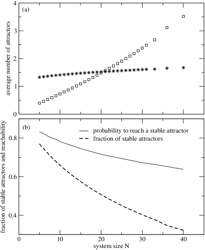
Figure 1: Frequency and accessibility of stable and unstable cycles in Kauffman networks. (a) Average number of stable ($\ast$) and unstable ($\Box$) attractors as a function of the number of nodes in the network. (b) Fraction of initial conditions leading to a stable attractor (solid line) and the ratio between numbers of stable and all attractors (dashed line). Data points in (a) are averages over $R$ independent realizations of the Kauffman network, $R=10^{7}$ for $N<24$, $R=10^{6}$ for $24\leq N\leq 31$ and $R=10^{4}$ otherwise. For increasing computational speed the networks are subject to the decimation procedure Bilke01 before simulation. For the decimated network we fully enumerate the state space such that it is certain that all cycles are detected. Sizes of basins of attraction in (b) have been estimated in $10^{5}$ networks, testing 100 randomly chosen initial conditions in each original network (no decimation applied).

Let us study a Kauffman network composed of $N$ binary nodes where each node determines its state $x_{i}$ by applying a Boolean function (a rule table) $f_{i}:\{0,1\}^{2}\rightarrow\{0,1\}$ on inputs received from two other nodes $a(i)$ and $b(i)$, according to a randomly chosen quenched topology. To be definite, we exclude self-couplings. Starting from an arbitrary initial condition $(x_{1}(0),x_{2}(0),\dots,x_{N}(0))$, states of the nodes are synchronously updated at integer times $t$ according to the Boolean function

$$x_{i}(t+1)=f_{i}(x_{a(i)}(t),x_{b(i)}(t)).$$ (1)

The network itself as defined by $f_{i}$, $a(i)$, and $b(i)$ remains constant in time. Running the system from a randomly chosen initial condition, its finite discrete state space of $2^{N}$ possible states ensures that, eventually, a state reappears that has been encountered before. From thereon, the deterministic system will indefinitely follow the attractor it reached (which is either a periodic limit cycle or a fixed point). Different initial conditions may lead to the same or to a different attractor. The total number of attractors is a characteristic property of a network. The expected number of cycles in an ensemble of random Kauffman networks has been shown to increase superpolynomially with system size $N$ Samuelsson03 .

Let us now define a criterion for stability of an attractor in the presence of deviations from deterministic parallel update. For this purpose, we replace the discrete update times by a continuous time variable $t$ where nodes may update at any point in time. Our goal is to slightly desynchronize the dynamics of the network by shifting the individual updates of nodes to slightly earlier or later time points. To avoid that this generates spurious spikes during transitional phases (e.g. when several signals interact that used to be simultaneous, but now arrive at slightly different times), nodes have to be prevented from switching on a time scale $s$ much shorter than the original integer update time step (i.e., $s\ll 1$). This is implemented by a low pass filter that averages out fluctuations on short characteristic times scales $s$, namely by averaging over the input signal according to

$$x_{i}(t+1)=\Theta\left[(2s)^{-1}\int_{t-s}^{t+s}f_{i}(x_{a(i)}(t),x_{b(i)}(t)){\rm d}t-1/2\right]$$ (2)

where $\Theta$ is the step function with $\Theta(h)=1$ for $h\geq 0$ and $\Theta(h)=0$ otherwise. Let us briefly check how this works. Imagine node $a(i)$ switches on at time $t$, node $b(i)$ switches off at time $t+\epsilon$, while $f_{i}$ is the function and. Without low pass filter ($s=0$), node $i$ switches on at time $t+1$ and off again at time $t+1+\epsilon$. When the switching time scale $s$ of nodes is sufficiently slowed down, $s>\epsilon$, the spurious spike is filtered out, i.e. node $i$ remains constant. Note that in the limit of fast switching time scale $s\rightarrow 0$, Eq. (2) converges towards Eq. (1). In particular, all synchronous solutions of Eq. (1), i.e. solutions with nodes switching precisely at integer values of $t$, are solutions of Eq. (2) for arbitrary $s<1/2$, as well.

Starting from such a synchronous attractor of a network, let us now perturb it at some time $T$ by temporarily retarding parts of the switching events. Thereby, a subset of nodes that would normally change state at time $T$ is kept frozen in their present state during the time interval $[T,T+\epsilon]$ with $\epsilon<s$. After $t=T+\epsilon$, we let the system evolve as usual according to Eq. (2). Note that the original and the perturbed solution differ only on time intervals $[t,t+\epsilon[$ for integer $t$. In general, the time lag may propagate, i.e. for each integer $t\geq T$ some units flip at time $t$ while others flip at time $t+\epsilon$ in the perturbed solution. If, however, there is a later integer time $t^{\ast}>T$ such that either no flips occur at time $t^{\ast}$ or no flips happen at time $t^{\ast}+\epsilon$, the perturbation has been overcome and the system has regained synchrony. We call an attractor stable if for all possible perturbations of the above type (i.e. for all possible permutations of perturbed and non-perturbed nodes) the system regains synchrony and the original attractor is stabilized within a finite time interval. Otherwise the attractor is called unstable. In real world situations with continuous noise, such unstable attractors will accumulate phase shifts that eventually shift the system into some other, stable attractor.

With this we here choose a particularly simple criterion for the stability of an attractor in a Boolean network. The system is on a stable attractor if after each small perturbation it reaches the attractor again where, as a minimal perturbation, a small deceleration or acceleration of a switching event is used. On unstable attractors, such time lags do not relax. Thus, ongoing perturbations eventually lead to a change in time ordering of the switching events and the system reaches a different attractor. Note that this scenario is much better suited as a stability criterion than stochastically adding or removing switching events Qu02 ; Amaral04 , which does not allow for the limit of infinitesimally weak perturbations. The low pass filter characteristics used here is further motivated by the dynamics of biochemical switches Rao02 where molecule concentrations typically respond slowly, leading to an overall low-pass filter characteristics of the switch. Low pass filter characteristics is a natural property of genes and is a simple means of stabilization which is of low cost and ubiquitous in nature. We here model this mechanism as an effective time average over the input signal that suppresses short pulses. Note that under synchronous update of the model networks, pulses cannot be shorter than unit time such that the filter can be neglected.

Applying the robustness criterion to random Boolean networks at criticality, one observes that the average number of all attractors, stable and unstable ones, grows much faster than the average number of stable attractors alone (see Fig. 1(a)). In large networks, almost all attractors are expected to be unstable. Interestingly, the probability to reach a stable attractor from a random initial condition is much larger than the fraction of stable attractors, as shown in Fig. 1(b). Thus, unstable attractors typically have significantly smaller basins of attraction than stable attractors.

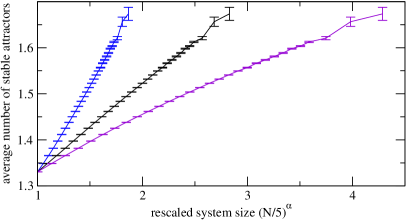
Figure 2: System size scaling of the number of stable attractors. Plotted as a function of the rescaled number of nodes $(N/5)^{\alpha}$ with $\alpha=0.3,0.5,0.7$ (left to right). Error bars in (b) indicate standard deviation divided by $\sqrt{R}$ with ensemble size $R$ (cf. Fig. 1).

The main result is that, with system size $N$, the number of stable attractors grows sublinearly as $\sim N^{\alpha}$ with $\alpha\approx 0.5$, as shown in Fig. 2. A least squares fit of the form $c+bN^{\alpha}$ fits best ($\langle\chi^{2}\rangle=0.00013$) with the parameter values $\alpha=0.448$, $c=1.107$, and $b=0.108$ (with a correlation coefficient for this fit of $r=0.999742$).

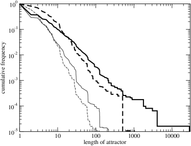
Figure 3: Statistics of attractor lengths for networks with $N=10$ (thin curves) and $N=30$ (thick curves). The cumulative distribution is shown for stable attractors (solid lines) and unstable attractors (dashed lines). For $N=10$ nodes the average length of stable attractors is $\langle l\rangle_{\rm nat}=2.59$, of unstable attractors $\langle l\rangle_{\rm art}=3.56$; for $N=30$ we find $\langle l\rangle_{\rm nat}=5.50$ and $\langle l\rangle_{\rm art}=7.16$.

Further let us analyze the number $l$ of states contained in the attractors. While stable attractors are shorter on average than unstable attractors, the distribution of attractor lengths is broader for stable than for unstable attractors, as shown in Fig. 3. The majority of long attractors with lengths far above average are stable.

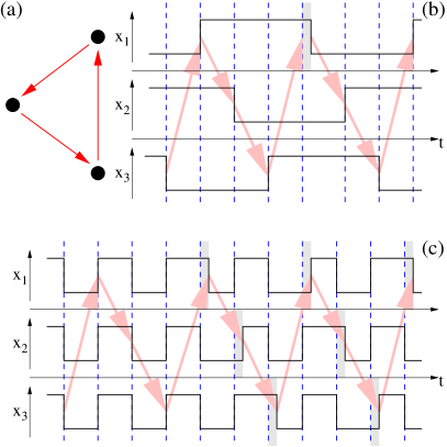
Figure 4: A stable and an unstable attractor in the same system. (a) Three nodes forming a directed cycle (feedback loop). Each node $i$ performs the Boolean function negation on the input from its predecessor $j$, i.e. $x_{i}(t+1)=1-x_{j}(t)$. (b) Temporal evolution of a stable attractor. There is a unique causal chain of flipping events (thick arrows). A retarded update (shaded box) retards all subsequent events by the same amount of time. Thus perturbations heal immediately. (c) Unstable attractor. It can be interpreted as the superposition of three independent chains of flipping events propagating along the cycle of nodes. One of the chains is indicated by thick arrows as in (b). Retarding an event effects subsequent events in the same causal chain only. Causal chains remain phase shifted. The system does not regain synchrony after a perturbation. See reference Klemm04 for a detailed analysis of attractor stability in small systems.

Can we understand by a simple picture how unstable attractors differ from stable ones? Most obviously, unstable attractors occur when the network falls into two or more non-interacting clusters. When all updates in one of the clusters are delayed by the time $\epsilon$, this phase lag with respect to all other clusters cannot heal. All attractors with flipping events in more than one network cluster are unstable. However, also in networks consisting of a single cluster (more precise: with a single strongly connected component) unstable attractors are found. Figure 4 illustrates the coexistence of a stable and an unstable attractor in a small connected network. The example suggests that an attractor is stable if there is a single cascade of switching events. Let us consider the minimal number of simultaneous flipping events

$$m=\min_{t}|\{i|x_{i}(t)\neq x_{i}(t+1)\}|$$ (3)

for a given attractor. The attractors with $m=0$ are the fixed points. These are stable by definition because no flipping events are to be retarded. Attractors with $m=1$ are stable as well. These attractors contain a step with only a single flipping event. Going through this step the system always regains synchrony. For $m\geq 2$ the attractor is likely to contain several chains of causal events as in Fig. 4(c). In the simulations we find that a large fraction $u$ of the attractors with $m\geq 2$ is unstable, $u=0.856,0.882,0.899,0.9094$ for $N=10,20,30,36$, respectively. Thus the minimal number of simultaneous flipping events $m$ allows for an almost perfect distinction between stable and unstable attractors. Note that $m$ is measured in the decimated networks Bilke01 .

Comparing these results to past studies of random Boolean networks at criticality ($K=2$ inputs per node), we obtain a distinctly different picture: Only a small fraction of all attractors are at all stable against small amounts of noise. Or, put differently, the effect of spurious synchronization due to a parallel update mode has been underestimated in previous studies, at least where these studies have been made with a potential application to biological systems in mind. In particular, characteristic properties of the attractor statistics are different when considering the subset of stable attractors: The average number of stable attractors scales less than linearly while the number of unstable attractors shows a faster, superlinear growth with $N$. Also, stable attractors have a significantly larger basin of attraction than unstable ones. One may speculate that this latter property might have been the reason for the long prevalence of the opinion that the total number of attractors scales as $\sqrt{N}$ Kauffman93 . Mainly these stable attractors were likely to be found in the early studies using sparse sampling.

If one aims at discussing Boolean networks as simple models for biological systems, our study suggests to consider more carefully the question of which attractors are at all relevant to the biological system. For example, Kauffman’s observation of the number of attractors in critical random Boolean networks exhibiting a similar scaling with system size as the number of cell types with genome size in organisms Kauffman93 seems to be wrong in the light of the results by Troein and Samuelsson Samuelsson03 . However, it appears to be still open to debate when considering solely the subset of stable attractors.

Acknowledgement We thank Barbara Drossel, Albert Diaz-Guilera, Leon Glass, and Björn Samuelsson for helpful comments. This work was supported by the Deutsche Forschungsgemeinschaft DFG.

References

- (1) S.A. Kauffman, J. Theor. Biol. 22, 437 (1969).
- (2) L. Glass and S.A. Kauffman, J. Theor. Biol. 39, 103 (1973).
- (3) S.A. Kauffman, The Origins of Order. (Oxford University Press, New York, 1993)
- (4) For a review see for example The chipping forecast II, Nature Genetics Supplement 32, 461-552 (2002).
- (5) M. Aldana, S. Coppersmith and L.P. Kadanoff in Perspectives and Problems in Nonlinear Science, edited by E. Kaplan, J.E. Marsden, and K.R. Sreenivasan (Springer, New York, 2003).
- (6) S. Bilke and F. Sjunnesson, Phys. Rev. E 65, 016129 (2001).
- (7) B. Samuelsson and C. Troein, Phys. Rev. Lett. 90, 098701 (2003).
- (8) B. Drossel, T. Mihaljev, F. Greil, preprint cond-mat/0410579
- (9) B. A. Huberman, N. S. Glance, Proc. Natl. Acad. Sci. USA 90, 7716 (1993).
- (10) M.Y. Choi and B.A. Huberman, Phys. Rev. B 28, 2547 (1983)
- (11) T.E. Ingerson and R.L. Buvel, Physica D 10, 59 (1984).
- (12) R.J. Bagley and L. Glass, J. Theor. Biol. 183 269 (1996).
- (13) I. Harvey and T. Bossomaier, Proceedings of the Fourth European Conference on Artificial Life (ECAL97), pp. 67-75 (MIT Press, 1997).
- (14) K. Klemm, S. Bornholdt, preprint q-bio/0309013 (2003).
- (15) X. Qu, M. Aldana and L.P. Kadanoff, J. Stat. Phys. 109 967, (2002).
- (16) L. A. N. Amaral, A. Díaz-Guilera, A. A. Moreira, A. L. Goldberger, and L. A. Lipsitz, Proc. Natl. Acad. Sci. USA 101, 15551 (2004).
- (17) C.V. Rao, D.M. Wolf, and A.P. Arkin, Nature 420, 231-237 (2002).
- (18) K. Klemm, S. Bornholdt, preprint q-bio/0409022 (2003).