Dynamical corrections to the DFT-LDA electron conductance in nanoscale systems

Abstract

Using time-dependent current-density functional theory, we derive analytically the dynamical exchange-correlation correction to the DC conductance of nanoscale junctions. The correction pertains to the conductance calculated in the zero-frequency limit of time-dependent density-functional theory within the adiabatic local-density approximation. In particular, we show that in linear response the correction depends non-linearly on the gradient of the electron density; thus, it is more pronounced for molecular junctions than for quantum point contacts. We provide specific numerical examples to illustrate these findings.

Recent attempts to apply static density-functional theory HK_KS (DFT) to electronic transport phenomena in nanoscale conductors have met with some success. Typical examples are atomic-scale point contacts, where the conductance, calculated with DFT within the local-density approximation (LDA), is found to be in excellent agreement with the experimental values Jan . When applied to molecular junctions, however, similar calculations have not been so successful, yielding theoretical conductances typically larger than their experimental counterparts DiVentra00 . These discrepancies have spurred research that has led to several suggested explanations. One should keep in mind, however, that these quantitative comparisons often neglect some important aspects of the problem. For instance, the experimentally reported values of single-molecule conductance seem to be influenced by the choice of the specific experimental set-up Reed ; Lindsay ; Reichert ; Tao : different fabrication methods lead to different conductances even for the same type of molecule, with recent data appearing to be significantly closer to the theoretical predictions Tao than data reported in earlier measurements Lindsay2 . In addition, several current-induced effects such as forces on ions DiVentra04 and local heating DiVentra03 are generally neglected in theoretical calculations. These effects may actually generate substantial structural instabilities leading to atomic geometries different than those assumed theoretically. However, irrespective of these issues, one is naturally led to ask the more general question of whether static DFT, within the known approximations for the exchange-correlation (xc) functional, neglects fundamental physical information that pertains to a truly non-equilibrium problem. In other words, how accurate is a static DFT calculation of the conductance within the commonly used approximation for the xc functional, LDA, compared to a time-dependent many-body calculation in the zero-frequency limit?

In this Letter we provide an answer to this question. Specifically, we seek to analytically determine the correction to the conductance calculated within the static DFT-LDA approach and illustrate the results with specific examples. A few recent attempts were made in this direction. For instance, Delaney et al. Delaney used a configuration-interaction based approach to calculate currents from many-body wavefunctions. While this scheme seems to yield a conductance for a specific molecule of the same order of magnitude as found in earlier experiments on the same system, it relies on strong assumptions about the electronic distribution of the particle reservoirs Delaney . Following Gonze et al. Gonze , Evers et al. Ever suggested that approximating the xc potential of the true nonequilibrium problem with its static expression is the main source of discrepancy between the experimental results and theoretical values. However, these authors do not provide analytical expressions to quantify their conclusion.

Our system is the nanojunction illustrated in Fig. 1, which contains two bulk electrodes connected by a constriction. In order to understand the dynamical current response, one must formulate the transport problem beyond the static approach using time-dependent density functional theory Runge ; note-closed ; Burke (TDDFT). In the low frequency limit, the so-called adiabatic local-density approximation (ALDA) has often been used to treat time-dependent phenomena in inhomogeneous electronic systems. However, it is essential to appreciate that the dynamical theory includes an additional xc field beyond ALDA Vignale96 – a field that does not vanish in the DC limit. This extra field, when acting on the electrons, induces an additional resistance $R^{\rm dyn}$, which is otherwise absent in the static DFT calculations or TDDFT calculations within the ALDA note-resistance . Our goal is to find an analytic expression for this resistance and then estimate its value in realistic systems. We will show that the dynamical xc field opposes the purely electrostatic field: one needs a larger electric field to achieve the same current, implying that the resistance is, as expected, increased by dynamical xc effects.

Figure 1: Schematic of a nanoscale junction between electrodes with applied bias $V$. Due to dynamical exchange-correlation (xc) effects there is an xc field which gives rise to an additional voltage drop $V^{\rm dyn}$ compared to the electrostatic potential difference.

We proceed to calculate the xc electric field. This quantity was determined by Vignale, Ullrich and Conti using time-dependent current-density functional theory (TDCDFT) Vignale97 ; Ullrich . In their notation, this field is

$$E_{\alpha}({\bf r},\omega)=E_{\alpha}^{ALDA}({\bf r},\omega)-\frac{1}{en}\partial_{\beta}\sigma_{\alpha\beta}({\bf r},\omega),$$ (1)

where $E_{\alpha}^{ALDA}({\bf r},\omega)$ is the ALDA part of the xc contribution, $\sigma_{\alpha\beta}({\bf r},\omega)$ is the xc stress tensor, and $e$ is the electron charge. Here $n=n_{0}({\bf r})$ is the ground-state number density of an inhomogeneous electron liquid. We are interested in the dynamical effects that are related to the second term on the RHS of Eq. (1), i.e.,

$$E_{\alpha}^{\rm dyn}({\bf r},\omega)\equiv-\frac{1}{en}\partial_{\beta}\sigma_{\alpha\beta}({\bf r},\omega).$$ (2)

In the static limit Vignale97 , we can transform $E_{\alpha}^{\rm dyn}$ into an associated potential by integrating between points $a$ and $b$ inside the electrodes lying on the $z$ axis. We take the $z$-direction to be parallel to the current flow. The end points $a$ and $b$ are in regions where the charge density does not vary appreciably, i.e., $\partial_{z}(1/n)|^{b}_{a}\sim 0$ (see Fig. 1). This yields

$$V^{\rm dyn} = -\int_{a}^{b}\lim_{\omega\to 0}\,\mathrm{Re}\,{\bf E}^{\rm dyn}\cdot d{\bf l}$$ (3)

$$= \int_{a}^{b}\frac{1}{en}\lim_{\omega\to 0}\,\mathrm{Re}\,\partial_{\beta}\sigma_{z\beta}({\bf r},\omega)dz.$$

Importantly, we include here only the part of the electric field that varies in phase with the current (i.e., we take the real part of the stress tensor). In general—e.g., at finite frequency—the electric field has both an in-phase (dissipative) and an out-of-phase (capacitive) component, where the latter is related to the shear modulus of the inhomogeneous electron liquid. Such capacitive components play a crucial role in the theory of the dielectric response of insulators. We ignore them here on the basis that they do not contribute to the resistance note-capactive .

The general xc stress tensor in TDCDFT Ullrich is given by

$$\sigma_{\alpha\beta}({\bf r},\omega) = \tilde{\eta}(n,\omega)\left(\partial_{\beta}u_{\alpha}+\partial_{\alpha}u_{\beta}-\frac{2}{3}\nabla\cdot{\bf u}\,\delta_{\alpha\beta}\right)$$ (4)

$$+\tilde{\zeta}\,(n,\omega){\bf\nabla}\cdot{\bf u}\,\delta_{\alpha\beta},$$

where $\tilde{\eta}(n,\omega)$ and $\tilde{\zeta}(n,\omega)$ are the frequency-dependent viscoelastic coefficients of the electron liquid, while ${\bf u}={\bf j}/n$ and ${\bf j}$ are the velocity field and the particle current density, respectively, induced by a small, time-dependent potential.

The viscoelastic coefficients are given by

$$\tilde{\eta}(n,\omega)=-\frac{n^{2}}{i\omega}f^{h}_{xc,T}(\omega)$$ (5)

and

$$\tilde{\zeta}(n,\omega)=-\frac{n^{2}}{i\omega}\left\{f^{h}_{xc,L}(\omega)-\frac{3}{4}f^{h}_{xc,T}(\omega)-\epsilon_{xc}^{\prime\prime}\right\},$$ (6)

where $f^{h}_{xc,L}(\omega)$ and $f^{h}_{xc,T}(\omega)$ are, respectively, the longitudinal and transverse xc kernel of the homogeneous electron gas evaluated at the local electron density $n=n_{0}({\bf r})$, while $\epsilon_{xc}^{\prime\prime}$ is simply

$$\epsilon_{xc}^{\prime\prime}=\left.\frac{d^{2}\epsilon_{xc}(n)}{dn^{2}}\right|_{n_{0}({\bf r})}.$$ (7)

In the representative systems that we examine below, the derivatives in the transverse directions $x$ and $y$ account for only a small fraction of the total dynamical xc field and can hence be ignored. We thus obtain

$$E_{z}=-\frac{1}{en}\partial_{z}\sigma_{zz}.$$ (8)

We then see that

$$\sigma_{zz}=\frac{4\eta}{3}\partial_{z}u_{z}$$ (9)

where the viscosity $\eta=\lim_{\omega\to 0}{\rm Re}\tilde{\eta}(\omega)$ is a function of $n$, and therefore of $z$. The real part of $\tilde{\zeta}(\omega)$ vanishes in the limit of $\omega\to 0$. Under the same assumptions of negligible transverse variation in current density note-j , we can write

$$u_{z}=\frac{I}{enA_{c}}$$ (10)

where $I>0$ is the total current (independent of $z$), and $A_{c}$ is the cross sectional area explain . Substituting this into the equation for the voltage drop and integrating by parts we arrive at

$$V^{\rm dyn}=-\frac{4I}{3e^{2}A_{c}}\int_{a}^{b}\eta\frac{(\partial_{z}n)^{2}}{n^{4}}dz~{}.$$ (11)

Because $\eta$ is positive – a fact that follows immediately from the positivity of energy dissipation in the liquid – we see that the right hand side of this equation is negative-definite: the electrostatic voltage is always opposed by the dynamical xc effect. We identify the quantity on the right hand side of Eq. (11) with $-R^{\rm dyn}I$, where $R^{\rm dyn}$ is the additional resistance due to dynamical effects. According to TDCDFT, the current that flows in the structure in response to an electric potential difference $V$ is given by

$$I=G_{s}(V+V^{\rm dyn})=G_{s}(V-R^{\rm dyn}I)$$ (12)

where $G_{s}$ is the conductance calculated in the absence of dynamical xc effects (e.g., by means of the techniques of Ref. DiVentra01, ). Solving Eq. (12) leads immediately to the following expression for the total resistance $R=V/I$:

$$R=\frac{1}{G_{s}}+R^{\rm dyn}~{},$$ (13)

where

$$R^{\rm dyn}=\frac{4}{3e^{2}A_{c}}\int_{a}^{b}\eta\frac{(\partial_{z}n)^{2}}{n^{4}}dz.$$ (14)

The dynamical xc term thus increases the resistance.

This is the central result of our paper. It shows that the dynamical effects (beyond ALDA) on the resistance depend nonlinearly on the variation of the charge density when the latter changes continously from one electrode to the other across the junction. In a nanojunction, this correction is non-zero only at the junction-electrode interface where the electron density varies most. Knowing the charge density one can then estimate this resistance.

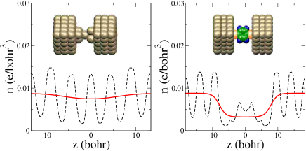
Figure 2: Planar (dashed line) and macroscopic (solid line) averages of the charge density for a gold point contact (left) and a molecular junction (right).

Let us thus consider two specific examples that have attracted much attention, namely the gold point contact and the molecular junction formed by a benzene-dithiolate (BDT) molecule between two bulk electrodes (see insets in Fig. 2) and estimate the error made by the (A)LDA calculation in determining the resistance. In order to make a connection between the microscopic features of these junctions and the density in Eq. (14), we model the charge density $n=n_{0}({\bf r})$ as a product of smoothed step functions in every direction, i.e.,

$$n_{0}({\bf r}) = n_{e}\Xi(z,d,\gamma_{e})$$ (15)

$$+n_{c}\Omega(x,h,\gamma_{c})\Omega(y,w,\gamma_{c})\Omega(z,d,\gamma_{e}).$$

The smoothed step function is given by

$$\Theta(z,l,\gamma)=\frac{1}{e^{(z+l/2)/\gamma}+1},$$ (16)

where $l$ is the full-width at half-maximum and $\gamma$ is the decay length. Here, $\Omega(z,l,\gamma)=\Theta(z,-l,\gamma)-\Theta(z,l,\gamma)$ and $\Xi(z,l,\gamma)=1-\Omega(z,l,\gamma)$; $\Omega(z,l,\gamma)$ represents the density distribution of the junction $n_{c}$, which smoothly connects to the constant bulk density $n_{e}$ of the two electrodes separated by a distance $d$. Finally, $h$ and $w$ represent the lateral dimensions of the junction.

The electron densities are obtained from self-consistent static DFT calculations with the xc functional treated within the LDA Abinit . The (111) gold surface orientation is chosen for both the point contact and the molecular junction (see schematics in Fig. 2).

In Fig 2 we plot the planar and macroscopic averages of the self-consistent electron densities for both systems as a function of distance from the center of the junction along the $z$-direction. The macroscopic average is then fitted to the simple charge model in Eq. (15). The fitted density is then substituted in Eq. (14) to find the correction to the resistance. The estimated value of $R^{\rm dyn}$ note-eta for the point contact is $\sim$0.2 K$\Omega$ (the static DFT resistance is about 12 K$\Omega$ Lager ), while for the BDT molecule is $\sim$40K$\Omega$ (to be compared with the linear response static DFT resistance of about 360 K$\Omega$ DiVentra01 ). As expected, $R^{\rm dyn}$ for BDT is larger than that for the point contact due to the larger variation of the average density between the bulk electrodes and the molecule. In Fig. 3 we plot the resistance in Eq. (14) as a function of the ratio $n_{e}/n_{c}$ and the decay constant $\gamma$, where we fix $n_{e}$ to the value of bulk gold ($r_{s}\approx 3$). The resistances of the two specific examples are indicated by dots in the figure. It is clear that the dynamical contributions to the resistance can become substantial when the gradient of the density at the electrode-junction interface becomes large. These corrections are thus more pronounced in organic/metal interfaces than in nanojunctions formed by purely metallic systems.

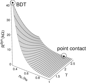
Figure 3: The resistance due to dynamical effects as calculated from Eq. 14 with the charge density determined from DFT-LDA calculations as a function of the main parameters discussed in the text. The resistance of a gold point contact and a BDT molecular junction are indicated by dots.

In summary, we have shown that dynamical effects in the xc potential contribute an additional resistance on top of the static DFT-LDA one. The magnitude of the additional resistance, within linear response and the zero-frequency limit, depends on the gradient of the charge density across the junction. This additional resistance is thus larger in molecular junctions than in quantum point contacts.

We acknowledge financial support from an NSF Graduate Fellowship (MZ), NSF Grant No. DMR-0313681 (GV) and NSF Grant No. DMR-0133075 (MD).

References

- (1) E-mail address: diventra@physics.ucsd.edu
- (2) P. Hohenberg and W. Kohn, Phys. Rev. B 135, 864 (1964); W. Kohn and L. J. Sham, Phys. Rev. 140, A1133 (1965).
- (3) See, e.g., N. Agraït, A. Levy Yeyati and J. M. van Ruitenbeek, Phys. Rep. 377, 81 (2003).
- (4) See, for instance, M. Di Ventra, S. T. Pantelides, and N. D. Lang, Phys. Rev. Lett. 84, 979 (2000); Y. Xue, S. Datta, and M. A. Ratner, J. Chem. Phys. 115, 4292 (2001).
- (5) M. A. Reed et al, Science 278, 252 (1997).
- (6) X. D. Cui et al, Science, 294, 571 (2001).
- (7) J. Reichert et al, Phys. Rev. Lett. 88, 176804 (2002).
- (8) B.Q. Xu and N.J. Tao, Science, 301, 1221 (2003); X.Y. Xiao, B.Q. Xu, and J. Tao, Nano Lett. 4, 267 (2004).
- (9) J. Tomfohr et al, Introducing Molecular Electronics, edited by G. Cuniberti, G. Fagas, K. Richter (Springer, NY, 2004), Chap. 12.
- (10) M. Di Ventra, Y. C. Chen, and T. N. Todorov, Phys. Rev. Lett. 92, 176803 (2004).
- (11) M. J. Montgomery, T. N. Todorov, and A. P. Sutton, J. Phys.: Cond. Mat. 14, 1 (2002); Y. C. Chen, M. Zwolak, and M. Di Ventra, Nano Lett. 3, 1691 (2003).
- (12) P. Delaney and J. C. Greer, Phys. Rev. Lett. 93, 036805 (2004).
- (13) X. Gonze and M. Scheffler, Phys. Rev. Lett. 82. 4416 (1999).
- (14) F. Evers, F. Weigend, and M. Koentopp, Phys. Rev. B 69, 235411 (2004).
- (15) E. Runge and E. K. U. Gross, Phys. Rev. Lett. 52, 997 (1984).
- (16) For a strictly finite and isolated system the true many-body total current is given exactly by the one-electron total current, obtained from TDDFT provided one knows the exact xc functional [M. Di Ventra and T. N. Todorov, J. Phys. Cond. Matt. 16, 8025 (2004); G. Stefanucci and C.-O. Almbladh, Europhys. Lett. 67, 14 (2004)]. Here we ask the question of what percentage of the total conductance originates from dynamical effects beyond ALDA.
- (17) K. Burke, R. Car, and R. Gebauer, cond-mat/0410362.
- (18) G. Vignale and W. Kohn, Phys. Rev. Lett. 77, 2037 (1996). The additional field is a strongly non-local functional of the density, but becomes a local functional when expressed in terms of the current density.
- (19) We implicitly assume that we can identify a physical initial state such that, in the zero-frequency limit, the conductance obtained from a TDDFT calculation within the ALDA for the xc kernel equals the conductance obtained using static DFT within LDA. The assumption requires non-resonant scattering and is thus satisfied by quantum point contacts and molecular junctions in linear response when the Fermi level falls between the highest occupied and the lowest unoccupied molecular orbitals DiVentra00 .
- (20) G. Vignale, C.A. Ullrich, and S. Conti, Phys. Rev. Lett. 79, 4878 (1997).
- (21) C. A. Ullrich and G. Vignale, Phys. Rev. B 65, 245102 (2002).
- (22) In the current-density functional theory, the capacitive effect is described by a static shear modulus. Within the local density approximation for a metallic system, this quantity is expected to vanish in the frequency regime relevant to DC conduction.
- (23) The current density varies much slower than the particle density in the contact region. [See, e.g., N. D. Lang, Phys. Rev. B 36, R8173 (1987).] If we relaxed this approximation, we would obtain a larger value for the dynamical contribution to the resistance.
- (24) Note that we have assumed the right electrode is positively biased (see Fig. 1) so that electrons flow from left to right. The current is thus defined as flowing in the opposite direction.
- (25) M. Di Ventra and N. D. Lang, Phys. Rev. B 65, 045402 (2001).
- (26) The calculations have been performed with the Abinit package (X. Gonze et al, http://www.abinit.org); the present calculations are performed using norm-conserving pseudopotentials. (N. Troullier, J. L. Martins, Phys. Rev. B 43, 1993 (1991).)
- (27) We have used the viscosity where and are the Fermi wave-vector of the bulk electrodes and Bohr radius, respectively.
- (28) J. Lagerqvist, Y. C. Chen and M. Di Ventra, Nanotechnology 15, 459 (2004).