Time-dependent density-functional theory approach to nonlinear particle-solid interactions in comparison with scattering theory

Abstract

An explicit expression for the quadratic density-response function of a many-electron system is obtained in the framework of the time-dependent density-functional theory, in terms of the linear and quadratic density-response functions of noninteracting Kohn-Sham electrons and functional derivatives of the time-dependent exchange-correlation potential. This is used to evaluate the quadratic stopping power of a homogeneous electron gas for slow ions, which is demonstrated to be equivalent to that obtained up to second order in the ion charge in the framework of a fully nonlinear scattering approach. Numerical calculations are reported, thereby exploring the range of validity of quadratic-response theory.

1 Introduction

The inelastic interaction of charged particles with matter is one of the fundamental problems of contemporary physics. It encompasses such phenomena as the stopping power of solids for moving ions, electron and positron energy-loss spectroscopy, inelastic low-energy electron diffraction, and hot-electron dynamics [1, 2].

A fruitful approach to the theoretical treatment of particle-solid interactions has proven to be the use of perturbation series expansions in powers of the projectile-target Coulomb interaction. For the description of many-electron targets, one typically introduces linear and quadratic density-response functions, which describe the electron density induced by external perturbations.

While linear-response theory has proven successful in the description of the interaction of fast projectiles with solids, in the case of low projectile velocities and low electron densities a nonlinear description becomes quantitatively necessary [3, 4, 5]. Besides, there exist phenomena which cannot be explained in the framework of linear-response theory, an example being the existing difference between the scatterings of positively and negatively charged particles [6, 7].

The random-phase approximation (RPA) has served as the natural starting point for the calculation of both linear [8] and quadratic [4, 5] density-response functions of the homogeneous electron gas. However, exchange and correlation (xc) effects, which are absent in the RPA, are known to be important for metallic electron densities [9]. The purpose of this paper is to derive in the framework of the time-dependent density-functional theory (TDDFT) [10, 11] an explicit expression for the quadratic density-response function of a many-electron system, which will then be used to evaluate the second-order energy loss per unit path length of charged particles moving through solid targets, i.e. the so-called stopping power of the target.

Another approach to evaluate the energy loss of slow ions moving in a many-electron system is based on the ordinary formulation of scattering theory. In this approach [12, 13, 14], the stopping power for a heavy particle is determined in the low-velocity limit from the knowledge of the scattering phase-shifts, which can be obtained from a static nonlinearly screened potential by solving self-consistently the Kohn-Sham equation of density-functional theory (DFT) [15]. Since these nonperturbative calculations include all orders in the projectile-target interaction, they represent an important standard to investigate the range of validity of perturbative expansions. Nonetheless, they have the limitation of being restricted to low velocities ($v<<v_{F}$, $v_{F}$ being the Fermi velocity) of recoilless probe particles moving in bulk materials.

The interrelation of the perturbative-response and nonperturbative-scattering approaches in their overlapping range of applicability (low-velocity limit and small projectile charge) is both an interesting and non-trivial problem. The starting points of these two schemes are completely different and there are no grounds to a priori assume equivalence between them. In this paper, we demonstrate that in the low-velocity limit and to second order in the external perturbation our quadratic-response formalism and the scattering approach are equivalent, thereby extending the RPA-based proof reported in Ref. [3] to the general case where the xc effects are included.

This paper is organized as follows. In Sec. 2, we derive in the framework of TDDFT a formally exact explicit expression for the quadratic density-response function of a many-electron system, in terms of the noninteracting Kohn-Sham linear and quadratic density-response functions and functional derivatives of the time-dependent xc potential. In Sec. 3, we derive basic expressions for the stopping power of a uniform electron gas, in the framework of both quadratic-response and nonperturbative-scattering schemes. The results of numerical calculations are presented in Sec. 4. We use atomic units throughout, i.e., $e^{2}=\hbar=m_{e}=1$.

2 Quadratic density response

In the framework of TDDFT, Petersilka et al. [17] demonstrated that within linear-response theory the electron density $n_{1}({\bf r},t)$ induced in an arbitrary interacting many-electron system by the time-dependent external potential $\phi^{ext}({\bf r},t)$ coincides with the electron density induced in the corresponding system of noninteracting Kohn-Sham electrons by the time-dependent effective potential

$$\phi_{1}^{eff}({\bf r},t)=\phi^{ext}({\bf r},t)+\int d{\bf r}^{\prime}\,v({\bf r},{\bf r}^{\prime})\,n_{1}({\bf r}^{\prime},t)$$ (1)

(2)

$$+\int d{\bf r}^{\prime}\int dt^{\prime}\,f_{xc}[n_{0}]({\bf r},t;{\bf r}^{\prime},t^{\prime})\,n_{1}({\bf r}^{\prime},t^{\prime}),$$ (3)

where $v({\bf r},{\bf r}^{\prime})=1/|{\bf r}-{\bf r}^{\prime}|$ is the bare Coulomb potential, and $f_{xc}[n_{0}]({\bf r},t;{\bf r}^{\prime},t^{\prime})$ is the functional derivative of the time-dependent xc potential $V_{xc}[n]({\bf r},t)$ of TDDFT, to be evaluated at the unperturbed static electron density $n_{0}({\bf r})$:

$$f_{xc}[n_{0}]({\bf r},t;{\bf r}^{\prime},t^{\prime})=\left.{\delta V_{xc}[n]({\bf r},t)\over\delta n({\bf r}^{\prime},t^{\prime})}\right|_{n=n_{0}}.$$ (4)

The linear-response scheme reported in Ref. [17] can be extended to all orders in the external perturbation. This has been carried out by Gross et al. [11] in the general case of spatially inhomogeneous electron systems, and self-consistent integral equations for the quadratic and higher order interacting density response functions have been obtained by these authors. In the specific case of the uniform electron gas, which we are here interested in, these equations can be easily solved, to produce explicit interacting density response functions in terms of their noninteracting counterparts and the functional derivatives of the exchange-correlation potential. However, instead of adopting the method of solution of the above mentioned integral equations, we find it more instructive for our purposes, as well as self-contained, to derive an explicit expression for the quadratic density response function considering the uniform case from the very beginning.

The electron density $n_{1}({\bf r},t)+n_{2}({\bf r},t)+\cdots$ induced in an arbitrary many-electron system by the time-dependent external potential $\phi^{ext}({\bf r},t)$ coincides with the electron density induced in the corresponding system of noninteracting Kohn-Sham electrons by the time-dependent effective potential $\phi_{1}^{eff}({\bf r},t)+\phi_{2}^{eff}({\bf r},t)+\cdots$, where $\phi_{1}^{eff}({\bf r},t)$ is given by Eq. (1) and

$$\phi_{2}^{eff}({\bf r},t)=\int d{\bf r}^{\prime}\,v({\bf r},{\bf r}^{\prime})\,n_{2}({\bf r}^{\prime},t)$$ (5)

(6)

$$+\int d{\bf r}^{\prime}\int dt^{\prime}\,f_{xc}[n_{0}]({\bf r},t;{\bf r}^{\prime},t^{\prime})\,n_{2}({\bf r}^{\prime},t)$$ (7)

(8)

$$+\frac{1}{2}\int d{\bf r}^{\prime}\int dt^{\prime}\int d{\bf r}^{\prime\prime}\int dt^{\prime\prime}\,g_{xc}[n_{0}]({\bf r},t;{\bf r}^{\prime},t^{\prime};{\bf r}^{\prime\prime},t^{\prime\prime})$$ (9)

(10)

$$\times n_{1}({\bf r}^{\prime},t^{\prime})\,n_{1}({\bf r}^{\prime\prime},t^{\prime\prime}),$$ (11)

$g_{xc}[n_{0}]({\bf r},t;{\bf r}^{\prime},t^{\prime};{\bf r}^{\prime\prime},t^{\prime\prime})$ being the second functional derivative of the time-dependent xc potential $V_{xc}[n]({\bf r},t)$, to be evaluated at the unperturbed static electron density $n_{0}({\bf r})$:

$$g_{xc}[n_{0}]({\bf r},t;{\bf r}^{\prime},t^{\prime};{\bf r}^{\prime\prime},t^{\prime\prime})=\left.{\delta^{2}V_{xc}[n]({\bf r},t)\over\delta n({\bf r}^{\prime},t^{\prime})\delta n({\bf r}^{\prime\prime},t^{\prime\prime})}\right|_{n=n_{0}}.$$ (12)

In the case of a homogeneous electron gas, there is translational invariance in all directions. Hence, taking Fourier transforms with respect to space and time, the exact momentum and frequency dependent induced electron densities, $n_{1}({\bf q},\omega)$ and $n_{2}({\bf q},\omega)$, can be written as

$$n_{1}(q)=\chi_{1}(q)\phi^{ext}(q)=\chi^{0}_{1}(q)\phi_{1}^{eff}(q)$$ (13)

and

$$n_{2}(q)=\int d^{4}q_{1}\chi_{2}(q,q_{1})\phi^{ext}(q_{1})\phi^{ext}(q-q_{1})=\chi^{0}_{1}(q)$$ (14)

(15)

$$\times\phi_{2}^{eff}(q)+\int d^{4}q_{1}\chi^{0}_{2}(q,q_{1})\phi_{1}^{eff}(q_{1})\phi_{1}^{eff}(q-q_{1}),$$ (16)

where $q=({\bf q},\omega)$, $\phi_{1}^{eff}(q)$ and $\phi_{2}^{eff}(q)$ are Fourier transforms of the time-dependent effective potentials of Eqs. (1) and (5), respectively, $\phi^{ext}(q)$ is the Fourier transform of the external potential, $\chi_{1}(q)$ and $\chi_{2}(q,q_{1})$ denote the exact linear and quadratic density-response functions of the interacting electron system, and $\chi_{1}^{0}(q)$ and $\chi_{2}^{0}(q,q_{1})$ represent the corresponding density-response functions of noninteracting Kohn-Sham electrons. Substituting Eqs. (1) and (5) into Eqs. (13) and (14), one finds

$$\chi_{1}(q)=\tilde{\epsilon}^{-1}(q)\,\chi_{1}^{0}(q)$$ (17)

and

$$\chi_{2}(q,q_{1}) = \tilde{\epsilon}^{-1}(q)\chi_{2}^{0}(q,q_{1})\tilde{\epsilon}^{-1}(q_{1})\tilde{\epsilon}^{-1}(q-q_{1})$$ (18)

$$+ \chi_{1}(q)g_{xc}(q,q_{1})\chi_{1}(q_{1})\chi_{1}(q-q_{1})/2,$$ (20)

where $v(q)=4\pi/{\bf q}^{2}$ is the Fourier transform of the Coulomb potential, $f_{xc}(q)$ and $g_{xc}(q,q_{1})$ denote the Fourier transforms of the xc kernels of Eqs. (4) and (12), and $\tilde{\epsilon}(q)$ is the test-charge–electron dielectric function [18, 19]

$$\tilde{\epsilon}(q)=1-\chi_{1}^{0}(q)\left[v(q)+f_{xc}(q)\right].$$ (21)

The Fourier transforms of the linear and quadratic xc kernels in Eqs. (21) and (18), respectively, are defined as

$$f_{xc}(q) = \int f_{xc}[n_{0}]({\bf r},t;{\bf r}^{\prime},t^{\prime})e^{-i{\bf q}\cdot({\bf r}-{\bf r}^{\prime})+i\omega(t-t^{\prime})}d{\bf r}\,dt,$$

$$g_{xc}(q,q_{1}) = \int g_{xc}[n_{0}]({\bf r},t;{\bf r}^{\prime},t^{\prime};{\bf r}^{\prime\prime},t^{\prime\prime})e^{i[{\bf q}_{1}\cdot({\bf r}^{\prime}-{\bf r})-\omega_{1}(t^{\prime}-t)]}$$

$$\times e^{i[({\bf q}-{\bf q}_{1})\cdot({\bf r}^{\prime\prime}-{\bf r})-(\omega-\omega_{1})(t^{\prime\prime}-t)]}d{\bf r}^{\prime}\,dt^{\prime}\,d{\bf r}^{\prime\prime}\,dt^{\prime\prime}.$$

Equations (17) and (18) generalize the exact linear density response reported in Ref. [17] to the realm of quadratic-response theory and the static quadratic density response reported in Ref. [20] to the general case of a time-dependent perturbation. In the so-called adiabatic LDA (ALDA), which is only rigorous in the long-wavelength (${\bf q}\to 0$) and static ($\omega\to 0$) limits, the xc kernels $f_{xc}(q)$ and $g_{xc}(q,q_{1})$ are simply the first and second derivatives with respect to the unperturbed density of the static xc potential of a uniform electron gas: $V^{\prime}_{xc}(n_{0})$ and $V^{\prime\prime}_{xc}(n_{0})$. In the RPA, the xc kernels $f_{xc}(q)$ and $g_{xc}(q,q_{1})$ are set equal to zero. Finally, we find our theory in agreement with that of Ref. [11], while the homogeneity of the system we consider enables us to obtain the explicit quadratic density-response function of Eq. (18) instead of presenting the results in the form of self-consistent integral equations.

3 Stopping power

There are two routes to describe the stopping power of the homogeneous electron gas. One is based on a perturbative expansion of the density response of the target (appropriate for arbitrary projectile velocities) and the other on the knowledge of the phase shifts of potential scattering of electrons by a statically screened impurity (only valid for low projectile velocities). We first consider these two alternative approaches, then we focus on the overlapping range of their applicability, by considering the low-velocity limit of the quadratic-response formulation and a second-order expansion of the transition-matrix elements of potential scattering.

3.1 Quadratic density response

To third order in the projectile charge $Z_{1}$, the average energy lost per unit length traveled by a recoilless probe particle moving with velocity v in a homogeneous electron gas, i.e., the so-called stopping power of the target is obtained as follows [21, 22]

$$-\frac{dE}{dx} = -2\,\frac{Z_{1}^{2}}{\pi v}\int d{\bf q}\,\frac{{\bf q}\cdot{\bf v}}{\textbf{q}^{2}}\,\left[\frac{{\rm Im}\,\chi_{1}(q)}{\textbf{q}^{2}}\right.$$ (22)

$$+ \left.\frac{Z_{1}}{2\pi^{2}}\int\frac{d{\bf q}_{1}}{\textbf{q}_{1}^{2}|{\bf q}-{\bf q}_{1}|^{2}}\,{\rm Im}\,\chi_{2}(q,q_{1})\right],$$ (24)

which by virtue of Eqs. (17) and (18) can be rigorously expressed as

$$-\frac{dE}{dx}=-2\,\frac{Z_{1}^{2}}{\pi v}\,{\rm Im}\int d{\bf q}\,\frac{{\bf q}\cdot{\bf v}}{\textbf{q}^{2}}\,\left\{\frac{\chi^{0}_{1}(q)\,\tilde{\epsilon}^{-1}(q)}{\textbf{q}^{2}}+\frac{Z_{1}}{2\pi^{2}}\int\frac{d{\bf q}_{1}}{\textbf{q}_{1}^{2}|{\bf q}-{\bf q}_{1}|^{2}}\right.\times$$ (25)

(26)

$$\left.\tilde{\epsilon}^{-1}(q)\,\tilde{\epsilon}^{-1}(q_{1})\,\tilde{\epsilon}^{-1}(q-q_{1})\left[\chi^{0}_{2}(q,q_{1})+\chi^{0}_{1}(q)g_{xc}(q,q_{1})\chi^{0}_{1}(q_{1})\chi^{0}_{1}(q-q_{1})/2\right]\right\},$$ (27)

where now $q=({\bf q},{\bf q}\cdot{\bf v})$ and $q_{1}=({\bf q}_{1},{\bf q}_{1}\cdot{\bf v})$.

3.1.1 Low-velocity limit

At low frequencies we can write [8]

$${\rm Im}\,\chi^{0}_{1}(q)=\omega\,A_{\bf q}$$

and [5]

$${\rm Im}\,\chi_{2}^{0}(q,q_{1})=\omega\,B_{{\bf q},{\bf q}_{1}}+\omega_{1}\,B_{{\bf q}_{1},{\bf q}}+(\omega-\omega_{1})\,B_{{\bf q}-{\bf q}_{1},-{\bf q}_{1}},$$

where

$$A_{\bf q} = -\frac{\Theta(2k_{F}-q)}{2\pi q},$$

$$B_{{\bf q},{\bf q}_{1}} = 2\,A_{\bf q}\,\frac{\left(1-k_{F}^{2}/q_{R}^{2}\right)^{-1/2}}{|{\bf q}_{1}||{\bf q}-{\bf q}_{1}|}$$

$$\times {\rm sgn}\,(\cos\phi_{\bf q})\Theta(q_{R}-k_{F}).$$

Then in the ALDA one finds

$$-\frac{dE}{dx}=-2\frac{Z_{1}^{2}}{\pi v}\int d{\bf q}\frac{({\bf q}\cdot{\bf v})^{2}}{\textbf{q}^{2}}\left\{\frac{A_{\bf q}\,\tilde{\epsilon}_{\bf q}^{-2}}{\textbf{q}^{2}}+\frac{Z_{1}}{\pi^{2}}\int\frac{d{\bf q}_{1}}{\textbf{q}_{1}^{2}|{\bf q}_{1}-{\bf q}|^{2}}\right.$$ (28)

(29)

$$\times\left.\left[\tilde{\epsilon}_{\bf q}^{-1}\,B_{{\bf q},{\bf q}_{1}}\tilde{\epsilon}_{{\bf q}_{1}}^{-1}\tilde{\epsilon}_{{\bf q}-{\bf q}_{1}}^{-1}+C_{\bf q}\tilde{\epsilon}_{\bf q}^{-2}\chi^{0}_{2,({\bf q},{\bf q}_{1})}\tilde{\epsilon}^{-1}_{{\bf q}_{1}}\tilde{\epsilon}^{-1}_{{\bf q}-{\bf q}_{1}}+V^{\prime\prime}_{xc}\,A_{\bf q}\tilde{\epsilon}^{-2}_{\bf q}\,\chi_{1,{\bf q}_{1}}\,\chi_{1,{\bf q}-{\bf q}_{1}}/2,\right]\right\}.$$ (30)

Here

$$C_{\bf q}=(v_{\bf q}+V^{\prime}_{xc})\,A_{\bf q},$$

$v_{\bf q}=4\pi/{\bf q}^{2}$ is the Fourier transform of the Coulomb potential, $k_{F}$ is the Fermi momentum, $\chi_{1,{\bf q}}$ and $\chi_{2,({\bf q},{\bf q}_{1})}^{0}$ denote the static ($\omega=0$) linear interacting and quadratic noninteracting density-response functions, respectively, $\tilde{\epsilon}_{\bf q}$ is the static test-charge–electron dielectric function, $\Theta(x)$ is the Heaviside step function, $q_{R}$ is the radius of the circle circumscribing the triangle formed by the vectors ${\bf q}$, ${\bf q}_{1}$, and ${\bf q}-{\bf q}_{1}$, and $\phi_{\bf q}$ represents the angle facing ${\bf q}$ in this triangle. Evaluating some of the integrals in Eq. (30), one finds

$$-\frac{1}{v}\,\frac{dE}{dx}=\frac{4Z_{1}^{2}}{3\pi}\int\limits_{0}^{2k_{F}}dq\left\{\frac{1}{q\,\tilde{\epsilon}^{2}_{\bf q}}+\frac{2Z_{1}q}{\pi}\int_{0}^{\infty}dq_{1}\int_{-1}^{1}d\mu\frac{1}{|\textbf{q}-\textbf{q}_{1}|^{2}\tilde{\epsilon}_{\bf q}\tilde{\epsilon}_{{\bf q}_{1}}\tilde{\epsilon}_{{\bf q}-{\bf q}_{1}}}\right.$$ (31)

$$\times\left.\left[\frac{(v_{\bf q}+V_{xc}^{\prime})\chi^{0}_{2,({\bf q},{\bf q}_{1})}+V_{xc}^{\prime\prime}\chi^{0}_{1,{\bf q}_{1}}\chi^{0}_{1,{\bf q}-{\bf q}_{1}}/2}{\tilde{\epsilon}_{\bf q}}+\frac{2\,\Theta(q_{R}-k_{F})}{q_{1}|{\bf q}-{\bf q}_{1}|\sqrt{1-k_{F}^{2}/q_{R}^{2}}}\,{\rm sgn}(\cos\phi_{\bf q})\right]\right\},$$

where $q$ and $q_{1}$ now denote the magnitude of ${\bf q}$ and ${\bf q}_{1}$, respectively, and $\mu=\cos\phi_{{\bf q}-{\bf q}_{1}}$. If we put $V^{\prime}_{xc}=V^{\prime\prime}_{xc}=0$ in Eq. (31), we retrieve the RPA result of Ref. [5]. If we keep the actual value of $V^{\prime}_{xc}$ but still putting $V^{\prime\prime}_{xc}=0$, we reproduce the calculations reported in Ref. [9].

3.2 Potential scattering

In the low-velocity limit of a recoilless probe particle of charge $Z_{1}$, the interaction between the Fermi gas and the probe particle can be represented as the elastic scattering of independent electrons by a Kohn-Sham effective static central potential $V(r)$. Hence, the average energy loss per unit path length of a recoilless charged particle moving with velocity ${\bf v}$ ($v<<v_{F}$) through a uniform electron gas of density $n_{0}$ is given by the following expression:

$$-\frac{dE}{dx}=n_{0}v\,k_{F}\sigma_{tr}(k_{F}),$$ (32)

where

$$\sigma_{tr}(k)={16\pi^{5}\over k^{4}}\int_{0}^{2k}dq\,q^{3}|T_{fi}|^{2}$$ (33)

is the so-called transport cross section, $T_{fi}$ denoting the transition-matrix element [23]:

$$T_{fi}=<\phi_{{\bf k}_{f}}|V|\psi_{{\bf k}_{i}}>.$$ (34)

Here, $\phi_{\bf k}$ and $\psi_{\bf k}$ represent noninteracting and interacting electron wave functions, respectively, ${\bf k}_{i}$ and ${\bf k}_{f}$ denote the electron momentum before and after the collision, $k=|{\bf k}_{i}|=|{\bf k}_{f}|$ is the magnitude of the electron momentum, ${\bf q}={\bf k}_{f}-{\bf k}_{i}$ is the momentum transfer, and $V(r)$ is taken to be the Kohn-Sham effective potential

$$V(r)=-\frac{Z_{1}}{r}+\int\frac{n(r^{\prime})}{|{\bf r}-{\bf r}^{\prime}|}\,d{\bf r}^{\prime}+V_{xc}(r),$$ (35)

$n(r)$ being the electron density induced by the presence of the static probe particle and $V_{xc}(r)$ being the xc potential at point ${\bf r}$ of the inhomogeneous electron system, which in the LDA is simply the xc potential of a homogeneous electron gas with electron density $n(r)$. The well known expression of the transport cross-section in terms of the phase-shifts $\delta_{l}(k)$ of the scattering problem in the spherically symmetric potential

$$\sigma_{tr}(k)=\frac{4\pi}{k^{2}}\sum\limits_{l=0}^{\infty}(l+1)\sin^{2}[\delta_{l}(k)-\delta_{l+1}(k)],$$ (36)

greatly facilitates the numerical calculations, while the Friedel sum rule [24]

$$Z_{1}=\frac{2}{\pi}\sum\limits_{l=0}^{\infty}(2l+1)\delta_{l}(k_{F})$$ (37)

is helpful in controlling self-consistency. Echenique et al. [12, 13] and Nagy et al. [14] evaluated the LDA Kohn-Sham effective potential by solving self-consistently the Kohn-Sham equation of DFT, and then computed the stopping power from Eqs. (32) and (36).

We proceed by considering a second-order perturbative expansion of the transition matrix $T_{fi}(q)$ entering Eq. (33), which will then allow us to derive $Z_{1}^{2}$- and $Z_{1}^{3}$- contributions to the stopping power from Eq. (32).

The Born series for the transition matrix element $T_{fi}$ in powers of the effective potential $V(r)$ [which can be expanded in powers of the bare interaction $-Z_{1}/r$: $V_{1}(r)+V_{2}(r)\cdots$] is obtained as follows

$$T_{fi}=\langle\phi_{{\bf k}_{f}}|\,V+VG_{k}^{0}V+\cdots\,|\phi_{{\bf k}_{i}}\rangle,$$ (38)

where $G^{0}_{k}({\bf r},{\bf r}^{\prime})$ is the noninteracting Green’s function

$$G_{k}^{0}({\bf r},{\bf r}^{\prime})=-{1\over 2\pi}\,{\rm e}^{ik|{\bf r}-{\bf r}^{\prime}|}/|{\bf r}-{\bf r}^{\prime}|.$$

Up to third order in the charge $Z_{1}$ of the probe particle, the square of the transition matrix element of Eq. (38) yields

$$|T_{fi}|^{2}=\left[V_{1}({\bf q})\right]^{2}+2\,V_{1}({\bf q})$$ (39)

$$\times \left[V_{2}({\bf q})+P\int d{\bf q}_{1}\frac{V_{1}({\bf q}_{1})V_{1}({\bf q}-{\bf q}_{1})}{{\bf k}_{i}^{2}/2-({\bf k}_{i}-{\bf q}_{1})^{2}/2}\right],$$ (41)

where

$$V_{1}(\textbf{q})=-\frac{Z_{1}}{2\pi^{2}q^{2}}+(v_{\bf q}+V^{\prime}_{xc})\,n_{1}(\textbf{q})$$ (42)

and

$$V_{2}(\textbf{q}) = (v_{\bf q}+V^{\prime}_{xc})\,n_{2}(\textbf{q})$$ (43)

$$+ \frac{V^{\prime\prime}_{xc}}{2}\int d{\bf q}_{1}\,n_{1}({\bf q}_{1})\,n_{1}({\bf q}-{\bf q}_{1}),$$ (45)

$n_{1}({\bf q})$ and $n_{2}({\bf q})$ being the linear and quadratic induced electron densities, and $P$ in Eq. (39) denoting that the principal value of the integral must be taken at the point where the integrand is singular. It is interesting to notice that the second-order ($Z_{1}^{3}$) contribution to $|T_{fi}|^{2}$ has two sources. One is the first Born contribution to the quadratically screened effective potential $V(r)$ and the other is the second Born contribution to the linearly screened effective potential, as pointed out in Ref. [3]. They have opposite signs and it is the latter which dominates [3, 4, 5].

Substituting Eqs. (13) and (14) into Eqs. (42) and (43) and then substituting the expansion of Eq. (39) into Eq. (33), one finds from Eq. (32) the following expansion for the stopping power:

$$-\frac{1}{v}\,\frac{dE}{dx}=\frac{4}{3\pi}\int\limits_{0}^{2k_{F}}dq\left\{\frac{Z_{1}^{2}}{q\tilde{\epsilon}^{2}_{\bf q}}+\frac{Z_{1}^{3}q}{\pi^{2}}\int\frac{d{\bf q}_{1}}{q_{1}^{2}|\textbf{q}-\textbf{q}_{1}|^{2}\tilde{\epsilon}_{\bf q}\tilde{\epsilon}_{{\bf q}_{1}}\tilde{\epsilon}_{{\bf q}-{\bf q}_{1}}}\right.$$ (46)

(47)

$$\times\left.\left[\frac{(v_{\bf q}+V_{xc}^{\prime})\chi^{0}_{2,({\bf q},{\bf q}_{1})}+V_{xc}^{\prime\prime}\,\chi^{0}_{1,{\bf q}_{1}}\,\chi^{0}_{1,{\bf q}-{\bf q}_{1}}/2}{\tilde{\epsilon}_{\bf q}}+\frac{2}{k_{F}^{2}-({\bf k}_{F}-{\bf q}_{1})^{2}}\right]\right\}.$$ (48)

Performing the integration over the angular variables of ${\bf q}_{1}$, one readily reproduces Eq. (31), thereby proving the equivalence between the quadratic-response and potential-scattering schemes in the limit of low velocities of the probe particle. This generalizes the RPA analysis reported in Ref. [3] to the general situation where xc effects are taken into account.

4 Results of numerical calculations

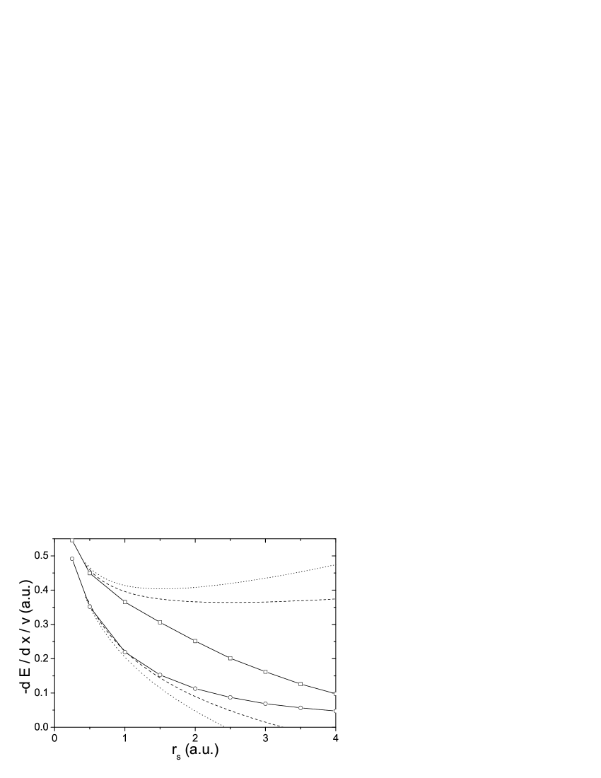
Figure 1: Stopping power of a uniform electron gas in the low-velocity limit, divided by the projectile velocity (friction coefficient), as a function of the electron-density parameter $r_{s}$. The chained curves represent nonperturbative potential-scattering LDA calculations for protons (squares) and antiprotons (circles). The dashed (dotted) line represents ALDA calculations to third order in the projectile charge $Z_{1}$ with (without) inclusion of the second derivative $V^{\prime\prime}_{xc}$ of the xc potential.

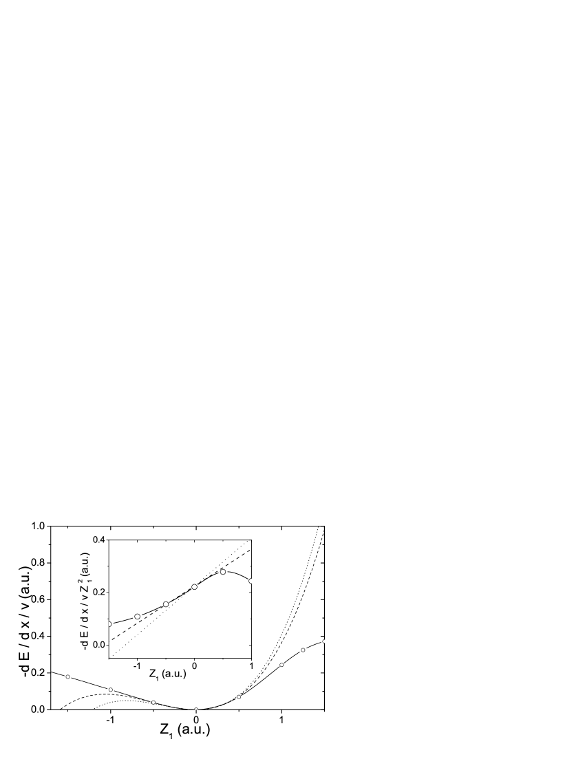
Figure 2: Stopping power of a uniform electron gas in the low-velocity limit, divided by the projectile velocity (friction coefficient), as a function of the projectile charge $Z_{1}$ and for the electron-density parameter $r_{s}=2.07$ corresponding to the average electron density of valence electrons in Al. The chained curve represents nonperturbative potential-scattering LDA calculation. The dashed (dotted) line represents our ALDA calculations to third order in the projectile charge $Z_{1}$ with (without) inclusion of the second derivative $V^{\prime\prime}_{xc}$ of the xc potential. The inset shows the same plots normalized to the square of the projectile’s charge.

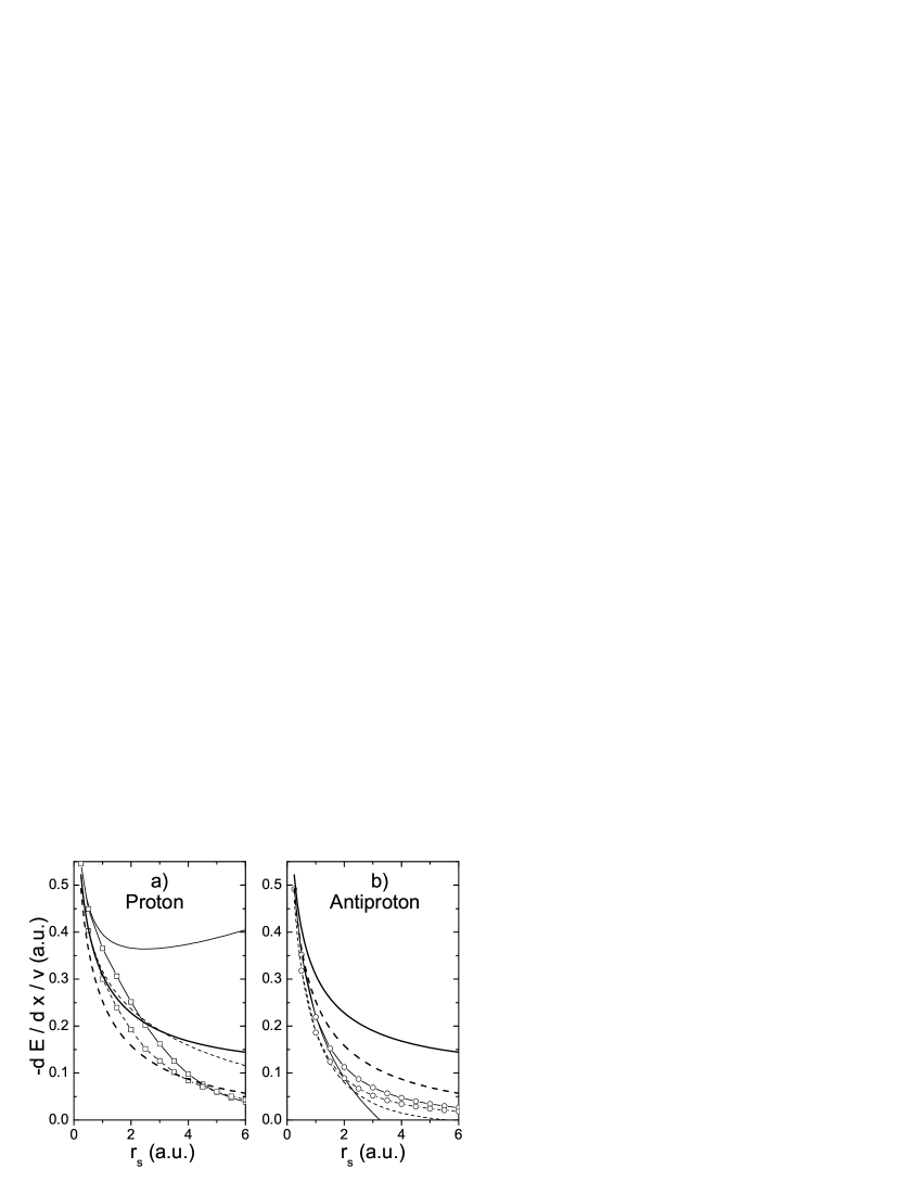
Figure 3: Stopping power of a uniform electron gas in the low-velocity limit, divided by the projectile velocity (friction coefficient) and as a function of the electron-density parameter $r_{s}$, for protons (a) and antiprotons (b). Solid (dashed) curves represent calculations including (omitting) exchange and correlation. The chained curves represent the nonperturbative potential-scattering calculations. Bold (both solid and dashed) lines are linear ($Z_{1}^{2}$) contributions. Thin (both solid and dashed) lines represent quadratic ($Z_{1}^{3}$) calculations.

In Fig. 1 we plot the stopping power of a uniform electron gas of density $n_{0}$ in the low-velocity limit, divided by the projectile velocity (friction coefficient), for protons ($Z_{1}=1$) and antiprotons ($Z_{1}=-1$) as a function of the electron-density parameter $r_{s}=(3/4\pi n_{0})^{1/3}$. We evaluate both the perturbative expansion of Eq. (31) and the non-perturbative formula by using the Perdew-Zunger [25] parametrization of the xc potential of a uniform electron gas. Our non-perturbative calculations reproduce those reported in Refs. [13] and [14] for protons and antiprotons, respectively. Perturbative and nonperturbative calculations are also plotted in Fig. 2, but now for the electron-density parameter $r_{s}=2.07$ corresponding to valence electrons in Al and as a function of the projectile charge $Z_{1}$.

Also plotted in Figs. 1 and 2 are perturbative calculations with no inclusion of the second derivative of the xc potential $V_{xc}$, as reported in Ref. [9], showing that the inclusion of this term brings the perturbative calculations very close to the full nonlinear calculation in the range of high electron densities (small $r_{s}$) and small projectile charges. Figure 1 shows that the quadratic (perturbative) stopping power for antiprotons is extremely accurate for all electron densities with $r_{s}\leq 2$. Figure 2 shows that in the case of Al target ($r_{s}=2.07$) and negative projectile charges the quadratic stopping power is accurate for the antiproton charge ($Z_{1}=-1$) and above, but it is only accurate for small positive values of the projectile charge ($Z_{1}\leq 0.5$). This is due to the presence of the truly bound electronic states and the behavior of resonances in the case of a positive probe particle, which are only included in a fully nonlinear scheme.

To elucidate the role of resonances, we have performed the numerical analysis of the phase-shifts $\delta_{l}(k)$ of the scattering in the self-consistent potential (35). At a given $r_{s}$ with growing $Z_{1}$ a resonance, which always exists in the continuum spectrum, moves to lower energy and grows both sharper and more intense, which results in a stronger variation of the phase-shifts. Since the density of states is proportional to the derivative of the phase-shifts $\delta^{\prime}_{l}(k)$, the low-lying continuum states get filled preferentially resulting, similarly to the occupation of the bound states, in the more efficient screening of the ion charge and eventually in the decrease of the stopping power even before the formation of the bound states. On the other hand, at smaller values of $Z_{1}$ the existence of weak broad resonances at high energies does not affect the applicability of the quadratic theory.

In order to investigate the interplay between high-order interactions and xc effects, we have plotted in Fig. 3 the results of linear ($Z_{1}^{2}$), quadratic ($Z_{1}^{3}$), and fully nonlinear potential-scattering calculations of the stopping power of slow protons and antiprotons, both in the absence and in the presence of xc effects. This figure shows that: (i) The impact of xc effects is considerably larger within linear and quadratic response theory than in the more realistic nonperturbative potential-scattering approach, especially so in the case of protons, which indicates that there must be a large degree of cancelation between first, second and higher-order xc effects. (ii) At high electron densities ($r_{s}\to 0$), the inclusion of xc effects brings the quadratic-response calculations (thin solid lines of Fig. 3) into nice agreement with their DFT based potential-scattering counterparts (chained solid lines). However, xc effects decrease the radius of convergence of the asymptotic perturbative expansion; while an unphysical negative stopping power is obtained within RPA for antiprotons at $r_{s}>5.5$, this unphysical behavior is obtained in the presence of xc effects at $r_{s}>3.2$. (iii) The performance of the perturbative expansion is considerably better for antiprotons than for protons. This can be attributed to the existence of electronic bound states and the behavior of resonances around a moving proton [13], which are out of the reach of the perturbative description. (iv) The performance of the quadratic response theory for the stopping power is considerably better than in the case of the electron density induced at the position of the projectile [26, 27], which is a highly nonlinear magnitude. This is due to the fact that the stopping power involves an integration of the induced density over the whole space, as discussed in Ref. [26].

Finally, we note that apart from the obvious usefulness of quadratic-response calculations in situations where the interaction can be considered to be weak, it has been recently shown that perturbative calculations can be successfully used as input in a variational theory of charged particles interacting with a many-body system. Recent investigations have shown that this new variational theory brings the RPA quadratic stopping power for slow antiprotons into nice agreement with the corresponding nonperturbative potential-scattering calculations for all electron densities [28].

5 Summary and conclusions

We have derived an explicit expression for the quadratic density-response function of a many-electron system in the framework of TDDFT, in terms of the linear and quadratic density-response functions of noninteracting Kohn-Sham electrons and functional derivatives of the time-dependent xc potential. This expression generalizes the rigorous linear density-response function reported in Ref. [17] to the realm of quadratic-response theory, and they satisfy the self-consistent integral equations of Gross et al. [11], valid for arbitrary inhomogeneous electron system.

The exact expression for the quadratic density-response function has been used to obtain the stopping power of a uniform electron gas to second order in the projectile charge $Z_{1}$, which in the low-velocity limit and within the adiabatic LDA is demonstrated to be equivalent to that obtained up to third order in $Z_{1}$ in the framework of a fully nonlinear LDA potential-scattering approach. This generalizes the RPA analysis reported in Ref. [3] to the general situation where xc effects are taken into account.

We have carried out LDA numerical calculations of the stopping power of a uniform electron gas for slow positively and negatively charged ions, as a function of both the electron-density parameter and the projectile charge. We find that quadratic-response theory yields a stopping power that is in excellent agreement with the nonperturbative stopping power in the range of high electron densities and small projectile charges. The quadratic-response (perturbative) stopping power for antiprotons is found to be extremely accurate for all electron densities higher than the electron density of valence electrons in Al. In the case of Al, quadratic-response theory is found to yield accurate results for small negative projectile charges up to the antiproton charge, but a fully nonlinear scheme is required to account for the energy loss of slow protons.

Although our equation (25) for the stopping power is exact to the $Z_{1}^{3}$ order, in the numerical calculations we have utilized the local and adiabatic approximation for the linear and quadratic exchange-correlation kernels, which is consistent with the available fully nonlinear calculations within the potential scattering method. To study the role of the non-locality (wave-vector dependence of the exchange-correlation potential) and non-adiabaticity (its frequency dependence) in the nonlinear theory of stopping-power is, however, a challenging task, and this work is now in progress [29].

References

References

- [1] Echenique P M, Flores F and Ritchie R H 1990 Solid State Phys. 43 229
- [2] Liebsch A 1997 Electronic excitations at metal surfaces (New-York: Plenum)
- [3] Hu C D and Zaremba E 1988 Phys. Rev. B 37 9268
- [4] Pitarke J M, Ritchie R H, Echenique P M and Zaremba E 1993 Europhys. Lett. 24 613
- [5] Pitarke J M, Ritchie R H and Echenique P M 1995 Phys. Rev. B 52 13883
- [6] Barkas W H, Birnbaum W and Smith F M 1956 Phys. Rev. 101 778
- [7] Møller S P, Csete A, Ichioka T, Knudsen H, Uggerhøj U I and Andersen H H 2002 Phys. Rev. Lett. 88 193201
- [8] Lindhard J 1954 K. Dan. Vidensk. Selsk. Mat.-Fys. Medd. 28 1
- [9] del Rio Gaztelurrutia T and Pitarke J M 2000 Phys. Rev. B 62 6862
- [10] Runge E and Gross E K U 1984 Phys. Rev. Lett. 52 997
- [11] Gross E K U, Dobson J F and Petersilka M 1996 Density functional theory of time-dependent phenomena, Density Functional Theory II. Topics of Current Chemistry vol 181 (Berlin: Springer) p 81
- [12] Echenique P M, Nieminen R M and Ritchie R H 1981 Solid State Commun. 37 779
- [13] Echenique P M, Nieminen R M, Ashley J C and Ritchie R H 1986 Phys. Rev. A 33 897
- [14] Nagy I, Arnau A, Echenique P M and Zaremba 1989 Phys. Rev. B 40 11983
- [15] Kohn W and Sham L J 1965 Phys. Rev. 140 A1133
- [16] Salin A, Arnau A, Echenique P M and Zaremba E 1999 Phys. Rev. B 59 2537
- [17] Petersilka M, Gossmann U J and Gross E K U 1996 Phys. Rev. Lett. 76 1212
- [18] Kukkonen C A and Overhauser A W 1979 Phys. Rev. B 20 550
- [19] Echenique P M, Pitarke J M, Chulkov E V and Rubio A 2000 Chem. Phys. 251 1
- [20] Louis A A and Ashcroft N W 1998 Phys. Rev. Lett. 81 4456
- [21] del Rio Gaztelurrutia T. and Pitarke J M 2001 J. Phys. A: Math. Gen. 34 7607
- [22] Nazarov V U and Nishigaki S 2002 Phys. Rev. B 65 94303
- [23] Taylor J R 1972 Scattering theory (New York: John Wiley & Sons)
- [24] Kittel C 1963 Quantum theory of solids (New York: Wiley)
- [25] Perdew J P and Zunger A 1981 Phys. Rev. B 23 5048
- [26] Bergara A, Campillo I, Pitarke J M and Echenique P M 1997 Phys. Rev. B 56 15654
- [27] Arbo D G, Gravielle M S and Miraglia J E 2001 Phys. Rev. A 64 22902
- [28] Nazarov V U, Nishigaki S and Pitarke J M to be published
- [29] Nazarov V U, Pitarke J M, Kim C S and Takada Y to be published