Theoretical investigations for shot noise in correlated resonant tunneling through a quantum coupled system

Abstract

In this paper, we carry out a theoretical analysis of the zero-frequency and finite-frequency shot noise in electron tunneling through a two-level interacting system connected to two leads, when a coherent coupling between the two levels is present, by means of recently developed bias-voltage and temperature dependent quantum rate equations. For this purpose, we generalize the traditional generation-recombination approach for shot noise of two-terminal tunneling devices properly to take into account the coherent superposition of different electronic states (quantum effects). As applications, analytical and numerical investigations have been given in detail for two cases: (1) electron tunneling through a quantum dot connected to ferromagnetic leads with intradot spin-flip scattering, and (2) spinless fermions tunneling through seriesly coupled quantum dots, focusing on the shot noise as functions of bias-voltage and frequency.

I INTRODUCTION

In recent years the study of shot noise in mesoscopic quantum systems has become an emerging topic in mesoscopic physics, because measurement of shot noise can reveal more information of transport properties which are not available through the conductance measurement alone.Blanter ; Beenakker For example, dynamic correlations in the tunneling current originated from the Pauli exclusion principle can provide information regarding the barrier geometry. On the other hand, strong Coulomb blockade effect also acts in correlating wavepackets and shot noise, when the charging energy becomes larger than the thermal energy in small quantum devices.

Besides, special interest has recently been put upon investigation of tunneling through two-level system (TLS), when the coherent coupling between the two levels is presented. In such internally coupled system, quantum interference effects between the two levels play a crucial role in its transport, inducing, for instance, temporal damped oscillations in average current and a corresponding fine structure in shot noise power spectrum $S(\omega)$ due to its intrinsic Rabi oscillation.Wiel ; Gurvitz ; Sun ; Brahim ; Fedichkin ; Gurvitz2 ; Aguado ; Engel Furthermore, it is predicted that a dip or a peak shown in $S(\omega)$ at the Rabi frequency reflects the differing relative phase of states carrying the tunneling current.GurvitzIEEE

In literature, the quantum rate equations have been developed to describe this kind of quantum coherence effects in quantum tunneling through TLS, in associated with the strong Coulomb blockade effect.Nazarov ; Gurvitz1 So far, most calculations for shot noise in TLS have been based on the number-resolved version of quantum rate equations, which takes numbers of tunneled electrons through TLS as parameters of density matrix elements (the degree of freedom of reservoirs), and have made use of Laplace transform to calculate the current-current correlation functions. Unfortunately, this scheme is only valid at zero temperature and high bias-voltage condition.Brahim ; Fedichkin ; Gurvitz2 ; GurvitzIEEE Therefore, it is quite desirable to find a way of evaluating current correlation in arbitrary bias-voltages, particularly in moderately small bias-voltage region, where the coherence plays a more prominent role in quantum tunneling processes. Accordingly, the purpose of this paper is to develop a general scheme to study quantum shot noise spectrum of coupled small quantum systems based on the recently established quantum rate equations with a bias-voltage and temperature dependent version.Dong

Actually, a numerical method, named generation-recombination approach, was established for analysis of shot noise in two-terminal single-electron tunneling devices with the classical rate equation (classical shot noise) in Refs. [Hershfield, ; Korotkov, ; Hanke, ]. These earlier papers proposed a powerful method to evaluate the double-time current correlation function by switching the time-dependent current to a time evolution propagator of the density matrices in a consistent way. In the present paper we will modify this traditional approach to suit the underlying quantum rate equations for properly accounting for the quantum coherence effects, i.e., the nondiagonal elements of density matrix, in calculation of quantum shot noise and develop a tractable computation technique in matrix form.

The rest of this paper is organized as follows. In section II, we study the quantum shot noise for an interacting quantum dot (QD) connected to ferromagnetic leads with intradot spin-flip scattering. First we review the model Hamiltonian for this internally coupled TLS and the underlying quantum rate equations for description of coherent tunneling in sequential picture. Subsequently, we elaborate the general formalism for the quantum shot noise in matrix form and present a convenient numerical method for the matrix calculation in frequency space with the help of the spectral decomposition technique. In the final part of this section, we analyze the zero-frequency Fano factor, which quantifies correlations of shot noise with respect to its uncorrelated Poissonian value, in several limits, and then provide numerical results for the Fano factor as functions of bias-voltage and frequency. In section III, we employ the same procedure to evaluate the quantum shot noise in two coupled quantum dots in series (CQD). Finally, a brief summary is presented in section IV.

II Shot noise in a SINGLE QUANTUM DOT with intradot spin-flip scattering

II.1 Model and quantum rate equations

The system that we study is a single QD with an arbitrary intradot Coulomb interaction $U$ connected with two ferromagnetic leads. In this paper, we assume that the tunneling coupling between the dot and the leads is weak enough to guarantee no Kondo effect and that the QD is in the Coulomb blockade regime. This kind of spin-related single-electron devices suffers inevitably intrinsic relaxations (decoherence) due to the spin-orbital interactionFedichkin or the hyperfine-mediated spin-flip transition.Erlingsson For simplicity, we model the intrinsic spin relaxation with a phenomenological spin-flip term $R$ and assume that this spin-flip process happens solely within the dot (the spin is conserved during tunneling).

Moreover, we assume that the temperature is low enough for one to see the effects due to the discrete charging and discrete structure of the energy levels, i.e. $k_{B}T\ll U$, $\Delta$ ($\Delta$ is the energy spacing between orbital levels). Each of the two leads is separately in thermal equilibrium with the chemical potential $\mu_{\eta}$, which is assumed to be zero in the equilibrium condition and is taken as the energy reference throughout the paper. In the nonequilibrium case, the chemical potentials of the leads differ by the applied bias-voltage $V$. We are interested in the region $eV\ll\Delta$, where only one dot level $(\epsilon_{d})$ contribute to the transport. Here we neglect Zeeman splitting of the level due to weak magnetic fields $B$ ($g\mu_{B}B<k_{B}T)$, which means that both the spin-up and spin-down currents through the dot go through the same orbital level $\epsilon_{d}$. Therefore, the Hamiltonian of resonant tunneling through a single QD can be written as:Dong

$$H = \sum_{\eta,k,\sigma}\epsilon_{\eta k\sigma}c_{\eta k\sigma}^{\dagger}c_{\eta k\sigma}^{{\phantom{\dagger}}}+\epsilon_{d}\sum_{\sigma}c_{d\sigma}^{\dagger}c_{d\sigma}^{{\phantom{\dagger}}}+R(c_{d\uparrow}^{\dagger}c_{d\downarrow}^{{\phantom{\dagger}}}$$ (2)

$$+c_{d\downarrow}^{\dagger}c_{d\uparrow}^{{\phantom{\dagger}}})+Un_{d\uparrow}n_{d\downarrow}+\sum_{\eta,k,\sigma}(V_{\eta\sigma}c_{\eta k\sigma}^{\dagger}c_{d\sigma}^{{\phantom{\dagger}}}+{\rm{H.c.}}),$$

where $c_{\eta k\sigma}^{\dagger}$ ($c_{\eta k\sigma}$) and $c_{d\sigma}^{\dagger}$ ($c_{d\sigma}$) are the creation (annihilation) operators for electrons with momentum $k$, spin-$\sigma$ and energy $\epsilon_{\eta k\sigma}$ in the lead $\eta$ ($\eta={\rm L,R}$) and for a spin-$\sigma$ electron on the QD, respectively. $n_{d\sigma}=c_{d\sigma}^{\dagger}c_{d\sigma}^{{\phantom{\dagger}}}$ is the occupation operator in the QD. The fourth term describes the Coulomb interaction among electrons on the QD. The fifth term represents the tunneling coupling between the QD and the reservoirs. We assume that the coupling strength $V_{\eta\sigma}$ is spin-dependent to take into account the ferromagnetic leads.

Under the assumption of weak coupling between the QD and the leads, and with the application of the wide band limit in the two leads, electronic transport through this system in sequential regime can be described by the bias-voltage and temperature dependent quantum rate equations for the dynamical evolution of the density matrix elements:Dong

$$\dot{\rho}_{00}=\sum_{\eta\sigma}(\Gamma_{\eta\sigma}^{-}\rho_{\sigma\sigma}-\Gamma_{\eta\sigma}^{+}\rho_{00}),$$ (4a)

$$\dot{\rho}_{\sigma\sigma} = \sum_{\eta}\Gamma_{\eta\sigma}^{+}\rho_{00}+\sum_{\eta}\widetilde{\Gamma}_{\bar{\eta\sigma}}^{-}\rho_{dd}-\sum_{\eta}(\Gamma_{\eta\sigma}^{-}+\widetilde{\Gamma}_{\eta\bar{\sigma}}^{+})\rho_{\sigma\sigma}$$ (4b)

$$+iR(\rho_{\sigma\bar{\sigma}}-\rho_{\bar{\sigma}\sigma}),$$

$$\dot{\rho}_{\sigma\bar{\sigma}}=iR(\rho_{\sigma\sigma}-\rho_{\bar{\sigma}\bar{\sigma}})-\frac{1}{2}\sum_{\eta}(\widetilde{\Gamma}_{\eta\sigma}^{+}+\widetilde{\Gamma}_{\eta\bar{\sigma}}^{+}+\Gamma_{\eta\sigma}^{-}+\Gamma_{\eta\bar{\sigma}}^{-})\rho_{\sigma\bar{\sigma}},$$ (4c)

$$\dot{\rho}_{dd}=\sum_{\eta}\widetilde{\Gamma}_{\eta\downarrow}^{+}\rho_{\uparrow\uparrow}+\sum_{\eta}\widetilde{\Gamma}_{\eta\uparrow}^{+}\rho_{\downarrow\downarrow}-\sum_{\eta}(\widetilde{\Gamma}_{\eta\uparrow}^{-}+\widetilde{\Gamma}_{\eta\downarrow}^{-})\rho_{dd},$$ (4d)

($\sigma=\uparrow,\downarrow$ stands for electron spin and $\bar{\sigma}$ is the spin opposite to $\sigma$). The statistical expectations of the diagonal elements of the density matrix, $\rho_{ii}$ ($i=\{0,\sigma,d\}$), give the occupation probabilities of the resonant level in the QD as follows: $\rho_{00}$ denotes the occupation probability that central region is empty, $\rho_{\sigma\sigma}$ means that the QD is singly occupied by a spin-$\sigma$ electron, and $\rho_{dd}$ stands for the double occupation by two electrons with different spins. Note that they must satisfy the normalization relation $\rho_{00}+\rho_{dd}+\sum_{\sigma}\rho_{\sigma\sigma}=1$. The non-diagonal elements $\rho_{\sigma\bar{\sigma}}$ describe the coherent superposition of different spin states. These temperature-dependent tunneling rates are defined as $\Gamma_{\eta\sigma}^{\pm}=\Gamma_{\eta\sigma}f_{\eta}^{\pm}(\epsilon_{d})$ and $\widetilde{\Gamma}_{\eta\sigma}^{\pm}=\Gamma_{\eta\sigma}f_{\eta}^{\pm}(\epsilon_{d}+U)$, where $\Gamma_{\eta\sigma}$ are the tunneling constants, $f_{\eta}^{+}(\omega)=\{1+e^{(\omega-\mu_{\eta})/T}\}^{-1}$ is the Fermi distribution function of the $\eta$ lead and $f_{\eta}^{-}(\omega)=1-f_{\eta}^{+}(\omega)$. Here, $\Gamma_{\eta\sigma}^{+}$ ($\Gamma_{\eta\sigma}^{-}$) describes the tunneling rate of electrons with spin-$\sigma$ into (out of) the QD from (into) the $\eta$ lead without the occupation of the $\bar{\sigma}$ state. Similarly, $\widetilde{\Gamma}_{\eta\sigma}^{+}$ ($\widetilde{\Gamma}_{\eta\sigma}^{-}$) describes the tunneling rate of electrons with spin-$\sigma$ into (out of) the QD, when the QD is already occupied by an electron with spin-$\bar{\sigma}$, exhibiting the modification of the corresponding rates due to the Coulomb repulsion. The particle current $I_{\eta}$ flowing from the lead $\eta$ to the QD is

$$I_{\eta}/e=\sum_{\sigma}(\widetilde{\Gamma}_{\eta\sigma}^{-}\rho_{dd}+\Gamma_{\eta\sigma}^{-}\rho_{\sigma\sigma}-\widetilde{\Gamma}_{\eta\bar{\sigma}}^{+}\rho_{\sigma\sigma}-\Gamma_{\eta\sigma}^{+}\rho_{00}).$$ (5)

This formula demonstrates that the current is primarily determined by the diagonal elements of the density matrix of the central region. However, the nondiagonal element of the density matrix is coupled with the diagonal elements in the rate equation (4b), and therefore indirectly influences the tunneling current.

II.2 Quantum shot noise formula

There is a well-established procedure, namely, the generation-recombination approach for multielectron channels, for the calculation of the noise power spectrum based on the classical rate equations (classical shot noise).Hershfield ; Korotkov ; Hanke In this section we modify this approach in order to take into account the nondiagonal density matrix elements and derive the general expression for a quantum shot noise for the single QD.

It is well known that the noise power spectra can be expressed as the Fourier transform of the current-current correlation function:

$$S_{I_{\eta}I_{\eta^{\prime}}}(\omega) = 2\int_{-\infty}^{\infty}dte^{i\omega t}[\langle I_{\eta}(t)I_{\eta^{\prime}}(0)\rangle-\langle I_{\eta}\rangle\langle I_{\eta^{\prime}}\rangle]$$ (6)

$$= 2\langle I_{\eta}(t)I_{\eta^{\prime}}(0)\rangle_{\omega}-2\langle I_{\eta}\rangle_{\omega}\langle I_{\eta^{\prime}}\rangle_{\omega}.$$

Here, $I_{\eta}$ and $I_{\eta^{\prime}}$ are the electrical currents across the $\eta$ and $\eta^{\prime}$ junctions and $t$ is the time.

Before proceeding with investigation of current correlation, it is helpful to rewrite the quantum rate equations as matrix form:

$$\frac{d{\bm{\rho}}(t)}{dt}=\mathbf{M}\ {\bm{\rho}}(t)\ ,$$ (7)

where ${\bm{\rho}}(t)=(\rho_{00},\rho_{\uparrow\uparrow},\rho_{\downarrow\downarrow},\rho_{dd},\rho_{\uparrow\downarrow},\rho_{\downarrow\uparrow})^{T}$ is a vector whose components are the density matrix elements, and the $6\times 6$ matrix ${\bf M}$ can be easily obtained from Eqs. (4). Therefore, the statistical averaging of an any time-dependent operator $\hat{A}(t)$ should be replaced by the summation over all elements in this new ${\bm{\rho}}(t)$ representation:

$$\langle\hat{A}(t)\rangle={\rm Tr}\{\hat{A}\rho\}=\sum_{k}[{\bm{A}}{\bm{\rho}}(t)]_{k},$$ (8)

in which ${\bm{A}}$ is the matrix expression of the operator $\hat{A}$ under the basis $(\rho_{00},\rho_{\uparrow\uparrow},\rho_{\downarrow\downarrow},\rho_{dd},\rho_{\uparrow\downarrow},\rho_{\downarrow\uparrow})^{T}$, and the summation goes over all vector $[{\bm{A}}{\bm{\rho}}(t)]$ elements ($k=1,2,\cdots,6$). Correspondingly, we can write the average electrical currents across the left ($I_{L}$) and right ($I_{R}$) junctions at time $t$ as:

$$\langle I_{L(R)}(t)\rangle=e\sum_{k}\left[\hat{\Gamma}_{L(R)}{\bm{\rho}}(t)\right]_{k},$$ (9)

where $\hat{\Gamma}_{L}$ and $\hat{\Gamma}_{R}$ are current operators and the summation goes over all vector $[\hat{\Gamma}_{L(R)}{\bm{\rho}}(t)]$ elements ($k=1,2,\cdots,6$). The current operators contain the rates for tunneling across the left and right junctions respectively,Hershfield and they can be read from Eq. (5) as follows: $\tilde{\Gamma}_{\eta\sigma}^{-}$ describes the tunneling rate of an electron with spin-$\sigma$ out of the QD, when the QD were previously occupied by two electrons. After this tunneling event, QD become singly occupied by a spin-$\bar{\sigma}$ electron. In the other words, $\tilde{\Gamma}_{\eta\sigma}^{-}$ is a transition rate from $\rho_{dd}$ to the $\rho_{\bar{\sigma}\bar{\sigma}}$. It increases occupation probability $\rho_{\bar{\sigma}\bar{\sigma}}$ [this can be also seen by looking the second term of Eq. (4b)] and decreases occupation probability $\rho_{dd}$ [the last term in Eq. (4d)]. The term $\Gamma_{\eta\sigma}^{-}\rho_{\sigma\sigma}$ in Eq. (5) represents the tunneling of $\sigma$ electron out of the QD which leaves QD empty and $\Gamma_{\eta\sigma}^{-}$ can be interpreted as a transition rate from $\rho_{\sigma\sigma}$ to the $\rho_{00}$. In similar way, $\tilde{\Gamma}_{\eta\bar{\sigma}}^{+}$ describes the transition rate from $\rho_{\bar{\sigma}\bar{\sigma}}$ to the $\rho_{dd}$ and $\Gamma_{\eta\sigma}^{+}$ is a transition rate from $\rho_{00}$ to the $\rho_{\sigma\sigma}$. In the basis $(\rho_{00},\rho_{\uparrow\uparrow},\rho_{\downarrow\downarrow},\rho_{dd},\rho_{\uparrow\downarrow},\rho_{\downarrow\uparrow})^{T}$ , the current operators have a matrix form:

$$\hat{\Gamma}_{\eta}=\pm\left(\begin{array}[]{cccccc}0&\Gamma_{\eta\uparrow}^{-}&\Gamma_{\eta\downarrow}^{-}&0&0&0\\ -\Gamma_{\eta\uparrow}^{+}&0&0&\tilde{\Gamma}_{\eta\downarrow}^{-}&0&0\\ -\Gamma_{\eta\downarrow}^{+}&0&0&\tilde{\Gamma}_{\eta\uparrow}^{-}&0&0\\ 0&-\tilde{\Gamma}_{\eta\downarrow}^{+}&-\tilde{\Gamma}_{\eta\uparrow}^{+}&0&0&0\\ 0&0&0&0&0&0\\ 0&0&0&0&0&0\\ \end{array}\right),$$ (10)

where the sign of the current is chosen to be positive when the direction of the current is from left to right, so that the $+$ sign in the last equation is for $\eta=L$ and the $-$ sign stands for $\eta=R$. The stationary current can be obtained as:

$$I=e\sum_{k}\left[\hat{\Gamma}_{L}{\bm{\rho}}^{(0)}\right]_{k}=e\sum_{k}\left[\hat{\Gamma}_{R}{\bm{\rho}}^{(0)}\right]_{k},$$ (11)

where ${\bm{\rho}}^{(0)}$ is the steady state solution of Eq. (7) and which can be obtained from:

$$\mathbf{M}{\bm{\rho}}^{(0)}=0,$$ (12)

along with the normalization relation $\sum_{n=1}^{4}{\bm{\rho}}^{(0)}_{n}=1$. We would like to point out that in our quantum version of rate equations, it is easy to check $\sum_{n}{\bf M}_{nm}=0\ (m=1,2,3,4)$, which implies that: 1) the Matrix ${\bf M}$ has a zero eigenvalue; 2) there is always a steady state solution ${\bm{\rho}}^{(0)}$; 3) the normalization relation $\sum_{n=1}^{4}{\bm{\rho}}_{n}(t)=1$ is independent on time.

A convenient way to evaluate the double-time correlation function Eq (6) is to define the propagator $\hat{T}(t)=\exp[{\bf M}t]$, which governs the time evolution of the density matrix elements ${\bm{\rho}}_{k}(t)$. The average value of the electrical currents across the left ($I_{L}$) and the right ($I_{R}$) junctions at a time $t$ is given by:

$$\langle{I_{L(R)}(t)}\rangle=-e\sum_{k}\left[\hat{\Gamma}_{L(R)}\hat{T}(t){\bm{\rho}}^{(0)}\right]_{k},$$ (13)

which allows us to switch the time evolution from the vector ${\bm{\rho}}(t)$ to the current operators. Thus, we identify $\hat{\Gamma}_{L(R)}(t)=\hat{\Gamma}_{L(R)}\hat{T}(t)$ as the time-dependent current operators. With these time-dependent operators we can calculate correlation functions of two current operators taken at different moments in time. In particular, correlation function of the currents $I_{\eta}$ and $I_{\eta^{\prime}}$ in the tunnel junctions $\eta$ and $\eta^{\prime}$, measured at the two times $t$ and $0$ respectively, is given by:Hershfield

$$\langle{I_{\eta}(t)I_{\eta^{\prime}}(0)}\rangle = \theta(t)\sum_{k}[\hat{\Gamma}_{\eta}(t)\hat{\Gamma}_{\eta^{\prime}}{\bm{\rho}}^{(0)}]_{k}$$

$$+ \theta(-t)\sum_{k}[\hat{\Gamma}_{\eta^{\prime}}(-t)\hat{\Gamma}_{\eta}{\bm{\rho}}^{(0)}]_{k}$$

$$= \theta(t)\sum_{k}[\hat{\Gamma}_{\eta}\hat{T}(t)\hat{\Gamma}_{\eta^{\prime}}{\bm{\rho}}^{(0)}]_{k}$$ (15)

$$+ \theta(-t)\sum_{k}[\hat{\Gamma}_{\eta^{\prime}}\hat{T}(-t)\hat{\Gamma}_{\eta}{\bm{\rho}}^{(0)}]_{k},$$ (16)

where $\theta(t)$ is the Heaviside function and the two terms in Eq. (16) stand for $t>0$ and for $t<0$. The Fourier transform of propagator $\hat{T}(\pm t)$ is $\hat{T}(\pm\omega)=\left(\mp i\omega\hat{I}-\bf{M}\right)^{-1}\$, where $\hat{I}$ is an unit matrix. We can further simplify this expression by using the spectral decomposition of the matrix $\bf{M}$:

$$\mathbf{M}=\sum_{n}\lambda_{n}\mathbf{S}\mathbf{E}^{(nn)}\mathbf{S}^{-1}=\sum_{\lambda}\lambda\hat{P}_{\lambda},$$ (17)

in which $\lambda$ are eigenvalues of the matrix $\bf{M}$, $\mathbf{S}$ is a matrix whose columns are eigenvectors of $\bf{M}$, $\mathbf{E}^{(nn)}$ is a matrix that has $1$ at $nn$ place and all other elements are zeros, and $\hat{P}_{\lambda}$ is a projector operator associated with the eigenvalue $\lambda$, so that $\hat{T}(\pm\omega)$ is

$$\hat{T}(\pm\omega)=\sum_{\lambda}\frac{\hat{P}_{\lambda}}{\mp i\omega-\lambda}.$$ (18)

Inserting expression for propagator $\hat{T}$ into Eq. (16) current-current correlation in the $\omega$-space becomes

$$\langle I_{\eta}(t)I_{\eta^{\prime}}(0)\rangle_{\omega} = \sum_{\lambda,k}\left[\frac{\hat{\Gamma}_{\eta}\hat{P}_{\lambda}\hat{\Gamma}_{\eta^{\prime}}}{{-i\omega-\lambda}}{\bm{\rho}}^{(0)}\right]_{k}$$ (19)

$$+ \sum_{\lambda,k}\left[\frac{\hat{\Gamma}_{\eta^{\prime}}\hat{P}_{\lambda}\hat{\Gamma}_{\eta}}{{i\omega-\lambda}}{\bm{\rho}}^{(0)}\right]_{k}.$$ (20)

Eventually, substituting Eq. (19) into the noise definition Eq. (6), and noting that in the summation over eigenvalues the zero-eigenvalue contribution is canceled exactly by the term $\langle I_{\eta}\rangle\langle I_{\eta^{\prime}}\rangle$, we can obtain the final expression for a noise power spectrum:

$$S_{I_{\eta}I_{\eta^{\prime}}}(\omega)=\delta_{\eta\eta^{\prime}}S^{\rm Sch}_{\eta}$$

$$+2\sum_{k,\lambda\neq 0}\left(\frac{\left[\hat{\Gamma}_{\eta}\hat{P}_{\lambda}\hat{\Gamma}_{\eta^{\prime}}{\bm{\rho}}^{(0)}\right]_{k}}{{-i\omega-\lambda}}+\frac{\left[\hat{\Gamma}_{\eta^{\prime}}\hat{P}_{\lambda}\hat{\Gamma}_{\eta}{\bm{\rho}}^{(0)}\right]_{k}}{{i\omega-\lambda}}\right),$$

where $S^{\rm Sch}_{\eta}$ is the frequency-independent Schottky noise originating from the self-correlation of a given tunneling event with itself, which the double-time correlation function Eq. (16) can not contain. Due to the fact that the current has no explicit dependence on the nondiagonal elements of the density matrix, it can be simply written as:Hershfield

$$S^{\rm Sch}_{\eta}=\sum_{k}\left|\left[\hat{\Gamma}_{\eta}{\bm{\rho}}^{(0)}\right]_{k}\right|.$$ (22)

The shot noise power spectrum is given by:

$$S(\omega) = \alpha^{2}S_{I_{L}I_{L}}(\omega)+\beta^{2}S_{I_{R}I_{R}}(\omega)$$ (23)

$$+\alpha\beta S_{I_{L}I_{R}}(\omega)+\alpha\beta S_{I_{R}I_{L}}(\omega).$$

Here, the coefficients $\alpha$ and $\beta$, $\alpha+\beta=1$, depend on barriers geometry.Davies For simplicity we take $\alpha=\beta=1/2$. The Fano factor, which measures a deviation from the uncorrelated Poissonian noise, is defined as:

$$F(\omega)=\frac{S(\omega)}{2eI},$$ (24)

where $2eI$ is the Poissonian noise.

II.3 Discussions and numerical calculations

In the following we consider two magnetic configurations: the parallel (P), when the majority of electrons in both leads point in the same direction, chosen to be the electron spin-up state, $\sigma=\uparrow$; and the antiparallel (AP), in which the magnetization of the right electrode is reversed. The ferromagnetism of the leads can be accounted for by means of polarization-dependent coupling constants. Thus, we set for the P alignment

$$\Gamma_{L\uparrow}=\Gamma_{R\uparrow}=(1+p)\Gamma,\,\Gamma_{L\downarrow}=\Gamma_{R\downarrow}=(1-p)\Gamma,$$ (25)

while for the AP-configuration we choose

$$\Gamma_{L\uparrow}=\Gamma_{R\downarrow}=(1+p)\Gamma,\,\Gamma_{L\downarrow}=\Gamma_{R\uparrow}=(1-p)\Gamma.$$ (26)

Here, $\Gamma$ denotes the tunneling coupling between the QD and the leads without any internal magnetization, whereas $p$ ($0\leq p<1$) stands for the polarization strength of the leads. We work in the wide band limit, i.e., $\Gamma$ is supposed to be a constant, and we use it as an energy unit in the rest of this section. The zero of energy is chosen to be the Fermi level of the leads in the equilibrium condition ($\mu_{L}=\mu_{R}=0$). The bias-voltage, $V$, between the source and the drain is considered to be applied symmetrically, $\mu_{L}=-\mu_{R}=eV/2$. The shift of the discrete level due to the external bias is neglected.

As a reference case for our analysis we use the analytic result for the case of paramagnetic electrodes, $p=0$. In the system with paramagnetic electrodes, both channels for electrons with the spin up ($\uparrow$) and down ($\downarrow$) are equivalent and the tunneling rates are $\sum_{\eta}\Gamma_{\uparrow}^{\pm}=\sum_{\eta}\Gamma_{\downarrow}^{\pm}=\Gamma^{\pm}$ and $\sum_{\eta}\tilde{\Gamma}_{\uparrow}^{\pm}=\sum_{\eta}\tilde{\Gamma}_{\downarrow}^{\pm}=\tilde{\Gamma}^{\pm}$. We assume that Coulomb repulsion is large and discuss the two special cases separately. First, we consider that no doubly occupied state is available in the QD, i.e, $\rho_{dd}=0$. In this case Fermi levels $\mu$ of the two leads is bellow $U+\epsilon_{d}$, meaning $\widetilde{\Gamma}_{\sigma}^{+}\simeq 0$, $\widetilde{\Gamma}_{\sigma}^{-}\simeq\sum_{\eta}\Gamma_{\eta\sigma}$. Then the quantum rate equations Eq. (4) become:

$$\dot{\rho}_{00} = \Gamma^{-}{\rho}_{\upuparrows}+\Gamma^{-}{\rho}_{\downdownarrows}-2\Gamma^{+}{\rho}_{00},$$ (27a)

$$\dot{\rho}_{\upuparrows} = -\Gamma^{-}{\rho}_{\upuparrows}+\Gamma^{+}{\rho}_{00}-2R{\rho}_{\uparrow\downarrow}^{(i)},$$ (27b)

$$\dot{\rho}_{\downdownarrows} = -\Gamma^{-}{\rho}_{\downdownarrows}+\Gamma^{+}{\rho}_{00}+2R{\rho}_{\uparrow\downarrow}^{(i)},$$ (27c)

$$\dot{\rho}_{\uparrow\downarrow}^{(r)} = -\Gamma^{-}{\rho}_{\uparrow\downarrow}^{(r)},$$ (27d)

$$\dot{\rho}_{\uparrow\downarrow}^{(i)} = R(\rho_{\upuparrows}-\rho_{\downdownarrows})-\Gamma^{-}{\rho}_{\uparrow\downarrow}^{(i)},$$ (27e)

where ${\rho}_{\uparrow\downarrow}^{(r)}$ and ${\rho}_{\uparrow\downarrow}^{(i)}$ stand for real and imaginary part of non-diagonal density matrix elements and we assume that the spin-flip term, $R$, is real. The matrix M is given as:

$$\mathbf{M}=\left(\begin{array}[]{ccccc}\Gamma^{-}&\Gamma^{-}&-2\Gamma^{+}&0&0\\ -\Gamma^{-}&0&\Gamma^{+}&0&-2R\\ 0&-\Gamma^{-}&\Gamma^{+}&0&2R\\ 0&0&0&-\Gamma^{-}&0\\ R&-R&0&0&-\Gamma^{-}\\ \end{array}\right).$$ (28)

The eigenvalues of the matrix $\mathbf{M}$ are: $\lambda_{0}=0$, $\lambda_{1}=-\Gamma^{-}$, $\lambda_{2}=-(\Gamma^{-}+2\Gamma^{+})$, $\lambda_{3}=\lambda_{4}^{\ast}=-(\Gamma^{-}+2iR)$ and the corresponding eigenvectors are given as the columns of matrix $\mathbf{S}$:

$$\mathbf{S}=\left(\begin{array}[]{ccccc}\frac{\Gamma^{+}}{[(\Gamma^{-})^{2}+2(\Gamma^{+})^{2}]^{1/2}}&0&-\frac{1}{\sqrt{6}}&-\frac{i}{\sqrt{3}}&\frac{i}{\sqrt{3}}\\ \frac{\Gamma^{+}}{[(\Gamma^{-})^{2}+2(\Gamma^{+})^{2}]^{1/2}}&0&-\frac{1}{\sqrt{6}}&\frac{i}{\sqrt{3}}&-\frac{i}{\sqrt{3}}\\ \frac{\Gamma^{-}}{[(\Gamma^{-})^{2}+2(\Gamma^{+})^{2}]^{1/2}}&0&\frac{2}{\sqrt{6}}&0&0\\ 0&1&0&0&0\\ 0&0&0&1&1\\ \end{array}\right).$$ (29)

The current operators can be read from Eq. (5) and the nonzero elements are $(\hat{\Gamma}_{L})_{21}=-{\Gamma}_{L}^{+}$, $(\hat{\Gamma}_{L})_{12}={\Gamma}_{L}^{-}$, $(\hat{\Gamma}_{L})_{31}=-{\Gamma}_{L}^{+}$, $(\hat{\Gamma}_{L})_{13}={\Gamma}_{L}^{-}$, and $\hat{\Gamma}_{R}=-\hat{\Gamma}_{L}$. On the other hand, the steady states can be obtained from Eq. (27), together with $\rho_{00}+\sum_{\sigma}\rho_{\sigma\sigma}=1$, as:

$$\rho_{\upuparrows}^{0} = \rho_{\downdownarrows}^{0}=\frac{\Gamma^{+}}{\Gamma^{-}+2\Gamma^{+}},$$ (30a)

$$\rho_{00}^{0} = \frac{\Gamma^{-}}{\Gamma^{-}+2\Gamma^{+}},$$ (30b)

and the stationary tunneling current is $I_{L}=I_{R}=\frac{2e}{\Gamma^{-}+2\Gamma^{+}}(\Gamma_{L}^{-}\Gamma_{R}^{+}-\Gamma_{L}^{+}\Gamma_{R}^{-})$. Finally, applying the spectral decomposition of $\mathbf{M}$ and using Eq. (II.2) one gets the Fano factor:

$$F=1+\frac{4(\Gamma_{R}^{+}\Gamma_{L}^{-}-\Gamma_{R}^{-}\Gamma_{L}^{+})}{(\Gamma^{-}+2\Gamma^{+})^{2}}+\frac{2\Gamma_{R}^{+}\Gamma_{L}^{-}}{\Gamma_{R}^{-}\Gamma_{L}^{+}-\Gamma_{R}^{+}\Gamma_{L}^{-}}.$$ (31)

In the case of large voltage, i.e., $eV/2\gg\epsilon_{d}$, $\Gamma_{L}^{-}=\Gamma_{R}^{+}=0$, and $\Gamma_{L}^{+}=\Gamma_{L}$, $\Gamma_{R}^{-}=\Gamma_{R}$. The current and the Fano factor are

$$I_{1} = \frac{\Gamma_{L}\Gamma_{R}}{2\Gamma_{L}+\Gamma_{R}},$$ (32)

$$F_{1} = 1-\frac{4\Gamma_{L}\Gamma_{R}}{(\Gamma_{L}+2\Gamma_{R})^{2}}.$$ (33)

The Fano factor depends only on the asymmetry in the coupling between the leads and the dot: it is equal to $\frac{5}{9}$ for the completely symmetric case $\Gamma_{L}=\Gamma_{R}$, and approaches $1$ when one of the coupling constants becomes much larger than the other one.

In the opposite region, when the energies $\epsilon_{d}$ and $\epsilon_{d}+U$ are far below the Fermi level $\mu$, $eV/2\gg\epsilon_{d}+U$, we have $\Gamma_{L}^{-}=\Gamma_{R}^{+}=0$, $\tilde{\Gamma}_{L}^{-}=\tilde{\Gamma}_{R}^{+}=0$, and $\tilde{\Gamma}_{L}^{+}=\Gamma_{L}^{+}=\Gamma_{L}$, $\tilde{\Gamma}_{R}^{+}=\Gamma_{R}^{+}=\Gamma_{R}$. Substituting these expressions into the rate equations and performing similar calculations, the electrical current and the Fano factor are found to be

$$I_{2} = \frac{\Gamma_{L}\Gamma_{R}}{\Gamma_{L}+\Gamma_{R}},$$ (34)

$$F_{2} = 1-2\frac{\Gamma_{L}\Gamma_{R}}{(\Gamma_{L}+\Gamma_{R})^{2}}.$$ (35)

The Fano factor is equal to $\frac{1}{2}$ for completely symmetric coupling and to $1$ for the asymmetric ones.

When the leads are made of paramagnetic materials, the Fano factor does not depend on the spin-flip process and the same result was obtained by using the classical rate equations.Hershfield However, this is not true for the ferromagnetic leads.

Now we proceed our investigation of the Fano factor for the system where leads are ferromagnetic. Our numerical calculations for the current-voltage characteristic and the dependence of the Fano factor on bias-voltage for P- and AP-configurations are presented in Figs. 1–3. In these calculations we set $\epsilon_{d}=1$, Coulomb interaction $U=4$, and temperature $T=0.1$. By increasing the bias-voltage between two leads, two steps in the current-voltage characteristic occur: one is when the Fermi level of the source, $\mu_{L}$, crosses the discrete levels $\epsilon_{d}$ (for $eV/2>\epsilon_{d}$) and the other is when the Fermi level $\mu_{L}$ crosses $\epsilon_{d}+U$ (for $eV/2>\epsilon_{d}+U$).

The effects of the polarization on the Fano factor without the spin-flip scattering ($R=0$) are plotted in Fig. 1. An increase of the polarization will lead to an enhancement of the current noise in both configurations (P and AP) but for different reasons. Let us discuss the P- and the AP-configurations separately.

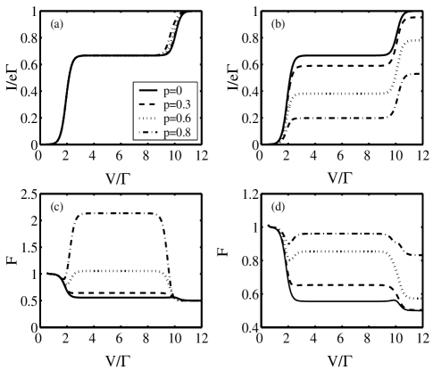
Figure 1: Current (a, b) and Fano factor (c, d) vs. bias-voltage in the P-configuration (a, c) and AP-configuration (b, d) calculated for different polarization $p$ without spin-flip process. Other parameters are: $\epsilon_{d}=1$, $U=4$, and $T=0.1$.

When the leads are in the P-configuration [Fig. 1(a) and (c)], an increase of the polarization will raise the tunneling rates of electrons with the spin-up, $\Gamma_{L\uparrow}$ and $\Gamma_{R\uparrow}$, but reduce the tunneling rates of spin-down electrons, $\Gamma_{L\downarrow}$ and $\Gamma_{R\downarrow}$. Accordingly, this will induce an increase of the spin-up current and a decrease of the spin-down current but it will not affect the total current through the system as shown in Fig. 1(a), because the total current is equal to the summation of the spin-up and spin-down currents. In the case that the Coulomb interaction prevents a double occupancy of the dot, there will be competition between tunneling processes for electrons with up spin and those with down spin. The characteristic times for these two processes are unequal due to polarization: there is fast tunneling for spin-up electrons but slow tunneling for spin-down electrons through the system. The electron spin which tunnel with a lower rate modulates the tunneling of the other spin-direction electron (so-called dynamical spin-blockade).Cottet For a large value of polarization, it leads to an effective bunching of tunneling events and, consequently, to the super-Poissonian shot noise.

It is worth noting that our findings in the P-configuration seem to be in obvious conflict wiht the recent prediction in the sequential tunneling through multi-level systems, in which it was argued that a negative differential conductance (NDC) surely accompanied by the classical super-Poissonian noise.Wacker ; Axel Actually, in these multi-level systems NDC can occur when two levels, separated by nonzero energy difference $\Delta\epsilon=\epsilon_{2}-\epsilon_{1}$, have different coupling strength to the leads. The tunneling through the level which has a stronger coupling to the leads will be suppressed by the Coulomb interaction once the level with weaker coupling is occupied by electron. This reduces the total current, thus induces the NDC. However, this is not the situation in this paper. Here we assume small Zeeman splitting of the level ($\Delta\epsilon=g\mu_{B}B<k_{B}T$) and no energy difference between two spin levels.

Further increasing the bias-voltage above the Coulomb blockade region, i.e, for $eV/2>\epsilon_{d}+U$, opens one more conducting channel and removes spin-blockade. In this region, spin-up and spin-down electrons are tunneling through the different channels and there is no more competition between these two tunneling events. This leads to a reduction of the current fluctuation and the Fano factor becomes the same as in the paramagnetic case.

The situation is completely different in the AP-configuration [Fig. 1(b) and (d)]. An increase of the polarization increases tunneling rates $\Gamma_{L\uparrow}$ and $\Gamma_{R\downarrow}$ and decreases tunneling rates $\Gamma_{L\downarrow}$ and $\Gamma_{R\uparrow}$. An electron with the spin-up, which has tunneled from the left electrode into the QD, remains there for a long time because the tunneling rate $\Gamma_{R\uparrow}$ is reduced by the polarization. This decreases the spin-up current. An increase of the polarization also decreases the spin-down current because it reduces the probability for tunneling of the spin-down electrons into the QD. This will decrease the total current through the system in the Coulomb blockade region, and at the same time increase the shot noise. For large voltage, in the region $eV/2>\epsilon_{d}+U$, both conducting channels become available which results in reduction of the noise comparing with the Coulomb blockade region. In this case the Fano factor does not go to the paramagnetic value because the asymmetry in the tunneling rates are still presented.

Figure 2: Current (a, b) and Fano factor (c, d) in the P-configuration (a, c) and AP-configuration (b, d) calculated for polarization $p=0.5$ and different spin-flip processes. Other parameters are the same as in Fig. 1.

The dependence of Fano factor on the spin-flip scattering with given polarizations $p=0.5$ and $0.9$ can be found from Figs. 2 and 3, respectively. Introducing spin-flip scattering usually results in suppression of the zero-frequency current fluctuation and the Fano factor. This behavior can be easily understood by the following consideration. The spin-flip scattering opens actually one new path for electrons to tunnel out of the QD: a spin-up(down) electron tunneling into the QD can now experience spin-related interaction insider the dot and change its spin-polarization direction and then exit from the QD as a spin-down(up) electron. As a result, an electron which is forced to spend more time in QD due to polarized leads (for example, spin-down electron in the P-configuration and spin-up electron in the AP-configuration) now has greater probability of leaving the dot. In other word, the spin-flip scattering plays a compensating role in tunneling in contrast to that of the lead polarizations and consequently makes an opposite contribution to the current fluctuations. However, this is not true for the P-configuration when double occupation is allowed inside the QD (for $eV/2>\epsilon_{d}+U$). In this region the spin-flip scattering does not have any effect on the Fano factor [Figs. 2(c) and 3(c)]. Spin-up and spin-down electrons are passing through separate channels without changing their spins.

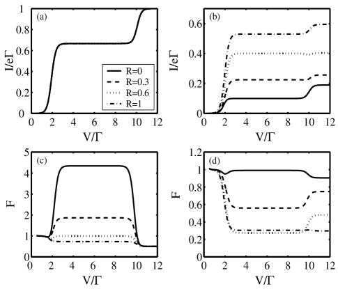
Figure 3: The same as Fig. 2 except for $p=0.9$.

Fig. 4 shows the Fano factor vs. polarization. In the P-configuration, the Fano factor increases with polarization. In AP-configuration, for small spin-flip scattering, Fano factor increases with polarization but for larger $R$ it starts to decrease. This is caused by competition of two effects: increase in the Fano factor due to polarization and, decrease due to spin-flip scattering.

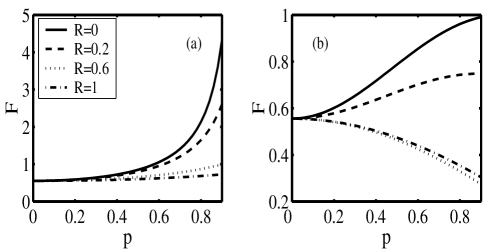
Figure 4: Fano factor vs. polarization $p$ in the P-configuration (a) and the AP-configuration (b) calculated for different spin-flip processes $R$ in the Coulomb blockade region, $V=4$. Other parameters are the same as in Fig. 1

The frequency dependence of the Fano factor in the Coulomb blockade region is given in Fig. 5. For weaker spin-flip scattering, increasing scattering leads to reduction in the Fano factor around zero-frequency, in both configurations [Fig. 5(a) and (c)]. While the larger values of the spin-flip scattering cause different low-frequency behaviors for different leads polarizations [Fig. 5(b) and (d)]. In addition, the strong spin-flip scattering also generates an unambiguous peak in the P-configuration and a hump structure in the AP-configuration approximately located at a nonzero value of frequency $\omega=2R$ (the Rabi frequency), which characterizes the resonant oscillation between two spin states inside the QD. We provide a simple qualitative explanation for this behavior as following: When spin-polarized electrons are injected into the QD from the left lead, the spin Rabi oscillation always allows the electron to escape more easily from the dot to the right polarized lead, thus increasing the deviation of instant current from its average value, which induces enhancement or suppression of shot noise depending on the symmetry of states carrying current.GurvitzIEEE In the P-configuration ($\Gamma_{R\uparrow}>\Gamma_{R\downarrow}$), the outgoing wavefunction of electrons preserve the symmetry with the dominated incoming electrons in the left lead [because we set $\Gamma_{L\uparrow}>\Gamma_{L\downarrow}$ for the polarization leads in this paper, see Eqs. (25) and (26)], which enhances the noise and thus causes a peak in the Fano factor [Fig. 5(a)]. Nevertheless, the situation is complicated for the AP-configuration ($\Gamma_{R\uparrow}<\Gamma_{R\downarrow}$). The anti-symmetry generates a hump structure and finally a dip in the shot noise spectrum for high spin-flip scattering rate [Fig. 5(c)]. Moreover, in the high frequency region, the Fano factor goes to a constant $\frac{1}{2}$ for both configurations.

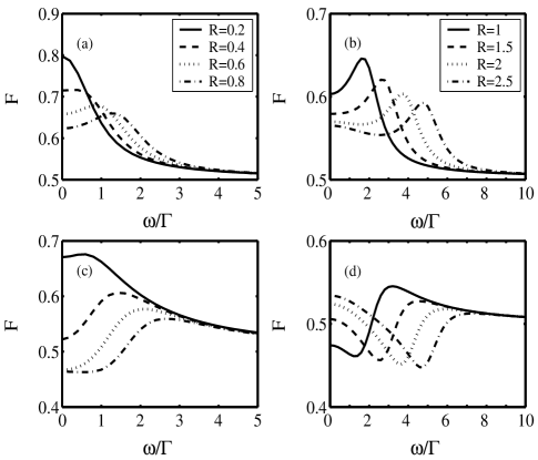
Figure 5: Fano factor in the P-configuration (a, b) and AP-configuration (c, d) vs. frequency calculated in the Coulomb blockade region for different spin-flip processes $R$. Other parameters are: $\epsilon_{d}=1$, $U=4$, $V=3$, $p=0.5$, and $T=0.1$.

III Shot noise in COUPLED QUANTUM DOTS

III.1 Model and quantum rate equations

In this section we consider a resonant tunneling through a CQD with weak coupling between the QDs and the leads. We assume that electron hopping $t$ between the two QDs is also weak. In order to simplify our derivation, we consider here the infinite intradot Coulomb repulsion $U^{\prime}$ and a finite interdot Coulomb interaction $U$, which excludes the state with two electrons in the same QD but two electrons can occupy different QDs. We are again interested in the regime $kT\ll U$, $\Delta$, and $eV\ll\Delta$, so that only one level in each dot contribute to the transport.

The tunneling Hamiltonian for the CQD isDong

$$H = \sum_{\eta,k,\sigma}\epsilon_{\eta k\sigma}c_{\eta k\sigma}^{\dagger}c_{\eta k\sigma}^{{\phantom{\dagger}}}+\epsilon_{1}\sum_{\sigma}c_{1\sigma}^{\dagger}c_{1\sigma}^{{\phantom{\dagger}}}+\epsilon_{2}\sum_{\sigma}c_{2\sigma}^{\dagger}c_{2\sigma}^{{\phantom{\dagger}}}$$ (39)

$$+t\sum_{\sigma}(c_{1\sigma}^{\dagger}c_{2\sigma}^{{\phantom{\dagger}}}+c_{2\sigma}^{\dagger}c_{1\sigma}^{{\phantom{\dagger}}})+U^{\prime}n_{1\uparrow}n_{1\downarrow}+U^{\prime}n_{2\uparrow}n_{2\downarrow}$$

$$+U\sum_{\sigma,\sigma^{\prime}}n_{1\sigma}n_{2\sigma^{\prime}}+\sum_{k,\sigma}(V_{L\sigma}c_{Lk\sigma}^{\dagger}c_{1\sigma}^{{\phantom{\dagger}}}+{\rm{H.c.}})$$

$$+\sum_{k,\sigma}(V_{R\sigma}c_{Rk\sigma}^{\dagger}c_{2\sigma}^{{\phantom{\dagger}}}+{\rm{H.c.}}),$$

where $c_{1(2)\sigma}^{\dagger}$, $c_{1(2)\sigma}$ are creation and annihilation operators for a spin-$\sigma$ electron in the first (second) QD, respectively. $\epsilon_{i}$ ($i=1,2$) is the bare energy level of electrons in the $i$th QD. The other notations are the same as in the SQD case.

Under the assumption of weak coupling between the QDs and the leads, and with the application of the wide band limit in the two leads, electronic transport through this system can be described by the master equation.Dong Here, in order to simplify the analysis, we only consider spin independent tunneling processes and we take the bare mismatch between the two bare levels to be zero ($\epsilon_{1}=\epsilon_{2}=\epsilon_{d}$). The desired quantum rate equations can be readily obtained as:

$$\dot{\rho}_{00} = \Gamma_{L}^{-}\rho_{11}+\Gamma_{R}^{-}\rho_{22}-(\Gamma_{L}^{+}+\Gamma_{R}^{+})\rho_{00},$$ (40a)

$$\dot{\rho}_{11} = \Gamma_{L}^{+}\rho_{00}+\widetilde{\Gamma}_{R}^{-}\rho_{dd}-\Gamma_{L}^{-}\rho_{11}$$ (40d)

$$-\widetilde{\Gamma}_{R}^{+}\rho_{11}+it(\rho_{12}-\rho_{21}),$$

$$\dot{\rho}_{22} = \Gamma_{R}^{+}\rho_{00}+\widetilde{\Gamma}_{L}^{-}\rho_{dd}-\Gamma_{R}^{-}\rho_{22}$$ (40f)

$$-\widetilde{\Gamma}_{L}^{+}\rho_{22}-it(\rho_{12}-\rho_{21}),$$

$$\dot{\rho}_{12} = +it(\rho_{11}-\rho_{22})$$ (40h)

$$-\frac{1}{2}[\Gamma_{L}^{-}+\Gamma_{R}^{-}+\sum_{\eta}\widetilde{\Gamma}_{\eta}^{+}]\rho_{12},$$

$$\dot{\rho}_{dd} = \widetilde{\Gamma}_{R}^{+}\rho_{11}+\widetilde{\Gamma}_{L}^{+}\rho_{22}-(\widetilde{\Gamma}_{L}^{-}+\widetilde{\Gamma}_{R}^{-})\rho_{dd},$$ (40i)

with $\rho_{00}+\rho_{11}+\rho_{22}+\rho_{dd}=1$. Here, $\rho_{00}$ denotes the occupation probability that central region is empty, $\rho_{ii}$ ($i=1,2$) means that the $i$th QD is singly occupied by an electron, and $\rho_{dd}$ stands for the double occupation of the central region (each one of the QDs is occupied by one electron). The non-diagonal elements $\rho_{ij}$ describe the superposition of the two levels in different QDs. The tunneling rates $\Gamma_{\eta}^{\pm}=\Gamma_{\eta}f_{\eta}^{\pm}(\epsilon_{d})$ and $\widetilde{\Gamma}_{\eta}^{\pm}=\Gamma_{\eta}f_{\eta}^{\pm}(\epsilon_{d}+U)$ have the similar prescriptions as in the above section.

The electric current $I_{L}$ flowing from the lead $L$ to the QD can be calculated as:

$$I_{L}/e=\widetilde{\Gamma}_{L}^{-}\rho_{dd}+\Gamma_{L}^{-}\rho_{11}-\widetilde{\Gamma}_{L}^{+}\rho_{22}-\Gamma_{L}^{+}\rho_{00}.$$ (41)

Similarly, for the current flowing from the QD to the $R$ lead we have

$$I_{R}/e=-(\widetilde{\Gamma}_{R}^{-}\rho_{dd}+\Gamma_{R}^{-}\rho_{22}-\widetilde{\Gamma}_{R}^{+}\rho_{11}-\Gamma_{R}^{+}\rho_{00}).$$ (42)

Again, the sign of the current is chosen to be positive when the direction of the current is from the left to the right. It is easy to prove that, in stationary condition, the current conservation is fulfilled $I_{L}=I_{R}$.

III.2 Discussions and calculations of shot noise

In order to calculate the noise power spectrum in CQD, we can simply employ the same procedure that we described in Sec. II. First of all, the simplified quantum rate equations Eq. (40) can be rewritten in the matrix form Eq. (7), in which ${\rho}(t)=(\rho_{00},\rho_{11},\rho_{22},\rho_{dd},\rho_{12},\rho_{21})^{T}$ and the matrix M can be read from Eq. (40). Next, the current operators can be obtained from Eqs. (41) and (42) as follows: $\tilde{\Gamma}_{L}^{-}$ ($\tilde{\Gamma}_{R}^{-}$) describes a tunneling of an electron from the first (second) QD to the $L$$(R)$-lead and it can be considered as a transition rate from $\rho_{dd}$ to $\rho_{22}$ ($\rho_{11}$). Similarly, $\Gamma_{L}^{-}$ ($\Gamma_{R}^{-}$) is a transition rate from $\rho_{11}$ ($\rho_{22}$) to $\rho_{00}$, $\tilde{\Gamma}_{L}^{+}$ ($\tilde{\Gamma}_{R}^{+}$) describes transition from $\rho_{22}$ ($\rho_{11}$) to $\rho_{dd}$, and $\Gamma_{L}^{+}$ ($\Gamma_{R}^{+}$) is a transition rate from $\rho_{00}$ to $\rho_{11}$ ($\rho_{22}$). In the basis $(\rho_{00},\rho_{11},\rho_{22},\rho_{dd},\rho_{12},\rho_{21})^{T}$, the left and right current operators are

$$\hat{\Gamma}_{L}=\left(\begin{array}[]{cccccc}0&\Gamma_{L}^{-}&0&0&0&0\\ -\Gamma_{L}^{+}&0&0&0&0&0\\ 0&0&0&0&0&\tilde{\Gamma}_{L}^{-}\\ 0&0&0&0&0&0\\ 0&0&0&0&0&0\\ 0&0&-\tilde{\Gamma}_{L}^{+}&0&0&0\\ \end{array}\right),$$ (49)

and

$$\hat{\Gamma}_{R}=\left(\begin{array}[]{cccccc}0&0&-\Gamma_{R}^{-}&0&0&0\\ 0&0&0&0&0&-\tilde{\Gamma}_{R}^{-}\\ \Gamma_{R}^{+}&0&0&0&0&0\\ 0&0&0&0&0&0\\ 0&0&0&0&0&0\\ 0&\tilde{\Gamma}_{R}^{+}&0&0&0&0\\ \end{array}\right),$$ (56)

respectively. Finally, we can make corresponding substitution in Eqs. (12), (II.2), and (22) to compute the quantum shot noise in CQD and use Eq. (24) to calculate the Fano factor.

In the following discussions, we set parameters of the CQD under consideration as: $\epsilon_{d}=1$, Coulomb interaction $U=4$, and temperature $T=0.1$. And we also apply the bias voltage $V$ between two leads symmetrically, $eV/2=\mu_{L}=-\mu_{R}$. The zero of energy is chosen to be the Fermi level of the leads in the equilibrium and the energy unit is the one of the tunneling constants.

First, we analyze the zero-frequency shot noise in three limits: (i) zero voltage limit; (ii) the Coulomb blockade region; and (iii) high voltage limit. When the bias voltage is below the resonance, i.e., $eV/2<\epsilon_{d}$, the transport through the system is not energetically allowed and the noise is Poissonian ($F=1$). As the bias voltage is increasing, there occur consecutively two plateaus in the current-voltage characteristic, separated by the thermally broadened step, corresponding to the case of $eV/2>\epsilon_{d}$ (the Coulomb blockade region) and of $eV/2>\epsilon_{d}+U$ (high voltage condition), respectively. On the first plateau, where only one electron can be allowed inside the system, the current $I_{1}$ and the Fano factor $F_{1}$ become:

$$I_{1}=\frac{4t^{2}\Gamma_{R}\Gamma_{L}}{\Gamma_{L}\Gamma_{R}^{2}+4t^{2}\left(2\Gamma_{L}+\Gamma_{R}\right)},$$ (57)

$$F_{1}=1-8\Gamma_{L}\Gamma_{R}t^{2}\frac{3\Gamma_{L}\Gamma_{R}+\Gamma_{R}^{2}+8t^{2}}{\left[4t^{2}\left(2\Gamma_{L}+\Gamma_{R}\right)+\Gamma_{L}\Gamma_{R}^{2}\right]^{2}}.$$ (58)

While in the second plateau, the CQD is in doubly occupied state, and the current $I_{2}$ and the Fano factor $F_{2}$ are:

$$I_{2}=\frac{4t^{2}\Gamma_{R}\Gamma_{L}}{\left(\Gamma_{L}+\Gamma_{R}\right)\left(\Gamma_{L}\Gamma_{R}+4t^{2}\right)},$$ (59)

$$F_{2}=1-8\Gamma_{L}\Gamma_{R}t^{2}\frac{3\Gamma_{L}\Gamma_{R}+\Gamma_{R}^{2}+\Gamma_{L}^{2}+4t^{2}}{\left(\Gamma_{L}+\Gamma_{R}\right)^{2}\left(\Gamma_{L}\Gamma_{R}+4t^{2}\right)^{2}}.$$ (60)

These results are in agreement with the previous derivation from the Laplace transform in Ref. [Brahim, ].

We proceed with numerical calculations. In Fig. 6, we plot the currents and zero-frequency Fano factors in the CQDs as a function of bias voltage for various hopping rates between dots $t/\Gamma=0.2$, $0.5$, $0.7$, and $1.0$. We find that, depending on the relation between the hopping $t$ and the coupling constants $\Gamma_{R(L)}$, the CQD manifests three distinct physical scenarios in its tunneling and low-frequency fluctuation properties: (i) In the case of hopping $2t>\sqrt{\Gamma_{L}\Gamma_{R}}$ ($t>1/2$ in Fig. 7), current increases in the second step ($I_{2}>I_{1}$) and the system exhibits positive differential conductance (PDC). Correspondingly, the Fano factor decreases ($F_{2}<F_{1}$) with increasing bias-voltage; (ii) If the hopping $2t=\sqrt{\Gamma_{L}\Gamma_{R}}$ ($t=1/2$ here), two currents and shot noise are equal to each other, respectively, at the entire region; (iii) While for the hopping $2t<\sqrt{\Gamma_{L}\Gamma_{R}}$ ($t<1/2$ here), current declines in the second step and consequently negative differential conductance (NDC) appears, but the Fano factor raises. Moreover, we find that the Fano factor is always below $1$ in all three regimes, indicating that the quantum shot noise is perpetually smaller than the classical value (sub-Poissonian). Once again, we obtain results differing from those by the recent papers Refs. [Wacker, ; Axel, ]: Our shot noise is enhanced but does not reach super-Poissonian value in the NDC regime.

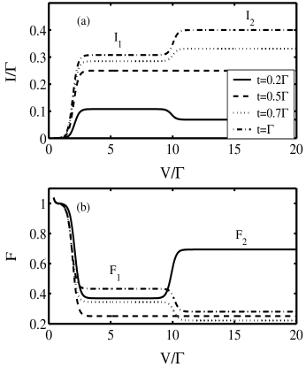
Figure 6: The calculated current (a) and Fano factor (b) vs. bias voltage in the CQDs with different hoppings $t$ between two QDs. Other parameters are: $\Gamma_{L}=\Gamma_{R}=\Gamma$, $\epsilon_{d}=1$, $U=4$, and $T=0.1$.

Fig. 7 and 8 shows the current and the Fano factor as a function of the tunneling constants $\Gamma_{R}$ and $\Gamma_{L}$ in the current plateaus regions. For small hopping $t<\Gamma_{L}$ the currents $I_{1}$ and $I_{2}$ show non-monotonic behavior with increasing $\Gamma_{R}$ [Fig. 7(a)]: They increase for small couplings and, decrease when couplings are larger. With increasing $\Gamma_{L}$ [Fig. 7(b)], $I_{1}$ increases for small couplings and gradually saturates. On the contrary, $I_{2}$ shows an analogous non-monotonic behavior as in Fig. 7(a). The NDC appears whenever $I_{2}$ becomes smaller than $I_{1}$ and it is most pronounced for larger coupling to the left lead $\Gamma_{L}\gg\Gamma_{R}$. In small hopping limit ($t\ll\Gamma_{L(R)}$), Eqs. (57) and (59) can be simplified, respectively, to:

$$I_{1}=\frac{4t^{2}}{\Gamma_{R}}=\frac{4t^{2}}{\Gamma_{d_{1}}},$$ (61)

and

$$I_{2}=\frac{4t^{2}}{\Gamma_{R}+\Gamma_{L}}=\frac{4t^{2}}{\Gamma_{d_{2}}},$$ (62)

where $\Gamma_{d_{1}}=\Gamma_{R}$ and $\Gamma_{d_{2}}=\Gamma_{R}+\Gamma_{L}$ are the decoherence rates due to the interaction with the leads. Actually, if we simplify Eq. (40h) in the regions of the first and second current plateaus, we obtain:

$$\dot{\rho}_{12}=it(\rho_{11}-\rho_{22})-\frac{1}{2}\Gamma_{d_{1}}\rho_{12},$$ (63)

and

$$\dot{\rho}_{12}=it(\rho_{11}-\rho_{22})-\frac{1}{2}\Gamma_{d_{2}}\rho_{12},$$ (64)

respectively. It is clear that the two rates indeed characterize the decay of coherent superposition. Conservation of current allows us to express the current through the system as $I=it(\rho_{12}-\rho_{21})$. From Eqs. (63) and (64) one can see that for large decoherence rates, $\Gamma_{d_{1(2)}}\gg t$, the probability of tunneling between the two dots, $\rho_{12}$, becomes purely damped with time, implying the destructive quantum interference between the coherent superposition of two quantum dot states and the electronic state in the continuum (right lead) in the process of tunneling,Gur which induces localization of the electron in the first dot (QDs form ionic-like bonds), as well as the reduction of the two resonant currents $I_{1}$ and $I_{2}$.

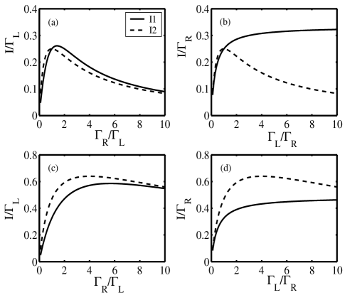
Figure 7: Current vs. bias-voltage in the CQDs calculated for different coupling constants $\Gamma_{R}$ (a, c) and $\Gamma_{L}$ (b, d). Other parameters are: $U=4$, $\epsilon_{d}=1$, $T=0.1$, $t=0.5$ (a, b) and $t=2$ (c, d).

In the case of high voltage, the presence of one excess electron inside the dots further destroys coherent superposition because there is no possibility of electron tunneling between the two dots due to the infinite intradot Coulomb interaction. The decoherence rate in this case is a sum of the two rates: $\Gamma_{L}$, which describes the tunneling of the second electron inside the system and $\Gamma_{R}$, which stands for the tunneling of an electron to the right lead. The decrease of the current $I_{2}$ is caused by both of these processes [Figs. 7(a) and (b)], therefore it is smaller that $I_{1}$ and NDC appears. In the NDC regime the noise increases but it remains sub-Poissonian (Fig. 8).

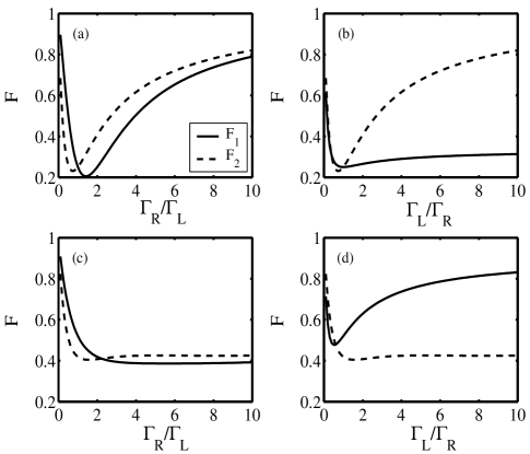
Figure 8: Fano factor vs. bias-voltage in the CQDs calculated for different coupling constants $\Gamma_{L}$ (a, c) and $\Gamma_{R}$ (b, d). Other parameters are as in Fig. 7

In the large hopping limit ($t\gg\Gamma_{d_{1(2)}}$), an electron can shuttle between the two dots many times in a phase-coherent way before it tunnels out into the right lead and thus becomes delocalized (covalent-like bonds). In this limit, the current and the Fano factor approach to the single QD values Eqs. (32)–(35).

The Fano factor is plotted against normalized frequency in Fig. 9. Similar noise properties are found for a coherently coupled double well structure.Sun In the Coulomb blockade regime [Fig. 9], if an electron from the left lead is injected into the first QD, no further electrons can enter in the QD until this electron is removed. The time scale for this removal process is determined by $t^{-1}$. Thus, in small hopping limit, the zero-frequency shot noise is reduced with increasing $t$ due to the interdot Coulomb blockade effect [Fig. 9(a)]. As the frequency increases, the electron inside the first QD has more opportunity to instantly tunnel into the second QD, which enhances the shot noise. While for the high values of hopping, the electron in the second QD can either escape to the right lead, which takes place on a time scale determined by $\Gamma_{R}^{-1}$, or, it can periodically return to the first QD at a frequency $2t$ (the Rabi frequency). If $2t\gg\Gamma_{R}$, there is larger probability for the electron in the second QD to tunnel back into the first QD than to escape to the right lead, which prevent another electron from entering the first QD. Thus at large values of $t$ noise suppression occurs at $\omega=2t$, the dip in the Fano factor [Figs. 9(b)].

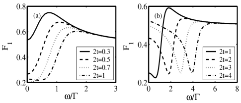
Figure 9: Fano factor vs. frequency calculated in the Coulomb blockade regime for different hoppings $t$ between the QDs. Other parameters are: $\Gamma_{R}=\Gamma_{L}=\Gamma$, $V=6$, $\epsilon_{d}=1$, $U=4$, and $T=0.1$.

The influences of the coupling constants on the frequency-dependent noise characteristic is given in Fig. 10. When only one electron is present inside the CQD system [Figs. 10(a) and (b)], decreasing coupling to the right lead (decreasing decoherence rate) leads to the noise enhancement in the low frequency region. On the other hand, the decreasing decoherence rate results in the transformation of the electronic states in the CQD from the ionic-like bond to the covalent-like bond and the formation of a dip in the shot noise spectrum at moderately high frequency $\omega=2t$. In the large voltage region, when doubly occupancy is allowed, the decoherence rate is given as a sum of $\Gamma_{L}$ and $\Gamma_{R}$ and both coupling constants influence shot noise in the same way [Figs. 10(c) and (d)].

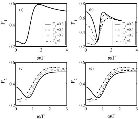
Figure 10: Fano factor vs. frequency calculated in the Coulomb blockade regime (a, b) and in the large voltage region (c, d) for different coupling constants $\Gamma_{L}$ and $\Gamma_{R}$ between the QDs and the leads. Other parameters are: $t=0.5$, $\Gamma_{R}=\Gamma$ (a, c), $\Gamma_{L}=\Gamma$ (b, d) $V=6$ (a, b), $V=12$ (c, d), $\epsilon_{d}=1$, $U=4$, and $T=0.1$.

IV CONCLUSION

In this paper we have presented theoretical investigations of the shot noise spectrum in resonant tunneling through a interacting quantum coupled system, in which quantum interference effects play an important role in its transport and fluctuation properties. For this purpose, we have modified the well-known generation-recombination approach, which has been established for over ten years to study the shot noise in single-electron tunneling devices based on the classical rate equations, to incorporate with the quantum version of rate equations. We have also developed a convenient numerical technique to compute the shot noise by applying the matrix spectral decomposition.

As applications of our formalism, we have systematically analyzed the current shot noise, as functions of bias-voltage and frequency, through (i) a single QD connected to two ferromagnetic leads with weak intradot spin-flip scattering, and (ii) coherently coupled QDs. The influence of the Coulomb interaction and coherent electron evolution on the Fano factor has been investigated in detail. First we have given some analytic expressions for the zero-frequency Fano factors in two special cases: Coulomb blockade regime and double occupation region (high bias-voltage limit). It is shown that these results are in perfect agreement with previous analysis in the literature.

In addition, we have performed numerical simulations for the two systems. For the single QD, we found that: 1) In the Coulomb blockade regime, an increase of the polarization leads to an enhancement of the zero-frequency current noise in both configurations, even a super-Poissonian value in the P-configuration due to dynamical spin-blockade, implying bunching effect in tunneling processes. For the AP-configuration, this enhancement results from the asymmetry in the tunneling rates into and out of the QD ($\Gamma_{L\uparrow}>\Gamma_{R\uparrow}$ but $\Gamma_{L\downarrow}<\Gamma_{R\downarrow}$) for each spin separately; 2) The spin-flip scattering compensates for polarization of the leads (removing the dynamical spin-blockade) and causes reduction of the current fluctuation and Fano factor; 3) The frequency-dependent Fano factors clearly show a peak in the P-configuration but a dip in the AP-configuration at the Rabi frequency $\omega=2R$, reflecting differing symmetries of states carrying current. For the CQD, we have predicted that depending on the relation between the hopping $t$ and the dot-leads couplings $\Gamma_{L(R)}$, there are three distinct physical scenarios in its tunneling and low-frequency fluctuation properties. More importantly, we found appearance of NDC in the current-voltage characteristic and corresponding enhancement of the Fano factor but still remaining sub-Poissonian in the case of $t<\sqrt{\Gamma_{L}\Gamma_{R}}$. Our sequent qualitative analysis claimed that this feature is a result of the enhanced decoherence rate induced by the presence of the second electron inside the system [Eqs. (61) and (62)]. Moreover, the destructive interference between two QDs states leads to a dip in the frequency-related Fano factor at the Rabi frequency $2t$, which is also controlled by the tunnel coupling $\Gamma_{R}$ to the right lead in the Coulomb blockade regime.

Expectably, our results show that shot noise measurements can provide more useful information about quantum coherence of electron wavefunction than do conventional transport measurements.

- (1) For an overview of quantum shot noise, please refer to Ya.M. Blanter and M. Büttiker, Phys. Rep. 336, 1 (2000).
- (2) C. Beenakker and C. Schönenberger, Phys. Today, May 2003, 37 (2003).
- (3) For a review, see W.G. van der Wiel, S.De Franceschi, J.M. Elzerman, T. Fujisawa, S. Tarucha, L.P. Kouwenhoven, Rev. Mod. Phys. 75, 1 (2003).
- (4) S.A. Gurvitz, Phys. Rev. B 56, 15215 (1997).
- (5) H.B. Sun and G.J. Milburn, Phys. Rev. B 59, 10748 (1999).
- (6) B. Elattari and S.A. Gurvitz, Phys. Lett. A 292, 289-294 (2002).
- (7) D. Mozyrsky, L. Fedichkin, S.A. Gurvitz, and G.P. Berman, Phys. Rev. B 66, 161313 (2002).
- (8) S.A. Gurvitz, L. Fedichkin, D. Mozyrsky, and G.P. Berman, Phys. Rev. Lett 91, 66801 (2003).
- (9) R. Aguado and T. Brandes, Phys. Rev. Lett. 92, 206601 (2004).
- (10) H.A. Engel and D. Loss, Phys. Rev. Lett. 93, 136602 (2004).
- (11) S.A. Gurvitz, cond-mat/0406010 (2004).
- (12) Yu.V. Nazarov, Physica B 189, 57 (1993).
- (13) S.A. Gurvitz and Ya.S. Prager, Phys. Rev. B 53, 15932 (1996).
- (14) Bing Dong, H.L. Cui, and X.L. Lei, Phys. Rev. B 69 35324 (2004).
- (15) S. Hershfield, J.H. Davies, P. Hyldgaard, C.J. Stanton and J.W. Wilkins, Phys. Rev. B 47, 1967 (1993).
- (16) A.N. Korotkov, Phys.Rev. B 49, 10381 (1994).
- (17) U. Hanke, Yu.M. Galperin, K.A. Chao and Nanzhi Zou, Phys. Rev. B 48, 17209 (1993)
- (18) S.I. Erlingsson, Yu.V. Nazarov, Phys. Rev. B 66, 155327 (2002).
- (19) J.H. Davies, P. Hyldgaard, S. Hershfield, and J.W. Wilkins, Phys. Rev. B 46, 9620 (1992).
- (20) A. Cottet and W. Belzig, Europhys. Lett. 66 405 (2004); A. Cottet, W. Belzig, and C. Bruder, Phys. Rev. Lett. 92, 206801 (2004); A. Cottet, W. Belzig, and C. Bruder, Phys. Rev. B 70, 115315 (2004).
- (21) A. Thielmann, M.H. Hettler, J. König, and G. Schön, cond-mat/0406647 (2004).
- (22) G. Kießlich, A. Wacker, and E. Schöll, Phys. Rev. B 68, 125320 (2003).
- (23) S.A. Gurvitz, Phys. Rev. B 57, 6602 (1998).