Spin-1/2 fermions: crossover from weak to strong attractive interaction

K. Ziegler
Institut fΓΌr Physik, UniversitΓ€t Augsburg, Germany
e-mail: ziegler@physik.uni-augsburg.de

Abstract:

The formation and dissociation of bosonic molecules in an optical lattice, formed by spin-1/2 fermionic atoms, is considered in the presence of an attractive nearest-neighbor interaction. A mean-field approximation reveals three different phases at zero temperature: an empty, a condensate and a Mott-insulating phase. The density of fermionic atoms and the density of bosonic molecules indicate a characteristic behavior with respect to the interaction strength that distinguishes between a dilute and a dense regime. In particular, the attractive interaction favors the formation of molecules in the dilute regime and the dissociation of atoms in the dense regime.

1 Introduction

Feshbach resonances provide a powerful tool to vary the interaction strength of atomic gases [1]. Physical effects, like the formation of molecules, Bose-Einstein condensation or Cooper pairing in fermionic systems depend strongly on the strength of the interparticle interaction [2, 3, 4, 5, 6]. A model for spin-1/2 fermions with attractive nearest-neighbor interaction is studied to describe the formation and dissociation of bosonic molecules in a grand-canonical gas of fermionic atoms. The model depends on three tunable parameters, the fermionic tunneling rate ${\bar{t}}$, the fugacity $\zeta$ of the grand-canonical gas, and the molecular tunneling rate $J$. $J$ also controls the attractive nearest-neighbor interaction of the model.

A difference in comparison with previous works [8, 9, 10, 11] is that we study the $T=0$ properties of a Fermi gas in an optical lattice. A consequence of the latter is that a Mott-insulating state can be identified, whereas $T=0$ avoids thermal fluctuations of the system. In this case a mean-field approximation should give reasonable results, provided that quantum fluctuation are not too strong.

A qualitative picture of the $T=0$ phase diagram can be given by an estimate of the energies. There is a single-particle potential due to the chemical potential of the fermionic atoms. It is assumed that the chemical potential of the molecules is the same as that of the constituting fermionic atoms, i.e. the effective chemical potential of a molecule is twice as that of a single fermionic atom. If this potential is sufficiently negative the optical lattice is empty, since particles cannot overcome the potential barrier. The kinetic energy, however, represented by the tunneling rates ${\bar{t}}$ and $J$, competes with the chemical potential and favors the creation of a Fermi gas and/or a molecular Bose gas. The interaction plays a crucial role in this regime: In addition to the formation of (local) bosonic molecules, the attractive interaction between the fermionic atoms may lead to the formation of Cooper pairs, which can be considered as β€œnon-local molecules”. For sufficiently large chemical potential the optical lattice will be filled with two atoms per lattice site, which is a Mott-insulating state. This Mott state differs from the Mott insulator of a half-filled Fermi lattice gas with repulsive interaction (Hubbard model [14]), where the interaction creates a ground state with one fermion per lattice site. In other words, the Mott insulator in the system with attractive interaction is a special kind of insulator that is created by the Pauli exclusion, and not by a finite repulsive interaction, in contrast to the Hubbard model at half filling.

A mean-field theory is applied to discuss a Mott insulator and a condensed phase. Depending on the tunable parameters of the model, the density of dissociated atoms and the density of molecules in the condensed phase are investigated. It will be shown that the density of dissociated atoms increases with the total number of particles, reaches a maximum and decreases, whereas the density of molecules is a monotoneously increasing function.

2 Model: Hamiltonian and Functional Integral

A gas of spin-1/2 fermions in an optical lattice is considered. Using fermionic creation (annihilation) operators cr​σ†subscriptsuperscriptπ‘β€ π‘ŸπœŽc^{\dagger}_{r\sigma} ($c_{r\sigma}$) for spin $\sigma$ and at site $r$ (a minimum in the optical lattice), the Hamiltonian of the Fermi gas is

H=βˆ’tΒ―β€‹βˆ‘<r,rβ€²>βˆ‘Οƒ=↑,↓cr​σ†​crβ€²β€‹Οƒβˆ’Jβ€‹βˆ‘<r,rβ€²>cr↑†​cr′↑​cr↓†​crβ€²β†“βˆ’ΞΌβ€‹βˆ‘rβˆ‘Οƒ=↑,↓cr​σ†​cr​σ.𝐻¯𝑑subscriptabsentπ‘Ÿsuperscriptπ‘Ÿβ€²absentsubscriptπœŽβ†‘β†“subscriptsuperscriptπ‘β€ π‘ŸπœŽsubscript𝑐superscriptπ‘Ÿβ€²πœŽπ½subscriptabsentπ‘Ÿsuperscriptπ‘Ÿβ€²absentsubscriptsuperscriptπ‘β€ β†‘π‘Ÿabsentsubscript𝑐↑superscriptπ‘Ÿβ€²absentsubscriptsuperscriptπ‘β€ β†“π‘Ÿabsentsubscript𝑐↓superscriptπ‘Ÿβ€²absentπœ‡subscriptπ‘ŸsubscriptπœŽβ†‘β†“subscriptsuperscriptπ‘β€ π‘ŸπœŽsubscriptπ‘π‘ŸπœŽH=-{\bar{t}}\sum_{<r,r^{\prime}>}\sum_{\sigma=\uparrow,\downarrow}c^{\dagger}_{r\sigma}c_{r^{\prime}\sigma}-J\sum_{<r,r^{\prime}>}c^{\dagger}_{r\uparrow}c_{r^{\prime}\uparrow}c^{\dagger}_{r\downarrow}c_{r^{\prime}\downarrow}-\mu\sum_{r}\sum_{\sigma=\uparrow,\downarrow}c^{\dagger}_{r\sigma}c_{r\sigma}. (1)

$<r,r^{\prime}>$ refers to nearest-neighbor sites $r$ and $r^{\prime}$. A chemical potential term for molecules

βˆ’Ξ½β€‹βˆ‘rcr↑†​cr↑​cr↓†​crβ†“πœˆsubscriptπ‘Ÿsubscriptsuperscriptπ‘β€ β†‘π‘Ÿabsentsubscriptπ‘β†‘π‘Ÿabsentsubscriptsuperscriptπ‘β€ β†“π‘Ÿabsentsubscriptπ‘β†“π‘Ÿabsent-\nu\sum_{r}c^{\dagger}_{r\uparrow}c_{r\uparrow}c^{\dagger}_{r\downarrow}c_{r\downarrow}

has been neglected because it leads only to a shift of $J$ in terms of the subsequent mean-field calculation. Similar Hamiltonians were considered in a number of papers [8, 9, 10]. The first term describes tunneling of individual fermions in the optical lattice with rate ${\bar{t}}$, the second term tunneling of local fermion pairs (i.e. bosonic molecules) between nearest-neighbor sites with rate $J$. It should be noticed that the latter is also responsible for an attractive interaction between fermions with different spin ($J>0$). However, there is no local (diagonal) interaction, all the fermionic interaction is carried by the nearest-neighbor term. The bosonic molecules experience a local repulsive (hard-core) interaction, since their constituent atoms are fermions and obey the Pauli exclusion. For the limiting case ${\bar{t}}=0$ only bosonic molecules can appear, for $J=0$ only non-interacting fermionic atoms. The chemical potential $\mu$ controls the number of particles in a grand-canonical ensemble. The latter is given by the partition function

$$Z=Tre^{-\beta H}.$$

Space-time correlations of fermions are described by the Green’s function

$$G_{r,t,\sigma;r^{\prime},0,\sigma^{\prime}}={1\over Z}Tr\Big{[}e^{-(\beta-t)H}c_{r,\sigma}e^{-tH}c^{\dagger}_{r^{\prime},\sigma^{\prime}}\Big{]}.$$

The partition function can also be written in terms of a Grassmann integral [13, 15] as

$$Z=\int e^{-S}{\cal D}[\psi],$$

where the action $S$ for spin-1/2 fermions with attractive interaction, related to the Hamiltonian in Eq. (1), reads

$$S=\sum_{x}(\psi_{x,1}{\bar{\psi}}_{x,1}+\psi_{x,2}{\bar{\psi}}_{x,2})-\sum_{r,r^{\prime},t}(\zeta\delta_{r,r^{\prime}}+{\bar{t}}w_{r,r^{\prime}})(\psi_{r,t,1}{\bar{\psi}}_{r^{\prime},t+1,1}+\psi_{r,t,2}{\bar{\psi}}_{r^{\prime},t+1,2})$$
$$-J\sum_{r,r^{\prime},t}\psi_{r,t,1}{\bar{\psi}}_{r^{\prime},t+1,1}\psi_{r,t,2}{\bar{\psi}}_{r^{\prime},t+1,2}$$ (2)

with space-time coordinates $x=(r,t)$. $w_{r,r^{\prime}}$ is $1/2d$ for nearest-neighbor sites on a $d$-dimensional cubic optical lattice and zero otherwise, and $\zeta=e^{\mu}$ is the fugacity. The Green’s function then reads

$$G_{x,\sigma;x^{\prime},\sigma^{\prime}}=\langle\psi_{x,\sigma}{\bar{\psi}}_{x^{\prime},\sigma^{\prime}}\rangle\equiv\int\psi_{x,\sigma}{\bar{\psi}}_{x^{\prime},\sigma^{\prime}}e^{-S}{\cal D}[\psi]/Z.$$

After renaming ${\bar{\psi}}$ by a time shift $t\to t-1$

$${\bar{\psi}}_{r,t,j}\to{\bar{\psi}}_{r,t-1,j}\ \ \ (j=1,2)$$ (3)

the action reads

$$S^{\prime}=\sum_{x}(\psi_{x,1}\partial_{t}^{T}{\bar{\psi}}_{x,1}+\psi_{x,2}\partial_{t}^{T}{\bar{\psi}}_{x,2})-\sum_{r,r^{\prime},t}(\zeta\delta_{r,r^{\prime}}+{\bar{t}}w_{r,r^{\prime}})(\psi_{r,t,1}{\bar{\psi}}_{r^{\prime},t,1}+\psi_{r,t,2}{\bar{\psi}}_{r^{\prime},t,2})$$
$$-J\sum_{r,r^{\prime},t}\psi_{r,t,1}{\bar{\psi}}_{r^{\prime},t,1}\psi_{r,t,2}{\bar{\psi}}_{r^{\prime},t,2}.$$

The quartic interaction term is now diagonal with respect to time. It can be decoupled by two complex Hubbard-Stratonovich fields $\phi_{x}$, $\chi_{x}$ [15]. The linear combination $i\phi+\chi$ couples to fermions like

$$(i\phi_{x}+\chi_{x})\psi_{x,1}\psi_{x,2}+h.c..$$ (4)

This coupling is similar to the atom-molecule coupling discussed in Refs. [11, 12]. There is a difference, however, by the fact that we started from the fermionic model and derived an effective electron-boson model, whereas the other authors started from an electron-boson model and derived the effective fermion model. In both cases an effective coupling constants can be evaluated from the original model, an effective fermion-fermion coupling in Ref. [11] and an effective fermion-boson coupling in our model. Although this is an interesting problem it will not be pursued in this paper. Instead, the fermions are integrated out in $Z$, since they appear only in a quadratic form in the action. This step provides an effective model only for bosons: the integration gives a fermion determinant and the resulting fuctional $Z$ depends only on the complex fields $\phi$ and $\chi$ with the effective action

$$S_{eff}=(\phi,v^{-1}\phi)+{1\over 2J}(\chi,\chi)-{1\over 2}\log(\det A)$$ (5)

with the antisymmetric space-time matrix

$$A=\pmatrix{0&i\phi+\chi&\zeta+{\bar{t}}w-\partial_{t}^{T}&0\cr-i\phi-\chi&0&0&\zeta+{\bar{t}}w-\partial_{t}^{T}\cr-\zeta-{\bar{t}}w+\partial_{t}&0&0&i{\bar{\phi}}+{\bar{\chi}}\cr 0&-\zeta-{\bar{t}}w+\partial_{t}&-i{\bar{\phi}}-{\bar{\chi}}&0\cr}$$

with $v^{-1}=(w+2{\bf 1})^{-1}/J$.

$\phi$ corresponds to the conventional BCS field in the case of a local interaction. The additional field $\chi$ is necessary for the nearest-neighbor interaction to ensure that the Hubbard-Stratonovich decoupling is well-defined [15]. It will be discussed subsequently that the mean-field approximation yields a linear relationship between these two fields.

2.1 Atomic and Molecular Densities

The densities of atoms and molecules can be measured as expectation values of the Grassmann fields. For this purpose the original fields are used, i.e., the fields before the time shift in Eq. (3), to write

$$\langle...\rangle=\int...e^{-S}{\cal D}[\psi]/Z.$$

The action $S$ of Eq. (2) can be expanded in $Z$ around

$$S_{0}=\sum_{x}(\psi_{x,1}{\bar{\psi}}_{x,1}+\psi_{x,2}{\bar{\psi}}_{x,2})$$

to obtain

$$Z=\sum_{l\geq 0}{1\over l!}\int e^{-S_{0}}(S_{0}-S)^{l}{\cal D}[\psi].$$

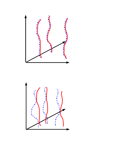
This expansion can be viewed as an expansion in terms of world lines in a space-time lattice. There are two types of world lines, individual fermion lines with spin $\sigma$ and molecular world lines, as shown in Fig. 1. For a given point in space and time $x$ the contribution from the polynomial $(S_{0}-S)^{l}$ is either a factor 1 (i.e. no contribution from $(S_{0}-S)^{l}$ at this point), a factor $\psi_{x,\sigma}{\bar{\psi}}_{x,\sigma}$, or a factor $\psi_{x,1}{\bar{\psi}}_{x,1}\psi_{x,2}{\bar{\psi}}_{x,2}$. To measure the probability of the appearence of these factors in $Z$, an expectation value with respect to the Grassmann field can be introduced. In particular, the density of dissociated atoms reads

$$n_{f,x}=-\langle\psi_{x,1}{\bar{\psi}}_{x,1}+\psi_{x,2}{\bar{\psi}}_{x,2}+2\psi_{x,1}{\bar{\psi}}_{x,1}\psi_{x,2}{\bar{\psi}}_{x,2}\rangle$$

and the density of molecules

$$n_{m,x}=\langle 1+\psi_{x,1}{\bar{\psi}}_{x,1}+\psi_{x,2}{\bar{\psi}}_{x,2}+\psi_{x,1}{\bar{\psi}}_{x,1}\psi_{x,2}{\bar{\psi}}_{x,2}\rangle.$$

The truncated expectation value

$$C_{12}=\langle\psi_{x,1}{\bar{\psi}}_{x,1}\psi_{x,2}{\bar{\psi}}_{x,2}\rangle-\langle\psi_{x,1}{\bar{\psi}}_{x,1}\rangle\langle\psi_{x,2}{\bar{\psi}}_{x,2}\rangle$$

gives

$$n_{f,x}=-\langle 1+\psi_{x,1}{\bar{\psi}}_{x,1}\rangle\langle\psi_{x,2}{\bar{\psi}}_{x,2}\rangle-\langle 1+\psi_{x,2}{\bar{\psi}}_{x,2}\rangle\langle\psi_{x,1}{\bar{\psi}}_{x,1}\rangle-2C_{12}$$ (6)

and

$$n_{m,x}=\langle 1+\psi_{x,1}{\bar{\psi}}_{x,1}\rangle\langle 1+\psi_{x,2}{\bar{\psi}}_{x,2}\rangle+C_{12}.$$ (7)

It will be seen below that $C_{12}$ vanishes in mean-field approximation.

In the Mott-insulating phase a fully occupied lattice is expected, i.e., two fermionic atoms (= one molecule) per site, as the only commensurate state, since there is no repulsive interaction which could maintain a commensurate state. Any other groundstate of the system is a condensate, except for the empty lattice. The remaining question is how the condensate varies with the total number of atoms and molecules in the system. It is obvious that the total density of particles increases monotoneously with the fugacity. However, it is less clear how the formation of molecules or the dissociation of atoms is affected by an increasing fugacity. Moreover, a naive picture suggests that the density of molecules increases monotoneously with an increasing attractive coupling of the fermionic atoms $J$. It will be shown in terms of a mean-field approximation that this is not the case.

3 The Saddle-point Equation

The saddle-point condition for the effective action in Eq. (5) is

$$\delta S_{eff}=0.$$ (8)

This gives a nonlinear difference equation. A simple ansatz for its solution is given by uniform fields $\phi$ and $\chi$ (mean-field approximation). Then Eq. (8) reads

$$\cases{\phi=3JG(\phi-i\chi)\cr\chi=-i2JG(\phi-i\chi)\cr}$$ (9)

with the integral

$$G=\int_{-1}^{1}{\rho(x)\over\sqrt{(-i\chi+\phi)^{2}({-i\bar{\chi}}+{\bar{\phi}})^{2}+2(s^{2}+1)(-i\chi+\phi)(-i{\bar{\chi}}+{\bar{\phi}})+(s^{2}-1)^{2}}}dx$$ (10)

and s=ΞΆ+t¯​xπ‘ πœΒ―π‘‘π‘₯s=\zeta+{\bar{t}}x. $\rho(x)$ is the density of states for the nearest-neighbor tunneling term $w$.

There is a trivial solution $\phi=\chi=0$ and a nontrivial solution

$$G=1/J,\ \ \ \chi=-2i\phi/3.$$ (11)

This is the same mean-field equation as in the BCS theory, if $J$ is considered as the coupling constant of the fermions.

The solution in Eq. (11) implies a non-negative value for

$$(-i\chi+\phi)(-i{\bar{\chi}}+{\bar{\phi}})=\phi{\bar{\phi}}/9\equiv|\phi|^{2}/9.$$

Then $G$ in Eq. (10) reads

$$G=\int_{-1}^{1}{\rho(x)\over\sqrt{|\phi|^{4}/81+2(s^{2}+1)|\phi|^{2}/9+(s^{2}-1)^{2}}}dx$$ (12)

which descreases monotoneously with $|\phi|^{2}$. If $(s^{2}-1)^{2}$ becomes 0 inside the interval of integration $-1\leq x\leq 1$ the integral diverges for $|\phi|\to 0$. Therefore, there is a non-zero solution of $\phi$ for any value of $J>0$. On the other hand, if $(s^{2}-1)^{2}$ does not become 0 inside the interval of integration, there is a non-zero solution only for sufficiently large values of $J$ (cf. Fig. 2).

The densities can be evaluated within the saddle-point approximation. A straightforward calculation gives for the expectation values, used in $n_{f,x}$ and $n_{m,x}$, the expression

$$\langle\psi_{x,j}{\bar{\psi}}_{x,j}\rangle=-{1\over 2}+{1\over 2}\int_{-1}^{1}{|\phi|^{2}/9+s^{2}-1\over\sqrt{|\phi|^{2}/81+2(s^{2}+1)|\phi|^{2}/9+(s^{2}-1)^{2}}}\rho(x)dx$$ (13)

and

⟨ψx,jβ€‹ΟˆΒ―x,jβ€²βŸ©=0(jβ‰ jβ€²).delimited-⟨⟩subscriptπœ“π‘₯𝑗subscriptΒ―πœ“π‘₯superscript𝑗′0𝑗superscript𝑗′\langle\psi_{x,j}{\bar{\psi}}_{x,j^{\prime}}\rangle=0\ \ \ (j\neq j^{\prime}).

4 Results

Using the mean-field approximation of the previous section the following quantities are evaluated: the order parameter $|\phi|^{2}$ of the condensate, the $T=0$ phase diagram, and $n_{f}(|\phi|^{2},\zeta)$, $n_{m}(|\phi|^{2},\zeta)$.

4.1 $\phi=0$

In the case of a vanishing order parameter (i.e. $\phi=0$) only independent fermions are described by the mean-field approach. Then the diagonal element in Eq. (13) is

$$\langle\psi_{x,j}{\bar{\psi}}_{x,j}\rangle=-\int_{-1}^{1}\Theta(1-(\zeta+tx)^{2})\rho(x)dx.$$

If $s^{2}<1$ for the entire interval of integration, i.e.,

$$-1+{\bar{t}}<\zeta<1-{\bar{t}}$$

both densities vanish: $n_{f}=n_{m}=0$. On the other hand, if $s^{2}>1$ for the entire interval of integration, i.e.,

$$\zeta>1+{\bar{t}}$$

one obtains $n_{f}=0$, $n_{m}=1$. Thus all lattice sites are occupied by bosonic molecules. There is also an intermediate regime for $1-{\bar{t}}<\zeta<1+{\bar{t}}$ where nf,nmβ‰ 0subscript𝑛𝑓subscriptπ‘›π‘š0n_{f},n_{m}\neq 0. Details of this behavior are shown in Figs. 2 and 3.

4.2 Ο•β‰ 0italic-Ο•0\phi\neq 0

For the beginning the special case ${\bar{t}}=0$ (molecules cannot dissociate) is considered. Then the integrand in Eq. (13) is constant with respect to the integration variable $x$ and yields

$$\langle\psi_{x,j}{\bar{\psi}}_{x,j}\rangle=-1/2+{1\over 2}{|\phi|^{2}/9+\zeta^{2}-1\over\sqrt{|\phi|^{4}/81+2(\zeta^{2}+1)|\phi|^{2}/9+(\zeta^{2}-1)^{2}}}.$$

The saddle-point solution

$$|\phi|^{2}=9(\sqrt{4\zeta^{2}+J^{2}}-1-\zeta^{2})$$

exists for

$$\cases{\sqrt{1-J}<\zeta<\sqrt{1+J}&if $0<J\leq 1$\cr 0<\zeta<\sqrt{1+J}&if $J>1$\cr}.$$

The corresponding phase diagram is shown in Fig. 4. This result yields

$$\langle\psi_{x,j}{\bar{\psi}}_{x,j}\rangle=-1/2-1/J+\sqrt{\zeta^{2}/J^{2}+1/4}.$$

In the general case with dissociated atoms (i.e. for ${\bar{t}}>0$), the density of states in $G$ can be approximated by a constant as $\rho(x)=1/2$. Moreover, for small $J$ the integral in Eq. (12) can be easily performed, giving the saddle-point solution of the order parameter
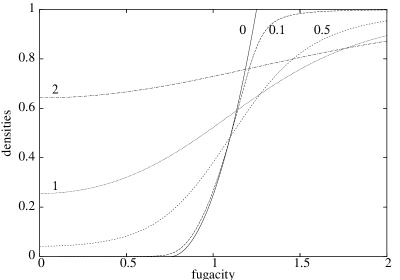
$$|\phi|^{2}\sim 4{\bar{t}}^{2}e^{-4{\bar{t}}/J}\ \ \ \ (1-{\bar{t}}<\zeta<1+{\bar{t}}).$$

The model parameters $\zeta$, $J$, and ${\bar{t}}$ control the densities. However, in a realistic situation the order parameter $\phi$ and the densities $n_{f},n_{m}$ will be measured. Therefore, the densities for a given value of $|\phi|$ are plotted as functions of the fugacity $\zeta$, where increasing of $|\phi|$ means an intereasing interaction parameter $J$. The result is shown in Figs. 2 and 3: (1) The density of dissociated atoms $n_{f}$ has a maximum. This maximum is at $\zeta=1$ for $\phi=0$ and moves to lower values of $\zeta$ with increasing order parameter values. The maximum value of $n_{f}$ itself is $0.5$ but decreases for $|\phi|>1$. (2) The density of molecules $n_{m}$ always increases with $\zeta$. But as a function of $|\phi|$ it increases (decreases) below (above) $\zeta\approx 1$. This result indicates that strong interaction favors the formation of molecules in a dilute system and favors the dissociation of atoms in a dense system. The latter can be understood as a special kind of frustration effect because there many ways for a pair of fermionic atoms to form a molecule. (3) The total density $n_{f}+n_{m}$ increases always monotoneously with $\zeta$.

5 Conclusions

An attractively interacting Fermi gas in an optical lattice was treated in mean-field approximation. At zero temperature three different phases were found: an empty phase, a Mott-insulating phase and a condensed phase. The latter is characterized by a non-vanishing order parameter. The fermions appear in this phase as a mixture of local pairs (molecules) and extended pairs (dissociated atoms). The densities of these two types of fermionic pairs have a characteristic behavior for the crossover from weak to strong attractive interaction. This is indicated by (1) a maximum of the density of dissociated fermionic atoms and (2) support for the formation of molecules (dissociation of atoms) in the dilute (dense) system by the attractive interaction.


Acknowledgement

The author is grateful to G. Shlyapnikov for useful discussions. This research was supported in part by the National Science Foundation under Grant No. PHY99-07949 and by the Deutsche Forschungsgemeinschaft through SFB 484.

References

  • [1] Kleppner, D., 2004, Physics Today August, 12.
  • [2] Strecker, K.E. et al., 2003, Phys. Rev. Lett. 91, 080406.
  • [3] Cubizolles, J. et al., 2003, Phys. Rev. Lett. 91, 240401.
  • [4] Zwierlein, M.W. et al., 2003, Phys. Rev. Lett. 91, 250401.
  • [5] Jochim, S. et al., 2003, Phys. Rev. Lett. 91, 240401.
  • [6] Regal, C.A., Greiner, M., and Jin, D.S., 2003, Phys. Rev. Lett. 92, 083201.
  • [7] Dickerscheid, D.B.M. et al., 2004, Feshbach resonances in an optical lattice, cond-mat/0409416.
  • [8] Holland, M. et al., 2001, Phys. Rev. Lett. 87, 120406.
  • [9] Chiofalo, M.L. et al., 2002, Phys. Rev. Lett. 88, 090402.
  • [10] Ohashi, Y. and Griffin, A., 2002, Phys. Rev. Lett. 89, 130402.
  • [11] Holland, M.J., Menotti, C., and Viverit, L., 2004, cond-mat/0404234.
  • [12] Petrov, D.S., Salomon, C., and Shlyapnikov, G.V., 2003, cond-mat/0309010.
  • [13] Negele, J.W. and Orland, H., 1988, Quantum Many - Particle Systems (New York: Addison - Wesley).
  • [14] Fulde, P., 1993, Electron Correlations in Molecules and Solids (Berlin: Springer - Verlag).
  • [15] Ziegler, K., 2002, Journ. Low. Temp. Phys. 126, 1431.
Refer to caption
Figure 1: Statistics of world lines in a pure system of bosonic molecules (a) and in a mixture of fermionic atoms and bosonic molecules (b). Full and dashed lines distinguish the fermionic spin $\uparrow$ and $\downarrow$.
Refer to caption
Refer to caption
Figure 2: The density of individual fermions (dissociated atoms) (first figure) and molecules (second figure) for different order parameter values $\phi=0$, $|\phi|=0.1$, $|\phi|=0.5$, $|\phi|=1$, and $|\phi|=2$, all with atomic tunneling rate ${\bar{t}}=0.25$.
Refer to caption
Figure 3: The densities as a function of the order parameter. Numbers refer to the value of the fugacity $\zeta$ and letters to fermionic atoms (f) and molecules (m).
Refer to caption
Figure 4: $T=0$ phase diagram for atomic tunneling rate ${\bar{t}}=0$: fugacity $\zeta$ vs. molecular tunneling rate $J$. The indicated densities $n$ are molecular densities $n_{m}$. The condensed phase with $|\phi|>0$ becomes wider when ${\bar{t}}>0$. In particular, the boundaries of this phase at $J=0$ are $1-{\bar{t}}$ and $1+{\bar{t}}$.