Magnetic Moment Formation in Quantum Point Contacts

Abstract

We study the formation of local magnetic moments in quantum point contacts. Using a Hubbard-like model to describe point contacts formed in a two dimensional system, we calculate the magnetic moment using the unrestricted Hartree approximation. We analyze different type of potentials to define the point contact, for a simple square potential we calculate a phase diagram in the parameter space (Coulomb repulsion - gate voltage). We also present an analytical calculation of the susceptibility to give explicit conditions for the occurrence of a local moment, we present a simple scaling argument to analyze how the stability of the magnetic moment depends on the point contact dimensions.

I Introduction

The problem of electric charge transport through quantum point contacts (QPC) has been intensively studied both from the theoretical and the experimental points of view.van Wees et al. (1988) The observation of conductance quantization in a diversity of point contacts is now well established and, in general terms, understood. The discovery of extra structure, that looks like conductance plateaus at $0.7(2e^{2}/h)$ in GaAs devices, however, still remains as an open question.Thomas et al. (1996); Reilly et al. (2001); Kristensen et al. (2000); Reilly et al. (2002); Seelig and Matveev (2003); Graham et al. (2003); Sushkov (2003); Starikov et al. (2003) The recent accumulation of experimental evidence as well as the theoretical analysis of this structure suggest that it is due to magnetic fluctuations. Cronenwett et al. (2002); Cornaglia and Balseiro (2004); Meir et al. (2002)

The experimental data around the anomalous $0.7$ plateau observed in some of these QPC have been interpreted as due to a Kondo effect.Cronenwett et al. (2002) This interpretation is based on the observation of a zero bias anomaly in the conductance, its temperature and magnetic field dependence as well as a single energy scale $k_{B}T_{K}$ associated with it. The Kondo effect is due to the magnetic screening of a localized spin, a phenomenon that occurs for magnetic impurities diluted in metals Hewson (1997) and also for quantum dots in mesoscopic circuits.Goldhaber-Gordon et al. (1998) While all the $0.7$ anomaly features observed in QPC are consistent with the occurrence of Kondo effect, it is not clear how a magnetic moment could develop in these systems. Point contacts in GaAs-AlGaAs heterostructures are built as narrow constrictions in a two dimensional electron gas formed at the interface between GaAs and AlGaAs. The constriction is built using patterned surface depletion gates so the shape and size of the QPC can be controlled.

It has been shown that a two dimensional electron gas with a constriction under some special conditions, that can be achieved by tuning a gate voltage, can develop a magnetic moment. This has been done by using spin dependent density functional theoryHirose et al. (2003) on the one hand and unrestricted Hartree-Fock solutions of effective Hubbard models on the other. Cornaglia and Balseiro (2004) As already pointed out, one should be careful in the physical interpretation of the frozen spin solution obtained with these methods. As in the old impurity problem of magnetic moment formation, Anderson (1961) the mean field solution can not be correct since it breaks the local symmetry. In the exact solution of the problem spin fluctuations should recover local rotational invariance. It is very difficult to incorporate spin fluctuations on top of the mean field solution to fully recover the rotational invariance. However the mean field solution gives a good indication of the region in parameter space where we should expect magnetic fluctuations to play a central role in the low energy physics.Hewson (1997) What is still missing in the problem of the magnetic nature of QPC is a detailed analysis of the condition for the occurrence of a magnetic moment including its geometry and size dependence. In this work we use the Hartree criteria to determine the region of the parameter space where the contact develops a magnetic moment. In next section we present the model and its mean-field version. In section II.1, the numerical solution is used to determine the region of stability of a localized magnetic moment in the point contact. In part II.2 the analytical expressions for the mean field magnetic instability are presented, and in part II.3 the limit of narrow resonances is used to predict size scaling. The last section includes summary and discussion.

II The Magnetic Instability at the Point Contact

A natural description of the two dimensional (2D) electron gas in GaAs-AlGaAs heterostructures is an effective mass theory in which the kinetic energy is given by the one of a 2D Fermi gas of particles with an effective mass $m^{\ast}$ and a characteristic particle density $n\sim 10^{11}/cm^{2}$. For this system the Fermi wave vector $k_{F}$ is of the order of $10^{6}/cm$. The potential created by the applying gate voltages is described by a function $V(\mathbf{r})$ where $\mathbf{r}$ is the 2D coordinate. Finally, to describe the magnetic properties of the system, the electron - electron interaction has to be included explicitly. In order to solve the Schrödinger equation in the Hartree approximation, we discretize the space to end up with an effective tight binding model with hopping matrix element $t=$ $\hbar^{2}/2m^{\ast}a^{2}$ where $a$ is the discretization parameter, the lattice parameter of the tight binding model. The potential energy $V(\mathbf{r})$ is included as an on site energy and the Coulomb repulsion as an on site Hubbard term. The discretization parameter $a$ should be taken such that the Fermi wave vector $k_{F}$ is much smaller than any reciprocal lattice vector, typically $k_{F}\ll 2\pi/a$.

Our starting point is a two dimensional extended Hubbard HamiltonianPou et al. (2000) with a constriction and a gate potential, $H=H_{0}+H_{int}$ with

$$H_{0}=\sum_{i,\sigma}\varepsilon_{i}c_{i\sigma}^{+}c_{i\sigma}-t\sum_{\langle ij\rangle,\sigma}c_{i\sigma}^{+}c_{j\sigma}$$ (1)

and

$$H_{int}=U[\sum_{i}c_{i\uparrow}^{+}c_{i\uparrow}c_{i\downarrow}^{+}c_{i\downarrow}+\frac{1}{2}\sum_{i\neq j,\sigma,\sigma{\acute{}}}\eta_{ij}c_{i\sigma}^{+}c_{i\sigma}c_{j\sigma{\acute{}}}^{+}c_{j\sigma{\acute{}}}].$$ (2)

Here $c_{i\sigma}^{+}$ creates an electron at site $i$ with spin $\sigma$, the diagonal energy $\varepsilon_{i}$ is a function of the coordinate $\mathbf{r}_{i}$ of site $i$ and defines the point contact with the gate potential. The last term in $H_{0}$ the the site independent nearest neighbor hopping. The parameter $U$ is the local Coulomb repulsion and the dimentionless parameter $\eta_{ij}<1$ gives the spacial dependence of a screened interaction.

In the Hartree approximation the potential energy is renormalized by the Coulomb repulsion

$$H_{MF}=\sum_{i,\sigma}\widetilde{\varepsilon}_{i\sigma}c_{i\sigma}^{+}c_{i\sigma}-t\sum_{\langle ij\rangle,\sigma}c_{i\sigma}^{+}c_{j\sigma}-K,$$ (3)

with $\widetilde{\varepsilon}_{i\sigma}=\varepsilon_{i}+U[\langle n_{i,-\sigma}\rangle+\sum_{j,\sigma{\acute{}}}(1-\delta_{ij})\eta_{ij}\langle n_{j,\sigma{\acute{}}}\rangle]$, $n_{i,\sigma}=c_{i\sigma}^{+}c_{i\sigma}$ is the number operator and $\langle..\rangle$ indicates the expectation value and $K$ is a constant. In what follows we use the notation

$$n_{i} = \langle n_{i,\uparrow}\rangle+\langle n_{i,\downarrow}\rangle$$

$$m_{i} = (\langle n_{i,\uparrow}\rangle-\langle n_{i,\downarrow}\rangle)/2$$ (4)

so that $\widetilde{\varepsilon}_{i\sigma}=\widetilde{\varepsilon}_{i}-\sigma Um_{i}$ with $\widetilde{\varepsilon}_{i}=\varepsilon_{i}+U[n_{i}/2+\sum_{j}(1-\delta_{ij})\eta_{ij}n_{j}]$.

The shape of the QPC as well as the gate voltage is defined through the potential energy $\varepsilon_{i}$. We study systems with the geometry of Fig. 1 consisting of a two dimensional strip infinitely long and with a width of $N$ sites. The QPC is defined as a constriction at the center of the strip. In the rest of the work, we assume a square lattice and weak Coulomb repulsion $U$, much smaller than the Stoner critical value. We also take the average charge per site $n_{0}<1$ to avoid any Fermi surface nesting effect. Then far from the QPC the charge is uniform and the magnetization is zero so that the potential energy is $\widetilde{\varepsilon}_{i\sigma}=Un_{0}[1/2+\sum_{j}(1-\delta_{ij})\eta_{ij}]$. To do the calculation, we artificially divide the sample in two regions: a central region (between vertical dashed lines in Fig. 1) that includes the QPC and the uniform regions that include the source and drain far away from the point contact. In the numerical calculation we evaluate the self-consistent solution within the unrestricted Hartree scheme for the central region coupled with the lateral regions with uniform charge and zero magnetization. This procedure is acceptable if the charge and magnetization profiles are continuous and smooth at the boundary between regions. The same scheme is used to analyze the spin susceptibility.

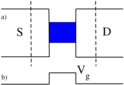
Figure 1: a) Schematic picture of the model for the QPC (dark region) between the source and drain leads, the potential at the constriction is $V_{g}$. b) Profile of the potential along the QPC.

II.1 Numerical Solution of the Unrestricted Hartree Equations

In this section we present the numerical solution of the unrestricted Hartree approximation. The charge $n_{i}$ and magnetization $m_{i}$ at each site of the central region containing the QPC are evaluated with the solution of the self-consistent equations:

$$\langle n_{i,\sigma}\rangle=-\frac{1}{\pi}\int^{\varepsilon_{F}}d\omega{Im}\left[G_{i,\sigma}^{R}(\omega)\right]$$ (5)

here the retarded Green function $G_{i,\sigma}^{R}(\omega)$ is the diagonal element of

$$G^{R}=\left[\omega+i0^{+}-H_{MF}^{0}-\Sigma^{R}(\omega+i0^{+})\right]^{-1}$$ (6)

where $H_{MF}^{0}$ is the Hartree Hamiltonian of the central part and $\Sigma^{R}(\omega+i0^{+})$ is the self energy due to the lateral regions with $m_{i}=0$.

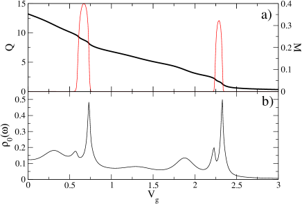
Figure 2: (a) Magnetic moment (thin line) and total charge (thick line) at the constriction of a $3$-site-wide and $9$-site-long QPC. The local interaction is $U=2.0$ and the Fermi energy is $\epsilon_{F}=-1$, with all parameters in units of $t=1$. The source and drain slabs have a width of $20$ sites. b) Local density of states at the Fermi level, averaged over the sites of the constriction, calculated in the restricted Hartree approximation.

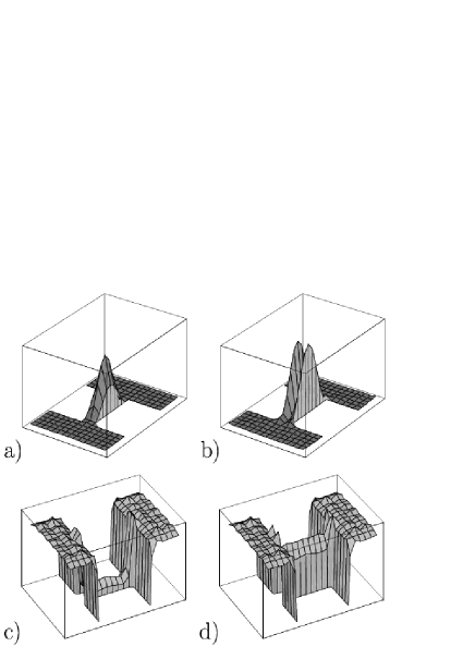
Figure 3: Spatial distribution of the a) magnetization, c) charge for $V_{g}=0.66$, and other parameters as in Fig. 2. b) and d) Same as a) and c) respectively with $V_{g}=2.27$.

We studied different QPC shapes. In the present approximation, the long range part of the electron-electron interaction renormalizes the on site energy and redefines the shape of the QPC. From hereon we take $\eta_{ij}=0$. We first present results for a model square potential shown in Fig. 1 and defined as: $\varepsilon_{i}=0$, $V_{g}$ and $\infty$ for $i$ in the source and drain, in the neck of the QPC and at the sides of it respectively. We considered a variety of QPC with $N_{0}=3$ sites in the lateral direction and $N_{1}=9$ sites in the longitudinal direction. We define the total charge and the magnetization of the contact as $Q=\sum_{i}^{{}^{\prime}}n_{i}$ and $M=\sum_{i}^{{}^{\prime}}m_{i}$ where the sum is over all the sites of the QPC. The self-consistent results are shown in Fig. 2 for a QPC of width $N_{0}$ and length $N_{1}$. For large gate voltages the total charge $Q$ in the point contact is exponentially small. As $V_{g}$ decreases $Q$ increases and for some values of the gate potential there is an abrupt increase in the total charge. The steps obtained around this point correspond to approximately one electron been transferred from the source and drain to the point contact. This behavior in $Q$ is characteristic of Coulomb blockade. Between the two first steps in $Q$ there is a spin 1/2 localized at the point contact as indicated by the magnetization curve versus $V_{g}$ shown in Fig. 2(a). The local density of states at the QPC shown in Fig. 2(b) presents a series of resonances. The resonances are associated with longitudinal modes in the QPC. The occurrence of a local magnetization at the QPC coincides with a narrow resonance crossing the Fermi energy. The first resonance has no nodes in the QPC as shown in the magnetization profile of Fig. 3(a). As $V_{g}$ decreases other resonances cross the Fermi energy and new magnetic solutions are obtained. When the first resonance of the second channel cross the Fermi energy, again a spin $1/2$ is localized in the QPC. The wave functions of the second channel have a node at the center of the QPC in the transverse direction and generate the magnetization profile shown in Fig. 3(b). For the value of $U$ considered in Fig. 2 magnetic moments are obtained only for the first resonance of each transverse channels. However, the other wider resonances may also produce local magnetic moments for larger values of $U$.

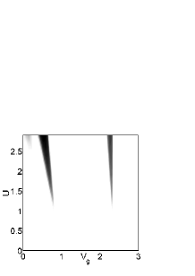
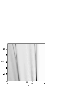
Figure 4: Phase diagram $U$–$V_{g}$ for a rectangular $3\times 9$ QPC, dark regions indicate higher values. Left: magnetization at the QPC, Right: negative derivative of the charge with respect to $V_{g}$.

In Fig. 4(a) we present the phase diagram in the parameter space [$U-$ $V_{g}$] for the $3\times 9$ QPC presented up to now. The dark regions correspond to a stable magnetic moment at the QPC. Fig. 4(b) illustrates the behavior of the charge $Q$; to analyze the behavior of $Q$ it is convenient to plot its derivative $-\partial Q/\partial V_{g}$. For small values of $U$ we obtain non-magnetic solutions for all values of $V_{g}$. However as $V_{g}$ increases and the QPC resonances cross the Fermi level, $Q$ increases and there is a maximum in $-\partial Q/\partial V_{g}$. For the parameters of the figure, magnetic solutions are obtained for $U/t\gtrsim 1$ and for values of the gate potential $V_{g}$ that make the resonances to coincide with the Fermi level. The occurrence of a magnetic solution is accompanied by a splitting of the $(-\partial Q/\partial V_{g})$ maximum, a characteristic of the Coulomb blockade regime. Fig. 5 shows the phase diagram and the behavior of $Q$ for a shorter an wider point contact. In this case larger values of U are required to produce magnetic moments. In next section we interpret these results in terms of the susceptibility evaluated in a simple approximation and make a scaling analysis to describe how the magnetic instability depends on the QPC size.

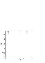
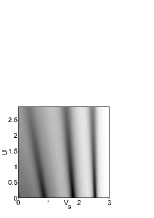
Figure 5: Phase diagram $U$–$V_{g}$ for a rectangular $5\times 6$ QPC, dark regions indicate higher values. Left: magnetization at the QPC, Right: negative derivative of the charge with respect to $V_{g}$.

The square potential optimizes resonances at the QPC and consequently favors the formation of local moments. We end this section showing some results obtained with a smoother and more realistic potential defined as:

$$V(\mathbf{r}_{i}) \equiv \varepsilon_{i}=V_{g}f(y_{i}-a_{1}/2)[1-f(y_{i}+a_{1}/2)]\times$$ (7)

$$\left\{1+10\left[f(x_{i}+a_{0}/2)+f(-x_{i}+a_{0}/2)\right]\right\},$$

where $\mathbf{r}_{i}=(x_{i},y_{i})$ is the coordinate of site $i$, $f(x)=(1+e^{x/\lambda})^{-1}$with $\lambda$ a characteristic screening length, $a_{0}$ and $a_{1}$ are the QPC width and length respectively. To describe a wedge-like point contact we take a width that varies linearly with $y_{i}$: $a_{0}(y_{i})=a_{0}+\delta a_{0}\times(y_{i}+a_{1}/2)/a_{1}$. The potential profiles for these contacts are shown in Fig. 6. In the same figure the average density of states at the point contact is also shown. For a wire-like point contact resonant states are obtained, the energies of these resonances are at the bottom of each channel. The density of states has much less structure in the case of wedge-like contacts. This shows that wire-like contacts are good candidates to develop magnetic fluctuations while wedge-like structures are not.

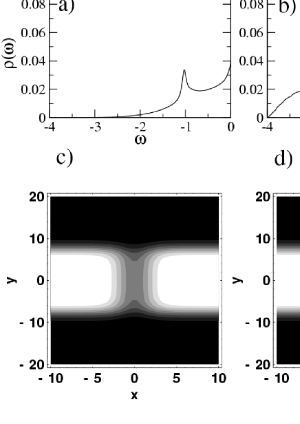
Figure 6: a) Average local density of states in the QPC, at the Fermi level for the rectangular smooth potential of c); $U=0$, $V_{g}=0.5$, $\varepsilon_{F}=-1$, $a_{0}=3$, $a_{1}=15$. b) Same as a) for the wedge shaped potential of d) and $V_{g}=1.25$, $\delta a_{0}=4.5$.

II.2 Spin Susceptibility

In the presence of an external magnetic field, the local magnetization is given by

$$m_{i}=\sum_{j}\chi_{i,j}h_{j}$$ (8)

where $h_{j}$ is the magnetic field at site $j$ and $\chi_{i,j}$ is the non-local susceptibility. In our system with no translational symmetry the non-local susceptibility depends on the two coordinates$\ \mathbf{r}_{i}$ and $\mathbf{r}_{j}$. In the Hartree approximation, the energy shift of the one particle levels is used to define an effective magnetic field given by $h_{j}=h_{ext}+Um_{j}$ where we assume a  uniform external field $h_{ext}$. The magnetization is then given by

$$m_{i}=U\sum_{j}\chi_{i,j}m_{j}+\overline{\chi}_{i}h_{ext}$$ (9)

with $\overline{\chi}_{i}=\sum_{j}\chi_{i,j}$. As we show below, $\overline{\chi}_{i}$ is just the local density of states at the Fermi energy and for $U=0$ the Pauli susceptibility depends on the coordinate as the local density of states. For $h_{ext}=0$ a non-trivial solution of equation (9) gives the onset of a spontaneous magnetization. We define the susceptibility matrix $\mathbf{\chi}$, with matrix elements $\chi_{i,j}$, and a magnetization vector $\mathbf{M}$ as a column vector with components $m_{i}$. Then equation (9) for $h_{ext}=0$ has the form of an eigenvalue problem

$$\mathbf{\chi M=}\frac{1}{U}\mathbf{M}$$ (10)

as $U\rightarrow 0$ there is no non-trivial solution of this equation. The onset of a spontaneous magnetization is given by the largest eigenvalue of $\mathbf{\chi}$ being equal to $1/U$ , the corresponding eigenvector gives the magnetic profile of the instability.

Since in the paramagnetic state the system has spin rotational invariance, we calculate the transverse susceptibility. The linear response of the system to a magnetic field along the $\mathbf{x}$ direction is:

$$\chi_{i,j}=-\ll c_{i\uparrow}^{+}c_{i\downarrow},c_{j\downarrow}^{+}c_{j\uparrow}\gg_{\omega=0}$$ (11)

where $\ll A,B\gg$ indicates the retarded Green function. In terms of the self-consistent one-particle eigenstates of the Hamiltonian $H_{HF}$ with wave functions $\varphi_{\nu}(i)$ and energies $\varepsilon_{\nu}$, the susceptibility is given by

$$\chi_{i,j}=-\sum_{\nu\mu}\varphi_{\nu}^{*}(i)\varphi_{\mu}(i)\varphi_{\mu}^{*}(j)\varphi_{\nu}(j)\frac{f(\varepsilon_{\nu})-f(\varepsilon_{\mu})}{\varepsilon_{\nu}-\varepsilon_{\mu}}$$ (12)

where $f(\varepsilon)$ is the Fermi function.

Due to the orthogonality of the one-particle wave functions, at zero temperature, we have:

$$\overline{\chi}_{i} = \sum_{j}\chi_{i,j}=-\sum_{\nu}|\varphi_{\nu}(i)|^{2}\frac{\partial f(\varepsilon_{\nu})}{\partial\varepsilon_{\nu}}$$

$$= \sum_{\nu}|\varphi_{\nu}(i)|^{2}\delta(\varepsilon_{\nu}-\varepsilon_{F})=\rho_{i}(\varepsilon_{F})$$

where we have taken the ratio between the Fermi function difference and the energy deference as the Fermi function derivative when $\varepsilon_{\nu}\rightarrow\varepsilon_{\mu}$, $\rho_{i}(\varepsilon)$ is the local density of states and $\varepsilon_{F}$ the Fermi energy. Then, inserting the above expression in equation (9), for $U=0$ we obtain $m_{i}=\rho_{i}(\varepsilon_{F})h_{ext}$.

For $U\neq 0$ in a system with no translational invariance we have to calculate the non-local susceptibility, a matrix of dimension equal to the number of sites of the sample. To simplify the problem we assume that $U$ is much smaller than the Stoner value that generates a global instability, consequently a non trivial solution of equation (10) should have the magnetization concentrated in the region of the point contact. We assume that far from the contact $m_{i}=0$ and look for solutions with $m_{i}\neq 0$ only if $i$ belongs to a small region $\ R$ that includes the contact. Then we have to calculate a reduced matrix susceptibility $\chi_{i,j}$ with $i,j$ in $R$.

Since even in the paramagnetic state, and due to the charge redistribution close to the point contact, the one-particle states of $H_{HF}$ depend on $U$ in a non-trivial way, the largest eigenvalue $\kappa$ of the susceptibility depends on $U$ and the instability condition is a self-consistent equation:

$$\kappa(U)=1/U$$

and its solutions have to be obtained numerically.

II.3 The Resonant State Approximation

Here we present some analytical results based on the fact that, for high gate voltages, the local density of states at the point contact present well defined resonances. By varying the gate voltage the position of the resonances can be tuned to coincide with the Fermi level. When this occurs, for small quantum point contacts where the quantization effects are important, the transport and magnetic properties of the contact are dominated by a single resonant state and in what follows we consider this situation. This is a valid approximation as long as the width of the resonance remains much smaller that the separation between resonances. The non-local susceptibility is now given by

$$\chi_{i,j}=-\widetilde{\sum_{\nu\mu}}\varphi_{\nu}^{*}(i)\varphi_{\mu}(i)\varphi_{\mu}^{*}(j)\varphi_{\nu}(j)\frac{f(\varepsilon_{\nu})-f(\varepsilon_{\mu})}{\varepsilon_{\nu}-\varepsilon_{\mu}}$$ (14)

here the decorated sum indicates summation over all states belonging to a single resonance. For $i$ in the point contact, the corresponding wavefunctions can be written as

$$|\varphi_{\nu}(i)|^{2}=|\alpha_{m}(i)|^{2}\frac{\gamma/\pi\rho_{\nu}}{(\varepsilon_{\nu}-\Delta)^{2}+\gamma^{2}}$$ (15)

where $\alpha_{m}(i)$ is the wave function of the QPC, $\gamma$ and $\Delta$ are the width and the energy of the resonant state $m$ and $\rho_{\nu}$ is the density of states. Since we can work with real wavefunctions, they can be taken as the square root of the above expression and the susceptibility can be put as

$$\chi_{i,j}=|\alpha_{m}(i)|^{2}|\alpha_{m}(j)|^{2}\chi_{res}$$ (16)

with the susceptibility of a resonant state given by

$$\chi_{res} = -\int d\varepsilon_{\nu}d\varepsilon_{\mu}\frac{(\gamma/\pi)^{2}}{[(\varepsilon_{\nu}-\Delta)^{2}+\gamma^{2}][(\varepsilon_{\mu}-\Delta)^{2}+\gamma^{2}]}\times$$ (17)

$$\frac{f(\varepsilon_{\nu})-f(\varepsilon_{\mu})}{(\varepsilon_{\nu}-\varepsilon_{\mu})}$$

The susceptibility matrix has the form $\mathbf{\chi}=\chi_{res}\mathbf{A}$ where the matrix $\mathbf{A}$ can be put as

$$\mathbf{A=}\left[\begin{array}[]{c}|\alpha_{m}(1)|^{2}\\ |\alpha_{m}(2)|^{2}\\ :\\ |\alpha_{m}(N)|^{2}\end{array}\right]\left[|\alpha_{m}(1)|^{2},|\alpha_{m}(2)|^{2}..|\alpha_{m}(N)|^{2}\right]$$ (18)

and the instability condition becomes

$$\alpha U\chi_{res}=1$$ (19)

where $\alpha$ is the largest eigenvalue of the matrix $\mathbf{A}$. From the form of $\mathbf{A}$ it is clear that the vector

$$\mathbf{M}=\left[\begin{array}[]{c}|\alpha_{m}(1)|^{2}\\ |\alpha_{m}(2)|^{2}\\ :\\ |\alpha_{m}(N)|^{2}\end{array}\right]$$ (20)

is an eigenvector with eigenvalue $\alpha=\sum_{i}|\alpha_{m}(i)|^{4}$ and that all other eigenvalues are zero. The condition for the formation of a magnetic moment at the point contact is

$$U_{eff}\chi_{res}=1$$ (21)

where $U_{eff}=\sum_{i}|\alpha_{m}(i)|^{4}U$ is the effective Coulomb repulsion for two electrons at the QPC state $m$ with spacial wavefunction $\alpha_{m}(i)$. If the resonance is centered at the Fermi level, this condition is simply

$$U_{eff}=\pi\gamma/2$$ (22)

For small $U$ and an arbitrary potential form of the point contact defined by the potential $V(\mathbf{r}_{i})$, the Hartree solution can be used to estimate $\alpha_{m}(i)$ and $\gamma$.

Now we compare this criterion with the full unrestricted Hartree calculation for the lowest energy resonance. For the square potential of Fig. 1 the $U=0$ eigenfunctions $\alpha_{0}(i)$ are:

$$\alpha_{0}(i) = \sqrt{\frac{2}{(N_{0}+1)}}\sin(\frac{\pi}{a(N_{0}+1)}x_{i})\times$$ (23)

$$\sqrt{\frac{2}{(N_{1}+1)}}\sin(\frac{\pi}{a(N_{1}+1)}y_{i})$$

here $a$ is the lattice parameter, $aN_{0}$ and $aN_{1}$ are the QPC width and length respectively. As this wavefunction is hybridized with the right and left reservoirs it acquires a width $\gamma=2\pi\rho V_{eff}^{2}$ where $\rho$ is the density of states of the reservoir and the effective hybridization is

$$V_{eff}\simeq t\sum_{i\in edge}|\alpha_{0}(i)|$$ (24)

the sum is over all the sites of the QPC that are at one edge (right or left), hybridized with the reservoir. With this estimation and the condition of equation (22) we obtain the critical value $U_{c}^{*}$ of the Coulomb repulsion for the occurrence of a magnetic solution shown in table 1. The comparison with the values obtained using the fully unrestricted Hartree approximation is very good in particular for long and narrow point contacts.

Table 1: Critical values of $U$ for the appearance of magnetic solutions.

$N_{0}\times N_{1}$	$U_{c}/t$	$U_{c}^{*}/t$
$3\times 11$	$0.55$	$0.57$
$3\times 9$	$0.85$	$0.84$
$4\times 7$	$1.50$	$1.76$
$5\times 6$	$2.25$	$2.49$
$5\times 5$	$3.18$	$3.96$

For the second longitudinal resonance of the first channel in the case of the $3\times 9$ geometry, we find the same $U_{eff}$ as for the first resonance while the width of the resonance becomes $\gamma^{\prime}\sim 3.6\gamma$ [as observed in Fig. 2(b)], therefore giving $U_{c}^{\prime}/t\sim 3.1$ in good agreement with the corresponding phase diagram shown in Fig. 4.

Finally we can make a approximate scaling analysis for large systems: the effective repulsion in a single resonance $U_{eff}=\sum_{i}|\alpha_{m}(i)|^{4}U\sim U/(N_{0}\times N_{1})$ and the effective width of the resonance is proportional to the square of the hybridization of equation (24), $\gamma$ $\sim$ $\rho t^{2}/N_{1}^{3}$. These estimations lead to a critical value of $U$ that at resonance scales with the size of the point contact as $U_{c}$ $\sim$ $\rho t^{2}N_{0}/N_{1}^{2}$. Numerical estimations of the mean field critical value for large systems are in agreement with this scaling.

III Conclusions

We have presented results for the formation of local magnetic moments in point contacts. We used a Hubbard-like model to describe point contacts formed in a two dimensional system. The contact is defined in terms of a potential $V(\mathbf{r})$ that can be varied with a single parameter $V_{g}$ representing a gate voltage. We calculate the magnetic moment using the unrestricted Hartree approximation. For a square potential, the system shows a marked tendency to form a localized moment at the point contact each time a new channel is tuned to the Fermi energy. In this conditions the critical value of the local repulsion $U$ is almost an order of magnitude smaller than the Stoner critical value for an homogeneous system. For the parameters of figure 4 the critical value for the first resonances is $U\sim t$. Using the effective mass and electron density characteristic of GaAs-AlGaAs hetherostructures, we can take a lattice parameter $a=10nm$. With these numbers, the results of the figure correspond to a point contact of $30nm\times 90nm$ and the critical value of $U$ gives an effective interaction $U_{eff}\sim 0.5meV$.

In long contacts defined with a square potential, the second longitudinal resonance may also generate a local moment for moderate values of $U$. This is a consequence of the square potential that optimizes resonances each time the Fermi wavelength is commensurate with the contact length. For more realistic potentials only the first longitudinal resonance of each channel may generate a local moment. Moreover, for wedge-like contacts we found no evidence of moment formation in the Hubbard type models. The numerical results are interpreted in terms of a simple one-resonance approximation. We also present a simple a scaling argument to interpret the general dependence of the magnetic instability with the point contact dimensions.

We end by stressing that the Hartree calculation, that breaks the spin symmetry, only gives a criterion that allows to identify the region of parameter space were the low temperature physics may be dominated by magnetic fluctuations. In this particular regions a Kondo-like model may be used to describe the spin fluctuations Cornaglia and Balseiro (2004); Meir et al. (2002).